SOFT BUDGET CONSTRAINTS IN A DYNAMIC GENERAL
EQUILIBRIUM MODEL
Enrique Gilles
SERIE DOCUMENTOS DE TRABAJO
No. 81 Marzo 2010
Soft budget constraints
in a dynamic general equilibrium model
Enrique Gilles
∗Abstract
This paper considers an overlapping generations model in which capital investment is financed in a credit market with adverse selection. Lenders’ inability to commit ex-ante not to bailout ex-post, together with a wealthy position of entrepreneurs gives rise to the soft budget constraint syndrome, i.e. the absence of liquidation of poor performing firms on a regular basis. This problem arises endogenously as a result of the interaction between the economic behavior of agents, without relying on political economy ex-planations. We found the problem more binding along the business cycle, providing an explanation to creditors leniency during booms in some Latin-American countries in the late seventies and early nineties.
JEL Codes: E22, E44, D21, D82.
∗This paper benefited from useful comments by Martial Dupaigne, Patrick F`eve, J´erˆome
Glachant, Fernando Jaramillo, Jorge Ponce, Franck Portier, St´ephane Straub, M´onica Vargas, and seminar participants at LACEA 2005 and Universidad de Los Andes 2007. All remaining er-rors are my own. Universidad del Rosario, Bogot´a, Colombia. [email protected].
The findings, recommendations, interpretations and conclusions expressed in this paper are those of the author and not necessarily reflect the view of the Department of Economics at Universidad del Rosario.
1
Introduction
In this paper we propose a dynamic general equilibrium model of an economy suffering from the soft budget constraint (SBC) syndrome. This phenomenon, initially analyzed by Kornai (1986) in the study of transition economies, is charac-terized by the survival of inefficient firms thanks to the financial support of other institution. The softening of budget constraints, however, may occur without any external support but as the result of asymmetric information in a borrower-lender relationship. Indeed, it may be the case that refinancing bad projects is in the lender’s best business interest. Such a situation may arise whenever a lender has initially funded a project which type was not known at the contracting stage. When some information about the quality of the project is revealed, and given the sunk nature of the initial funding, lenders may want to extend extra funding to allow the project to be finished, so as to minimize losses.
This second rationale for softness is the one chosen in this paper. Of course, we do not rule out there are political factors implying that inefficient firms are al-lowed to survive (Kornai’s original explanation), but we consider economic factors are, in some contexts, enough to show the existence of the syndrome.
Indeed, there has been evidence of it in some Latin American countries. It is the case of Uruguay and Argentina during the late seventies, in the context of financial liberalization processes and the international bonanza in capital mar-kets. In that period, bank lending has gone through a great expansion and there is evidence that project screening and monitoring were at best reduced. The ini-tial funding as well as the refinancing of non-performing projects were therefore highly likely. To give a very illustrative example of the aggressive behavior of banks in giving loans, the popular saying during the credit boom in Uruguay was: “You could never get less than twice the money you asked for”.1
Therefore, we can think of refinancing of bad projects as a by-product of lending booms. In fact, this has been mentioned in the literature of lending booms, for example in Gourinchas et al (2001). They characterize the pattern of
a typical lending boom in Latin America and the rest of the world, identifying three main ingredients: financial liberalization, large capital inflows and a failed program of stabilization based on the exchange rate. The causes of lending booms are a combination of imperfections in the financial architecture and misaligned incentives at the microeconomic level (e.g. a poor regulation of the financial sector, a dampened monitoring activity, the expectation of a future bailout from the government) that implies riskier projects are undertaken. Finally, they show these episodes are accompanied by an investment boom.
This paper analyzes the effects of refinancing of bad projects in a general equilibrium model. The setting is a neoclassical growth model with overlapping generations, where physical capital is financed through a credit market with ad-verse selection.
Our results point out that refinancing of inefficient projects (soft budget con-straint) happens, and that it is more likely during expansions. In other words, periods of bonanza are characterized by more indulgent credit market conditions that are translated into more refinancing. In particular, entrepreneurial wealth plays a key role in this result, since it is the link between the performance of the economy as a whole and the investment decisions entrepreneurs take. That is, borrowers net worth during expansions is high and this facilitates lending.
For the general equilibrium setting we draw on Bernanke and Gertler (1989), who consider the effects of a costly state verification setting in the credit mar-ket on capital investment and on business cycles. We also follow Azariadis and Chakraborty (1999) who, in a similar model, incorporate a richer specification of verification costs. In this sense, our model continues this tradition that analyzes the relationship between borrowers’ net worth and macroeconomic activity.
Among the literature on soft budget constraints applied to credit markets there is a set of papers that follows the Dewatripont-Maskin (1995) (DM) model. The basic setting includes entrepreneurs endowed with good and poor projects, which are respectively efficient and inefficient, and lenders who provide the initial investment. Given adverse selection, lenders may initially fund and even refinance inefficient projects. There is no government, the decision to refinance is linked
to the existence of sunk costs, which implies a redefinition of the profitability criterium. Ex-ante, lenders do not want to fund inefficient projects, hence they are willing to deter poor projects to be submitted through a threat of termination. However, in the event that lenders have initially funded such projects, that threat could well not be credible. Ex-post, that is after default occurred, and given that initial funding is considered as sunk, it can be the case that bringing poor projects to completion (by injecting new funds) is in everybody’s best business interest. Lenders would recover some of the incurred losses, while entrepreneurs usually have enough incentives to see their projects finished rather than liquidated. Being aware of these mechanisms at the contracting stage, entrepreneurs endowed with poor projects may be tempted to submit them.
In such a context of agents rationality and profit maximizing behavior, one of the puzzles is to find out why soft budget constraints are not so prevalent in market economies. In Dewatripont and Roland (1999) an answer is advanced stating that hardening soft budget constraints is a matter of institutional design. In this DM tradition, we find models of soft budget constraint applied to dif-ferent settings, but mainly focused in credit markets. Bergl¨of and Roland (1997) point out that refinancing poor projects may crowd out investment when the average quality of new projects is low enough, hence giving an explanation to the coexistence of soft budget constraints and credit crunches. Bergara, Ponce and Zipitr´ıa (2003) propose a unified framework to study both political an economic-induced softening. Mitchell (2000) proposes a new taxonomy of models based on ex-ante and ex-post efficiency criteria that allows to identify two classes of mod-els. Indeed, not all SBC configurations incorporate ex-post efficiency as in DM, but it can also be the case of ex-post inefficiency. She then provides an example of the latter, in the context of banking crises, through a model of the SBC where creditor passivity –under the form of debt rolling over– has the leading role on explaining the softening.
Therefore, the effects of the syndrome have been studied in a diversity of environments, to which we should add fiscal federalism, decentralization and political economy. What the above mentioned articles have all in common is
their microeconomic approach. This paper is, to the best of our knowledge, the first attempt to incorporate the soft budget constraint syndrome into a dynamic general equilibrium setting.
This paper is organized as follows: in section 2 we present the general equi-librium setting with a description of agents, technologies, preferences and envi-ronment. Section 2.2 explains the credit market characteristics, and presents the full information and imperfect information cases. Section 3 analyzes the effects of the syndrome in the general equilibrium setting: formation of physical capital, identification of winners and losers, and dynamic properties of the model. Section 3.3 tests the empirical predictions of the model. Finally, Section 4 concludes.
2
The model
Consider an overlapping generations (OLG) model with constant population in which each generation lives two periods. Each individual receives a labor income when young, and saves in order to consume when old. There are no bequests. Time is infinite in the forward direction, divided into discrete periods indexed by t. In what follows we complete the description of this economy.
2.1
Setting
Agents. There is a countable infinity of individuals who are divided into two classes of agents: an exogenous fractionηis endowed with an investment technol-ogy through which physical capital is built. These agents are called entrepreneurs. The remaining fraction 1−η are households, which we call lenders since they are credit suppliers. Among entrepreneurs we will distinguish between good and poor ones, as will be defined later. All agents are risk-neutral.
Endowments. Every individual (entrepreneur or lender) has a fixed labor en-dowment to be used in his first period of life. This enen-dowment is constant across time, Lt=L.
markets: There are two storage technologies in this economy, which allow to have funds when old. The storage technology for lenders yields the gross payoffR >1, while the one for entrepreneurs yields only ˆR <1.
Preferences. Individuals, either entrepreneurs or lenders, have preferences over consumption when young and old, represented by the following utility function:
U(ct) +ρEt(dt+1), (1)
where ct is the agent’s consumption when young and dt+1 is her consumption
when old. U is concave and ρ is a discount factor. Note that individuals are risk-neutral with respect to second period consumption, this assumption allows us to avoid risk-sharing considerations. Agents’ consumption and savings will depend then on the relevant interest rate as well as on the wage rate. Calling c∗
t(R) the optimal consumption of individuals when young, savings are given by:
st =wtL−c∗t(R). (2)
We will work under the simplifying assumption that total lenders’ savings in this economy are high enough so as to fund all projects. In terms of the model, we suppose that the proportion (1−η) of lenders is large enough, and this implies that there is always a positive level of storage and the marginal rate of return for lenders is R.
Goods and technologies. There are two goods in this economy: an output (or consumption) good and a capital good. The output good is produced using a constant returns to scale technology that uses both the capital good and labor as inputs. We write the production function in per capita terms:
yt= ˜tf(kt), (3)
where f is concave, kt is per capita physical capital (assumed to be fully
depre-ciated in one period), and ˜t is a random aggregate productivity shock, which is
i.i.d. over time and continuously distributed over a finite positive support, with mean .
The output good produced in period t can be used during the same period either to consume, to lend to entrepreneurs, or to store using the storage tech-nologies.
The physical capital good is produced by entrepreneurs, who own the technol-ogy that come into the form of “investment projects”. Each entrepreneur has one investment project, which lasts one period, needs one unit of the output good as initial investment, and can be either good or poor: while the former yield positive net present values, the latter do not2. We identify a good entrepreneur
as an entrepreneur who owns a good project, and the same applies for poor en-trepreneurs.
Assumptions. This economy can be characterized by some features which best fit to a developing country, in particular in what concerns to imperfect capital markets. We next present and discuss these assumptions.
First, we work with the assumption that there are rigidities in the credit mar-ket that translate into the existence of different storage technologies for lenders and entrepreneurs. It is well known that such imperfections are common in many third world economies, in which some agents have access to international compet-itive markets, while others have only access to native capital markets. The latter are characterized by the presence of non-competitive practices, credit constraints, administrated interest rates, lack of arbitrage, among other imperfections. This will allow us to limit the space of possibilities of lenders and entrepreneurs.
Second, lenders are disperse and thus passive, they do not have any screening or monitoring device that would allow them to better discriminate between good and poor projects.
Third, let us introduce the assumption that entrepreneurial saving, despite being known at the contracting stage, is not available at that time but only at an interim stage. We can suppose entrepreneurs have to compulsorily deposit their savings into the storage technology. This is a straightforward way to make entrepreneurs ask for credit to finance their projects. Moreover, lenders have to
2By using the term poor instead of, for example,Bad, we are simply adopting the terminology
entirely finance the initial investment of projects.
Finally and for simplicity, we rule out any possibility that entrepreneurial saving may be contracted upon. Again, these last two assumptions are adequate in the context of underdeveloped economies, characterized by poor institutional frameworks and inefficient judiciary procedures. In sum, these assumptions serve the purpose of facilitating the analysis and at the same time they adjust our setting to the Dewatripont-Maskin basic framework.
t
period t period t+ 1
shock ˜t realized
young agents are born production, income
consumption, storing borrowing-lending
old agents consume and die.
projects’ types
and abilities revealed refinancing decisions kt+1 determined shock ˜t+1 realized periodt+ 1 agents are born production, income period t agents
consume and die ...
Figure 1: The life of agents
Figure 1 illustrates the life span of agents, the main features of the general equilibrium setting, together with the decisions agents take at each time. At any period t a new generation of lenders and entrepreneurs are born, who coexist with period-(t−1) born agents (old agents in periodt). Production is done with the labor endowment of generation t together with the capital built in period (t−1), and the realized value of the productivity shock ˜t, as equation (3)
estab-lishes. Young agents receive their labor income and old agents their capital factor remuneration and the returns from storage. Period-t lenders consume, lend to entrepreneurs and store. Entrepreneurs consume, store, and borrow from lenders. At the end of periodt, next period physical capitalkt+1 is determined. When this
generation arrives to old, in (t+ 1), new production is realized and these agents receive their capital returns which, added to the returns from storage determines their consumption when old.
2.2
Credit Market
We now describe the credit market, in which entrepreneurs and lenders meet to fund projects. In doing so we are in a partial equilibrium framework, this means the level of entrepreneurial savings sE
t, the productivity shock ˜t, the wage rate
wt, the expected relative price of capital ˆqt+1 are all taken as given.
The key feature of this borrower-lender relationship is given by the presence of asymmetries of information between both types of agents. We assume that at the contracting stage lenders are not able to distinguish between a good and a poor project, which is then the entrepreneur’s private information. Lenders face a pool of applicants for funding. However, they do know that a given project has a probability α of being good and (1−α) of being poor.
Both good and poor projects need an initial investment of one unit of the output good. Since the level of entrepreneurial savings –despite being known– is not available at the contracting stage, this initial investment is entirely provided by lenders. A given project –if completed– yields with certaintyκunits of physical capital at the end of the period, to be sold at relative price qt+1 in the next one.
The gross expected payoff of a completed project is then ˆqt+1κ.
The poor project technology is only distinguished from the good one by the fact that, at an interim stage, an extra injection of funds is required in order to bring the project to completion. It is otherwise impossible to continue it, and the liquidation value is given by a fixed amountRLwhich is entirely seized by lenders.
In case the project is refinanced, it yields the gross expected payoff ˆqt+1κ, just
as the good project. At the interim stage, we can distinguish between good and poor projects, since poor entrepreneurs need extra funding in order to complete their projects and thus they will ask lenders for refinancing.
at the end of the period, yielding the following expected net present value3:
NP VG = ˆqt+1κ−R. (4)
Assumption 1 NP VG >0.
We will insure below that this assumption holds. The fact that the relevant price is ˆqt+1 also simplifies the analysis, since all the decisions taken in t depend only
on expectations about the next-period productivity shock (i.e. on , which we assume fixed), rather than on its actual value (i.e. on ˜t+1).
Poor projects. The amount of extra funds needed by poor projects will in turn depend on poor entrepreneurs’ own characteristics: we assume that the class of poor entrepreneurs is itself not homogeneous. This heterogeneity comes from the fact that each poor entrepreneur has an idiosyncratic characteristic that reflects his ability to complete the project. At the contracting stage, a representative entrepreneur of this class knows he has a poor project, but he does not know how well he will perform in taking the project to completion. He needs to invest himself into the project, learn by doing, in order to know more and find out his level of ability. Hence, we assume that abilities are unknown at the contracting stage, and that this is particularly true for poor entrepreneurs themselves. At the interim stage, this process of information acquisition is completed and abilities become publicly observed4.
Then, different abilities will be translated into different needs of funds at the interim stage, in a way that a highly skilled entrepreneur needs less funds to complete the project. We have thus an opposite correspondence between these two variables. poor entrepreneurs are indexed by i, and ability (extra funding) is represented by the parameter θi. Let us assume that it is uniformly distributed
in the interval [θ
¯,θ¯] among poor entrepreneurs, with ¯θ−¯θ = 1.
3We should interpret “present” as corresponding to values at periodt+ 1.
4Another interpretation for this feature would be an exogenous liquidity shock affecting poor
Assumption 2 NP VPi <0 ∀θi5.
The expected net present value of agent i’s poor project is
NP VPi = ˆqt+1κ−R(1 +θi) (5)
It is then ex-ante inefficient to refinance a poor project, and it follows that an entrepreneur with a low value ofθ is “less inefficient” in the continuation activity. However, under some circumstances it may be the case that lenders are willing to refinance poor projects at the interim stage. Such a situation describes a soft budget constraint episode, in which there is a discrepancy between the ex-ante and ex-post criteria: despite the project is poor and thus it should be liquidated, it may occur that it could be efficient ex-post, i.e. once default occurred and the initial investment is considered as sunk. In such a case, in their quest to recover some of the initial sunk investment, lenders will only pay attention to the continuation and liquidation payoffs, the latter given by a fixed amount RL <1.
Assumption 3 qˆt+1κ−Rθ
¯ < RL.
This assumption tells us that –absent any entrepreneurial contribution– it is optimal for lenders to liquidate poor projects, since in such a case the liquidation payoff is higher than the continuation payoff6. The refinancing decision will be
then based on an entrepreneur’s contribution: the entrepreneur is called to put up a part of his savings (˜sE
t ) in order to be refinanced.
Assumption 4 The verifiable payoff is a fraction γ of the total gross payoff.
We are assuming that entrepreneurs, given their direct involvement in the project’s management, are able to deviate to their pockets a fixed proportion (1−γ) of the projects gross payoff.
5The expected value of the random shock is set to = 1. Then we assume R
κf0(κη) <1 <
(1+θ
¯)R
κf0(ακη), which is sufficient to guarantee the existence of both Good and Poor projects. This
is valid for some reasonable parameter configurations.
6To guarantee Assumption 3 holds, and given the assumptions on it is sufficient to add
the assumptionR < RL
1−αθ
¯
t= 0
Contract signed Initial investment=1
t= 1/2
Abilities (extra funding)θi
Refinancing decisions t= 1 Outcome ˆ qt+1κ ˆ qt+1κ RL (1−σ) Refinancing α Good Projects (1−α) Poor Projects σ Liquidation
Figure 2: Credit market timing
In sum, the timing is presented in Figure 2. At the contracting stage, lenders and entrepreneurs meet to fund projects. The level of current entrepreneurial savings is publicly observed but it is not yet available, so it cannot be used to be invested into projects and thus lenders provide the entire initial investment. En-trepreneurs’ abilities are unknown for every agent –including poor entrepreneurs themselves– but their distribution is common knowledge. Both lenders and en-trepreneurs take the decisions of respectively fund any project, and submit their projects for funding. At the interim stage, poor projects can be distinguished from good ones, and each poor entrepreneur is characterized by his level of abil-ity. Lenders ask for an entrepreneurial contribution in order to refinance such projects, otherwise there is liquidation for a fractionσ, to be defined below. Abil-ities, together with the level of entrepreneurial savings, may determine that some poor entrepreneurs will be able to get refinancing.
2.2.1 The perfect information case
Let us first introduce the perfect information case. For ease of notation and given that we are in partial equilibrium, we refer to the gross payoff of a terminated project asRS = ˆqt+1κ, we use the subscript S for successful projects (either good
projects or poor projects that are refinanced). If the project is liquidated, we keep RL. We also use superscripts to denote the agent (lenders: L, entrepreneurs: E).
When lenders can observe the type of projects entrepreneurs have, they will only fund good projects. Lenders’ expected payoff writes:
ΠLS =γRS−R >0. (6)
Entrepreneurs get the remaining share (1−γ).
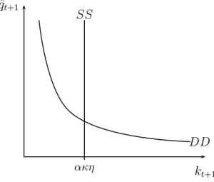
The supply of physical capital is given by the following curve, that we call hereafter the SS curve:
kt+1 =ακη. (SS)
The next-period stock of (per capita) capital kt+1 is fixed, and is given by the
units of physical capital a good project can create (κ), multiplied by the total number of such projects in the population, αη. On the other side, the demand curve DD is given by the equality between the expected price of capital and its expected marginal productivity.
ˆ
qt+1 =f0(kt+1). (DD)
This curve is downward sloping since f is concave, and recall that is the mean of the productivity shock. In each period t, ˆqt+1 and kt+1 are determined as the
intersection of the supply and demand curves of capital, as Figure 3 shows. The dynamics in the full information case are simple: since no period-t vari-able is involved in SS and DD, both the expected price and the quantity of physical capital will be constant over time. Investment is then fixed, and re-minding that labor supply so is, the only origin of fluctuations comes from the aggregate productivity shock ˜t. With full information, all good projects are
already financed, therefore any extra funds will serve to increase storage and consumption.
ˆ qt+1 kt+1 ακη SS DD
Figure 3: Equilibrium in the perfect information case
2.2.2 The asymmetric information case
When entrepreneurs types are not observable, lenders decide at the contracting stage whether to fund any project they face, and entrepreneurs decide whether to submit their projects for funding. At the interim stage, when all the information becomes publicly observed, lenders decide on extending extra funding to poor projects, while poor entrepreneurs themselves decide on continuing or not.
Lenders’ financing and refinancing decisions. Lenders financing decisions depend on the mix of good and poor projects existing in the economy as well as on the refinancing conditions that will appear at the interim stage. For a particular lender to finance any project, the net expected payoff from funding projects must be at least equal to zero,
ΠL =αΠL G+ (1−α) σΠL liq+ (1−σ)ΠLref ≥0 (7)
The total net expected payoff are composed by the net expected payoff from funding a good project (with probability α) and the net expected payoff from funding a poor project (with probability (1−α)). Among them, some will be liquidated, with probabilityσ(to be defined below). The remaining poor projects
will be able to be refinanced.
The expected payoff from funding a good project is given by
ΠLG=γRS −R >0. (8)
For poor projects, we need to analyze what happens at the interim stage, when lenders observe the type of entrepreneur they have funded. Recall that it is at this time possible to distinguish within poor entrepreneurs according to their level of ability. Therefore, lenders have to take a decision concerning refinancing or liquidating them. At a first sight, taking into account that a poor project is –by definition– a negative expected present valued one, liquidation would seem like the best strategy for lenders. However, given the sunk nature of the initial investment, it could be the case for refinancing. In order for continuation to occur, and taking into account there is no possibility of refinancing without an entrepreneurial contribution, the entrepreneur should contribute with an amount ˜
sE
t of her savings, borrowing the remaining amount θi − ˜sEt from the lender.
Entrepreneurs may then make the lender’s refinancing payoff greater than the liquidation payoff, forcing the project’s continuation whenever
γRS−R(θi−s˜Et)≥RL. (9)
From the point of view of lenders, an entrepreneurial contribution that makes this inequality binding would be enough to extend refinancing7. Let us then define,
for a given level of entrepreneurial savings sE
t the threshold θs as the marginal
poor entrepreneur, that is, the one who leaves the lender indifferent between continuation and liquidation (equation (9) is binding),
θs(sEt ) = γRS−RL
R +s
E
t . (10)
It follows that any poor entrepreneur with level of abilityθi ≤θshas enough assets
so as to be refinanced. Let us call them high-ability entrepreneurs, whereas the contrary applies for θi > θs, which we call low-ability entrepreneurs.
7We assume that, if indifferent between continuation or liquidation, lenders decide to go
With the above facts, define σ(sE
t ) as the fraction of poor entrepreneurs that
will be liquidated σ(sEt ) = Z θ¯ θs(sE t ) f(θ)d(θ) = ¯θ−θs(sEt ), (11)
and the fraction (1−σ) of poor entrepreneurs that will be refinanced, 1−σ(sEt) =
Z θs(sEt)
θ
¯
f(θ)d(θ) = θs(sEt )−¯θ. (12)
Note that a higher value of entrepreneurial savings means a higher fraction of poor projects that get refinancing.
Given that lenders are passive, the necessary amount ˜sE
t that an entrepreneur
θi ≤θs must contribute with in order to be refinanced is given by
˜
sEt (θi) =θi −
γRS−RL
R , (13)
which follows from equation (9). On the other hand, lenders will cover the re-maining
θi−s˜Et (θi) =
γRS−RL
R . (14)
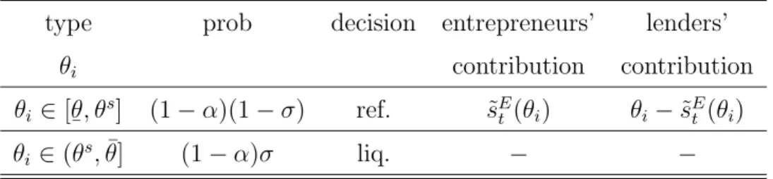
Table 1 summarizes the findings of this subsection8. There is then poor projects’
Table 1: Decisions at interim stage
type prob decision entrepreneurs’ lenders’
θi contribution contribution θi ∈[θ ¯, θ s] (1−α)(1−σ) ref. s˜E t (θi) θi−s˜Et (θi) θi ∈(θs,θ¯] (1−α)σ liq. − −
continuation (i.e. soft budget constraint) for the first group of poor entrepreneurs, and liquidation for the other one. In case of refinancing, lenders’ interim con-tribution is fixed, whereas entrepreneurs’ concon-tribution is increasing in types. In
8For ease of notation, we omit hereafter the dependence ofσon entrepreneurial savingssE t.
the second group, –high levels of θ– there is liquidation, so no contributions are involved.
The expected payoff of lenders who financed a low-ability entrepreneur, θi ∈
(θs,θ¯] is given by ΠL liq =RL−R <0, and for θi ∈[θ ¯, θ s] ΠL ref =γRS−R h 1 + ˆθ−s˜E t (ˆθ) i <0,
where ˆθdenotes the expected value ofθconditional onθi belonging to the relevant
range for high-ability entrepreneurs. Note that, substituting the expression for ˆ
θ−s˜E
t (ˆθ) –see equation (14)–, we can rewrite this equation as
ΠL ref =γRS−R 1 + γRS −RL R =RL−R < 0. (15)
This is the same expected payoff that a lender would get by terminating the project, since entrepreneurs need to contribute up to the point in which lenders are just indifferent between continuation and liquidation. With these ingredients, we can rewrite lenders participation constraint at the contracting stage , equation (7), as
ΠL =α(γRS−R) + (1−α)(RL−R)≥0. (16)
Equation (16) then governs lenders decision to fund projects at the contracting stage. This decision depends on the mix of good and poor projects in the en-trepreneurs population given by the exogenous parameterα, as well as the payoffs RS and RL.
Entrepreneurs’ investment decisions. The decision that an entrepreneur has to take at the contracting stage is whether to submit her project for funding. Given our setting it is straightforward to see that a good entrepreneur will always submit her project: by doing so she gets a proportion (1−γ) of the gross payoff without contributing to funding. Formally, she will submit it as long as
For a poor entrepreneur, the decision to submit her project at the contracting stage will depend on the probability of being refinanced at the interim stage, and in such a case on the opportunity costs of the funds she will have to put. Recall that entrepreneurs have a primitive storage technology available, and that at the contracting stage they do not know their levels of ability, which is only revealed at the interim stage.
The poor entrepreneur expected payoff if she submits her project is com-posed by two terms: First, if she turns out to be a low-ability entrepreneur, with probability σ(sE
t ), her project will be liquidated so her payoff will be zero.
And second, in the case she is a high-ability entrepreneur, which occurs with probability 1−σ(sE
t )
, she will be allowed to continue provided she contributes at interim with an amount ˜sE
t(θi). Then, the poor entrepreneur’s participation
constraint at the contracting stage is given by (1−σ)h(1−γ)RS−Rˆs˜Et (ˆθ)
i
>0. (18)
This individual rationality constraint tells us that, in order that a poor en-trepreneur submit her project when young, the expected payoff from it must be greater than zero. Notice that if the liquidation probability is equal to one, these entrepreneurs are not willing to submit their projects. They know ex-ante that they will be liquidated for sure. This equation illustrates expectations of a future bailout, their decision will depend on the current level of entrepreneurial savings, sE
t .
At the interim stage, we saw lenders may extend refinancing to those poor entrepreneurs called high-ability ones. Once entrepreneurs’ abilities become ob-served, these entrepreneurs will be willing to be refinanced if the gross expected payoff from the project exceeds their opportunity cost of funds, i.e. if
(1−γ)RS ≥Rˆ˜sEt (θi), for θi ≤θs(sEt )
In order that every high-ability poor entrepreneur may be willing to continue, it must be the case that
since the maximum value of ˜se
t(θi) is sEt , when θi =θs(sEt ).
Equilibrium in the credit market
Proposition 1 Soft budget constraint equilibrium. If
i. α≥ R−RL γRS−RL ≡α ii. (1−γ)RS ≥0 iii. (1−σ)h(1−γ)RS−Rˆs˜Et (ˆθ) i >0 iv. γRS−R(θi−s˜Et)≥RL. v. (1−γ)RS ≥Rsˆ Et .
there exists an equilibrium with soft budget constraint.
Proof. The first equation is lenders’ participation constraint at the contracting stage, equation (16), it states that in order to finance any project, the propor-tion of good projects must be higher than a threshold α. The second and third equations are the entrepreneurs participation constraints at the contracting stage. The fourth equation is the continuation rule for poor projects, which acts as a participation constraint for lenders at the interim stage. Finally, the last equation is the participation constraint of poor entrepreneurs at interim. If all of these conditions hold, we have an equilibrium in which all project are initially funded and some poor projects end up refinanced, i.e. the equilibrium entails soft budget constraint. 2
In the soft budget constraint equilibrium, lenders refinance a fraction 1 − σ(sE
t ) = θs(sEt )−¯θ of poor projects. The asymmetric information structure of
the model entails the initial funding of poor projects. Moreover, some of them are refinanced and thus completed, despite being inefficient from an ex-ante point of view. Finally, for the remaining poor entrepreneurs, in a proportion equal to
σ(sE
t ), there will be liquidation, since they are inefficient even from an ex-post
perspective.
Size of the bailout. Given the equilibrium with soft budget constraint, it is interesting to calculate the amount of funds lenders put at the interim stage. This will give us the size of the bailout poor entrepreneurs receive from lenders. We have found that extra funding may be extended tohigh-ability poor entrepreneurs, i.e. for ability levels θi ∈ [θ
¯, θ s(sE
t)]. The bailout size b is an increasing function
of entrepreneurial savings sE t, and is given by b(sEt ) =η(1−α) γR S−RL R θs(sEt )−¯θ .
This measure of the financial help extended to poor entrepreneurs can reveal itself helpful on comparing the model’s results with the empirical evidence. For that, we can propose a relative indicator which is the ratio between the bailout size and the total number of funded projects (η). We can also compare the bailout size with the number of good projects (αη). As a macroeconomic indicator, aggregate (per capita) credit is given by
Ct= n 1 + (1−α) θs(sEt)−θ ¯ γRS−RL R o η, (19)
that is, total per capita credit is composed by the initial investment plus the funding at the interim stage given to poor projects, which positively depends on entrepreneurial savings. It is straightforward to obtain the Credit to GDP ratio, Ct/yt.
3
Assessing on the role of SBC in general
equi-librium
3.1
Physical Capital Formation
In this section we show how the expected price and quantity of physical capital are determined. In any periodt, the inherited per capita capital stockktis given,
labor supply is inelastic, so output is determined by the production function and the realization of the productivity shock ˜t, according to equation (3). Therefore,
wages and both entrepreneurs and lenders’ period-t savings are determined, as well as θs(sE
t).
Given the presence of asymmetries of information in the credit market, we know from Proposition 1 it can be the case that some poor projects get refi-nanced and thus completed. This means the supply of physical capital available to use in the next period (kt+1) is the weighted sum of the units of capital (κ)
produced by good entrepreneurs and those produced by poor entrepreneurs that get refinancing. The new capital supply curve, that we callS0S0 for the imperfect
information case, writes as follows kt+1 = n α+ (1−α)[θs(sEt )−θ ¯] o κη, (S’S’)
which is an upward sloping curve in the space (kt+1,qˆt+1) since θs(sEt) depends
on ˆqt+1. This is the key dynamic equation that connects the economic conditions
of any two periods. The demand curve for capital DDis just the same as in the perfect information case,
ˆ
qt+1 =f0(kt+1). (DD)
In each periodt, ˆqt+1 andkt+1 are determined as the intersection of the supply
and demand curves of capital (see Figure 4). From the S0S0 curve it is easy to
see that, in the presence of asymmetric information in the credit market, the equilibrium may imply a level of physical capital strictly greater than the perfect information one. This is the case when refinancing of poor projects occurs, i.e. when θs(sE
t)> θ¯.
This mechanism has limits, though. On one hand, if the level of entrepreneurial savings is high enough, then all poor projects would get refinancing and physical capital would reach its maximum,κη. Indeed, any extra increase in savings would not have any consequence and in such a case, we lose the relationship that links savings to the degree of softness. On the other hand, were savings sufficiently low such that only good projects are financed, any further decrease of saving would
ˆ qt+1 kt+1 ακη SS kii S0S0 κη DD
Figure 4: Equilibrium in the soft budget constraint case
not have consequences for refinancing, and physical capital would remain at its minimum, the perfect information level kpi =ακη.
3.2
Properties
3.2.1 Cyclical sensibility
In a simple exercise of comparative statics, consider the effects of a rise in current production following a positive and temporary shock. Let us suppose that the initial situation is such that the level of entrepreneurial savings is low enough such that θs(sE
t ) =¯θ, that is, all poor entrepreneurs are low-ability ones, and
there is liquidation for any poor submitted project. We are then reproducing the perfect information outcome, kt+1 = ακη. The situation is illustrated in Figure
5. The direct effect is a rise in current entrepreneurs’ (and lenders’) savings, and consequently an increase in the number of poor projects that are refinanced, sinceθs(sE
t ) grows. This in turn shifts theS0S0 curve to the right, and the
within-period equilibrium is obtained for a higher level of capital kt+1.
situation as the one described above9, would have no effect on investment. This
is so since all poor entrepreneurs, that are already rationed, would not be able to get refinancing. This allows us to propose the following:
Proposition 2 The soft budget constraint problem is more binding during ex-pansions: The economy produces more capital than in the perfect information case. ˆ qt+1 kt+1 kpi SS ∆˜t S0S0 0 S0S10 kii DD
Figure 5: Effects of a productivity shock
The shock provokes an increase in period-T entrepreneurial wealth, measured in this setting by entrepreneurial savings sE
t . The consequences of this rise are
different in both cases. In the perfect information case investment is fixed so that any shock affecting savings is absorbed by consumption and inventories. In the imperfect information case, it turns out that the shock has an effect on investment (kt+1), that grows as immediate effect following the increased balance
sheet positions of entrepreneurs. This effect persists thereafter through a higher than steady state level of entrepreneurial savings. The opposite occurs for the
9We think in a small negative and temporary shock, such that it does not imply a credit
expected price of physical capital (ˆqt+1), that acts as counterbalance to recover the
steady state. We hence find persistence of the shock, due to the channel between entrepreneurial savings and the decisions to refinance, as well as procyclicality since expansions tend to amplify the soft budget constraint syndrome.
In what concerns the inter-temporal equilibrium characterization, no general steady state existence results are obtained, but we can provide examples with spe-cific production functions and parameter configurations for which an equilibrium exists. This is done in Section 3.2.3.
3.2.2 Winners and losers
We have seen that the main outcome of the syndrome on our setting is an excess of capital compared to the perfect information case. We now investigate what are the effects of this result in this general equilibrium setting. For that, we could take different avenues. For instance, and going beyond the model proposed here, imagine a broader setting which includes two sectors, one which faces the syndrome and the other that does not. In that case, refinancing of poor projects in the first sector may deviate resources that could have been invested in the second sector. Similar results are found in Bergl¨of and Roland (1997), where lenders have the option to either refinance poor projects or finance new ones. If the average quality of new projects is low, lenders will refinance old ones. Consequently there is credit rationing in new investment together with soft budget constraint.
A second avenue, now within our model, consists in calculating the second pe-riod expected consumption of individuals. The class of entrepreneurs is positively affected by the presence of soft budget constraint, since their expected payoffs from projects are always at least equal than their outside option, the primitive storage technology that returns the gross rate ˆR < 1. Indeed, good entrepreneurs always make positive expected profits, while poor entrepreneurs –even in the case they are liquidated– get at least the rate ˆR.
Lenders do suffer from it, since they may fund poor projects and this invest-ment may yield a negative return.
Proposition 3 Let cpit+1 and cii
t+1 be the expected second period consumption of lenders for respectively the perfect and imperfect information cases. Then, cpit+1 > cii
t+1.
Proof. See the Appendix.
In the soft budget constraint economy, then, lenders when old can consume less compared to what they would obtain in an economy with perfect information, in which only good projects are financed.
3.2.3 Dynamics
As we have mentioned in sub-section 2.2.1, the perfect information case presents no interesting dynamics: the capital stock is fixed and production only varies with the productivity shock ˜t. In the imperfect information case, the capital supply
curveS0S0 depends on current entrepreneurial savings sE
t which implies that this
curve will react to changes in period-t capital stock, as well as to productivity shocks, since both affect the marginal productivity of labor and thus the level of savings. There is no such effect in the perfect information setting.
Consider again the effects of a positive (temporary) shock occurred in period T. If the economy is in its steady state (assuming by the moment that a steady state exists) the immediate effect of the shock is an increase of entrepreneurs’ savings and then, via the S0S0 curve, the capital available inT + 1 will increase
above the level it would have had without the shock. This will in turn increase the next period entrepreneurial savings over its steady state level, propagating the initial effect. The expected price of capital ˆqT+1 will decrease in periodT, and
eventually it will increase enough so as to compensate the effects of the shock, and the steady state is recovered. A negative shock would have the opposite effects, i.e. a persistent investment downturn. Since we are unable to say more at this stage, we next propose an example with functional forms.
Cobb-Douglas, uniform ability economy. In order to know more about
on a Cobb-Douglas production function with parameter β and we assume the distribution of ability is uniform. Equation (3) is then
yt= ˜tkβt.
Recall the capital supply (S0S0) curve
kt+1 =
α+ (1−α)[θs(sEt )−θ
¯] κη. (S’S’)
The capital demand curve (DD) is: ˆ
qt+1 =βktβ+1−1. (DD)
Using our production function, entrepreneurial savings sE
t now writes
sE
t = ˜t(1−β)ktβL,
which, according to equation (10), determines the threshold θs(sE t )
θs(sEt) = γqˆt+1κ−RL
R + ˜t(1−β)k
β tL.
Next, let us insert both the expression for ˆqt+1 given by equation (DD), and that
for θs(Se
t) into equation (S’S’), then the equilibrium path is described by the
following dynamic equation: kt= G(kt+1) (1−β)˜tL 1/β , (20) where G(kt+1) = kt+1 (1−α)κη − γκβkβ−1 t+1 R − α 1−α + RL R +¯θ.
i.e. the general form of the dynamic path is kt=H(kt+1)
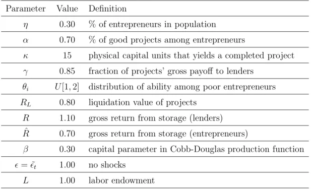
To advance one step further in the analysis, it is necessary to impose values to the parameters. Let us thus next configure a parametrical example for this Cobb-Douglas case. Those values are presented in Table 2.
Table 2: Choice of parameters Parameter Value Definition
η 0.30 % of entrepreneurs in population
α 0.70 % of good projects among entrepreneurs
κ 15 physical capital units that yields a completed project γ 0.85 fraction of projects’ gross payoff to lenders
θi U[1,2] distribution of ability among poor entrepreneurs
RL 0.80 liquidation value of projects
R 1.10 gross return from storage (lenders) ˆ
R 0.70 gross return from storage (entrepreneurs)
β 0.30 capital parameter in Cobb-Douglas production function = ˜t 1.00 no shocks
L 1.00 labor endowment
For this parameter configuration, all the imposed restrictions for existence of a SBC equilibrium are satisfied. This means that lenders fund all projects at the contracting stage, all poor entrepreneurs submit their projects for funding, and some of them gets refinancing at the interim stage. Given the assumptions we made to guarantee the existence of both good and poor projects, this analysis is restricted for an interval of capital kt∈(kmin, kmax).
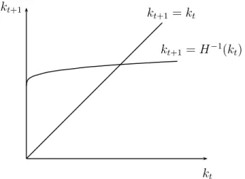
Using equation (20) with kt = kt+1 = kss, ˜t = and our parameter set, we
found that there exists a unique deterministic steady state (see Figure 6), and that kss ∈ (k
min, kmax). Moreover, this steady state is characterized by the presence
of soft budget constraint refinancing of poor entrepreneurs. Further simulations have revealed that those results are quiet robust to the parameter choice. We wanted to know how well this model behaves when we modify some key param-eters. In particular, we have conducted examples varying the parameter α that accounts for the proportion of good projects in the population of entrepreneurs. Starting from the initial 70% we used above, we have decreased αby ten
percent-kt+1
kt
kt+1 =kt
kt+1 =H−1(kt)
Figure 6: Intertemporal equilibrium existence - SBC case
age points at each time, and we found existence of steady states with soft budget constraint equilibria, even for a low 40% of good projects. For lower values of α, the participation constraint of lenders at the contracting stage is not satisfied. We have also modified the parameterη, the percentage of entrepreneurs in the to-tal population. This resulted in a more constrained range: steady state existence with soft budget constraint is guaranteed for η ∈ [0.2,0.3]. Finally, combining both ranges i.e. α ∈ [0.4,0.7] and η ∈ [0.2,0.3], we still find existence. We con-clude then that there exists a relatively large range of two crucial parameters for which there exists steady states characterized by soft budget constraint.
3.3
Econometric specification
In this section we analyze empirically a prediction of the model, the fact that the response of credit facing output expansions is larger inSBC economies compared to economies in which constraints are “hard”. To do that we propose a panel of 32 countries for the 1972-1999 period, with annual data. The data is presented in Table 3, countries include developed economies, Latin American countries and
South East Asia countries.
Credit (C) –expressed in local currency in current terms– comprises claims on the nonbanking private sector by commercial banks and other financial institutions, lines 22d and 42d of International Financial Statistics, IMF. The Gross Domestic Product (Y) is also obtained from IFS (line 99d). We denote the growth rate of real GDP per capita as ∆ ln Yi,t, using data from the Penn World Table.
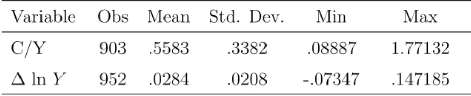
Descriptive statistics are presented in Table 3.
Table 3: Descriptive statistics
Variable Obs Mean Std. Dev. Min Max
C/Y 903 .5583 .3382 .08887 1.77132
∆ lnY 952 .0284 .0208 -.07347 .147185
Countries: Australia, Belgium, Canada, Denmark, Finland, France, Germany, Ireland, Israel, Italy, Japan, Netherlands, New Zealand, Norway, Spain, Sweden, Switzerland, UK, USA. Argentina, Brazil, Chile, Colombia, Mexico, Paraguay, Peru, Uruguay, Venezuela. Indonesia, Korea, Malaysia, Philippines, Singapore, Thailand.
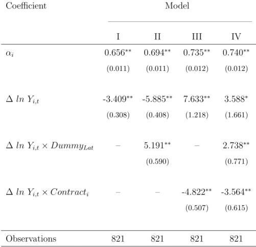
We run the following regression, using the Fixed Effects model:
(C/Y)i,t =αi+β1∆ln Yi,t+β2(∆ln Yi,t×DummyLat)+β3(∆ln Yi,t×Contracti)+ui,t
We explain the credit to GDP ratio using per capita GDP growth. This al-lows to control for the impact of rapidly growing economies on the demand for credit. Since in our model the SBC phenomenon arises in economies with low lev-els of screening and monitoring, we consider that this can have been the case for many Latin American countries. We then include the variable DummyLat which
adopts the value one for these countries, expecting to obtain higher responses of the Credit to GDP ratio facing output booms, i.e. β2 >0.
Table 4: Explaining the Credit to GDP ratio Dependent variable: Credit to GDP ratio, 1972-1999
Coefficient Model ———————————————— I II III IV αi 0.656∗∗ 0.694∗∗ 0.735∗∗ 0.740∗∗ (0.011) (0.011) (0.012) (0.012) ∆ ln Yi,t -3.409∗∗ -5.885∗∗ 7.633∗∗ 3.588∗ (0.308) (0.408) (1.218) (1.661)
∆ ln Yi,t×DummyLat – 5.191∗∗ – 2.738∗∗
(0.590) (0.771)
∆ ln Yi,t×Contracti – – -4.822∗∗ -3.564∗∗
(0.507) (0.615)
Observations 821 821 821 821
We also include the crossed variable (∆ ln Yi,t ×Contracti), where
“Con-tract” measures the relative degree to which contractual agreements are honored and complications presented by language and mentality differences. Scored 0-4, with higher scores for superior quality; average over 1980-95; Source: Knack and Keefer (1995), using data from Business Environmental Risk Intelligence (BERI). We guess that a better institutional framework, captured by higher val-ues of “Contract”, would be translated by a lower response of the Credit to GDP ratio. We are thus expecting the coefficient β3 to be negative. The results of this
regression are presented in Table 4, where we see we find the expected parame-ter signs: Latin American countries present a higher response of credit following
output growth, whereas the qualitative variable indicates countries with a better institutional environment show a lower response of credit.
4
Conclusions
We have constructed a model in which soft budget constraint phenomena appear as a result of adverse selection in credit markets. Any ex-ante liquidation threat by the part of lenders may not be credible for some levels of entrepreneurial sav-ings, which determines that poor projects are submitted to funding and some of them get refinancing. The model then reproduces one of the main ingredi-ents of this syndrome: when expectations of a future bailout are positive, then liquidations threats may not be credible enough so as to deter entrance of poor projects.
The main outcome of the model is to show the problem is more binding along the business cycle, i.e. when entrepreneurs net worth is high. The fraction of poor projects that is refinanced, total credit, investment, and the size of the bailout, are all increasing functions of entrepreneurial savings. This can be seen as further evidence to the rapid growth in the credit to the private sector that defines a lending boom, and to the increase in investment that accompanies such episodes.
Leaving the negative consequences of lending booms to the rest of the economy aside, we may ask: is all of this that bad? To answer this question, we have shown that in the soft budget constraint equilibrium the class of lenders loses in terms of second period consumption, compared to the perfect information equilibrium. Therefore, there is a cost in terms of welfare at least for some individuals.
The model is based on assumptions that best fit to economies with poor insti-tutions (no screening, no monitoring, weak enforcement of contracts). Therefore, when testing the main prediction of the model, we were expecting to find that countries with poorer institutional frameworks had higher responses of the credit to GDP ratio facing increases in GDP. Our guess was that Latin American coun-tries were an example of such councoun-tries, and the regression confirmed that. We
also found that the credit to GDP ratio overreact in a lower degree to changes in GDP in countries with a relative good environment for doing business.
Finally, policy recommendations are straightforward: concerning the environ-ment in which contracts are settled, regulation should be improved. At the same time, we could think on a tax to entrepreneurs. This would have the effect of lowering their savings during expansions to in turn decrease the proportion of poor projects that get refinancing.
References
[1] Aghion, Philippe; George-Marios Angeletos; Abhijit Banerjee and Kalina Manova (2005). “Volatility and Growth: Credit Constraints and Productivity-Enhancing Investment”. Mimeo. April.
[2] Azariadis, Costas and Shankha Chakraborty (1999). “Agency Costs in Dy-namic Economic Models”. The Economic Journal, Volume 109, April, pp 222-241.
[3] Bergara, Mario; Jorge Ponce and Leandro Zipitr´ıa (2003). “Institutions, Soft Budget Constraints and Bankruptcy”. Montevideo, Uruguay. Mimeo. July. [4] Bergl¨of, Erik and G´erard Roland (1997). “Soft budget constraints and credit
crunches in financial transitions”. European Economic Review, Volume 41, pp 807-917.
[5] Bernanke, Ben and Mark Gertler (1989). “Agency Costs, Net Worth, and Business Fluctuations”. American Economic Review, Volume 79, No. 1, March, pp 14-31.
[6] Dewatripont, Mathias and Eric Maskin (1995). “Credit and Efficiency in Cen-tralized and DecenCen-tralized Economies”. Review of Economic Studies, Volume 62, Issue 4, October, pp 541-555.
[7] Dewatripont, Mathias and G´erard Roland (1999). “Soft budget constraints, transitions and financial systems”. ECARE and CEPR. September.
[8] Gourinchas, Pierre Olivier; Oscar Landerretche and Rodrigo Vald´es (2001). “Lending Booms: Latin America and the World”. Econom´ıa (1) 2, Spring. [9] Kornai, Janos (1979). “Resource-Constrained Versus Demand-Constrained
Systems”. Econometrica. Volume 47, No. 4, pp 801-819.
[10] Kornai, Janos (1986). “The Soft Budget Constraint”. Kyklos, Blackwell Pub-lishing, vol. 39(1), pages 3-30.
[11] Kornai, Janos (1998). “The Place of the Soft Budget Constraint Syndrome in Economic Theory”. Journal of Comparative Economics. Volume 26, pp 11-17.
[12] Kornai, Janos; Eric Maskin and G´erard Roland (2003). “Understanding the Soft Budget Constraint”. Journal of Economic Literature, Volume 41, No. 4, December, pp 1095-1136(42).
[13] Mitchell, Janet (2000). “Theories of Soft Budget Constraints and the Anal-ysis of Banking Crises”. Economics of Transition, Volume 8 No. 1, March, pp 59-100.
[14] Vaz, Daniel (1999). “Four Banking Crises: Their Causes and Consequences”. Revista de Econom´ıa del Banco Central del Uruguay, Volume VI, No. 1, June.
A
Appendix
Proof of Proposition 3. Let us define the weightsδ, which express the fractions of lenders that finance projects (good and poor in all of its variants), or that simply use the storage technology:
• δ2(sEt ) =
(1−α)ησ(sE t )
1−η share of lenders who finance low-ability poor projects
(liquidation); • δ1(sEt ) =
(1−α)η(1−σ(sE t ))
1−η share of lenders who financehigh-ability Poor projects
(SBC);
• δ0 = 11−−2ηη share of lenders who simply store their savings.
Notice the dependence of δ1 and δ2 on entrepreneurial savings, since those are
functions of σ(sE
t ). The expected second period consumption of lenders in the
imperfect information case (cii
t+1) is thus given by
ciit+1 =δ3cGt+1+δ2ctP,low+1 +δ1cP,hight+1 +δ0cStort+1.
In turn, these expected levels of consumption are given by the sum of the gross payoffs from projects and from storage. In the case of funding a good project, the expected second-period consumption writes:
cGt+1 =γqˆt+1κ+R(st−1).
Those lenders that fundedlow-ability entrepreneurs (and hence their projects are liquidated at interim) get:
cP,lowt+1 =RL+R(st−1).
When lenders have funded a high-ability entrepreneur, the project is completed and thus their payoff is:
cP,hight+1 =γqˆt+1κ+R(st−1−
γqˆt+1κ−RL
R ) =RL+R(st−1).
Finally, for the case of lenders that can only store (no investment opportunities left for them):
cStort+1 =Rst.
Notice that
On the other hand, in the perfect information case (pi), lenders only fund good projects, so their expected second period consumption cpit+1 is given by
cpit+1 =δ3cGt+1+ (1−δ3)cStort+1.
We next show that the expected second period consumption of lenders is greater in the perfect information case: cpit+1 > cii
t+1, i.e.
δ3cGt+1+ (1−δ3)cStort+1 > δ3cGt+1+δ2cP,lowt+1 +δ1cP,hight+1 +δ0cStort+1 ,
which can be re written, using the above facts as
(1−δ3−δ0)cStort+1 >(δ1 +δ2)cP,lowt+1 ,
and (1−δ3−δ0) =δ1+δ2 so the above expression shrinks to
cStort+1 > cP,lowt+1 .
This condition holds by construction, then we have proven that cpit+1 > cii t+1. 2