Nils Holinski, Robert Vermeulen
The International Wealth Effect: A
Global Error-Correcting Analysis
The International Wealth Effect: A Global Error-Correcting
Analysis
∗Nils Holinskia , Robert Vermeulena,b
a
Department of Economics, Maastricht University, PO BOX 616, 6200 MD Maastricht b
Department of Economics, University of Luxembourg, 162A Avenue de la Faiencerie, L-1511 Luxembourg
April 27, 2009
Abstract
This paper analyzes the empirical link between asset prices, consumption and the trade balance using a global macroeconometric model developed by Pesaran, Schuermann, and Weiner (2004). The model is estimated for 29 countries with quarterly data over the period 1981Q1 - 2006Q4. Motivated by increasing international financial and real integration, and pronounced cycles in stock and housing prices, we employ generalized impulse response functions for a group of five of the world’s most industrialized countries and show that shocks to asset prices transmit into consumption decisions and subsequently into the trade balance. We refer to this transmission channel as the international wealth effect and find it to be present in the US, UK and, to a lesser extent, in France, but absent in Japan and Germany.
JEL Classification: E21, F15, F41, G15
Keywords: trade balance, wealth effect, global imbalances, GVAR, international transmission
∗
E-mail addresses: [email protected]; [email protected]. The authors thank seminar participants at Trinity College Dublin, DIW Macroeconometric Workshop in Berlin and NAKE Research Day in Utrecht for useful comments. They also thank Michel Beine, Bertrand Candelon, Clemens Kool, Joan Muysken and Jean-Pierre Urbain for constructive discussions. The second author gratefully acknowledges support by the Fonds National de Recherche Luxembourg under grant FNR/VIVRE/06/30/10.
1
Introduction
Households in the 1990s have witnessed substantial movements in their financial wealth, mainly owing to price changes in domestic and international stock markets. Over this decade, US and Scandinavian stock prices more than doubled in real terms, while many European countries experienced only moderate increases, and Asian countries, inflicted by the financial crisis in 1997, even saw considerable stock price decreases. At the end of the 1990s, stock markets culminated in the technology bubble, followed by its burst and plummeting stock prices in the early 2000s. Later, a remarkable and prolonged rebound set in which lasted until the recent outbreak of the subprime mortgage crisis in the US. As stock market wealth comprises the majority of most household’s financial assets, housing wealth generally comprises the majority of non-financial assets. Although most countries shared a marked and almost exponential increase in housing prices over the past ten years, housing wealth was also exposed to country-individual cycles.1
Much research emanates from this background and pursues the question of how these pro-nounced swings in financial and non-financial household wealth affect consumption decisions. This question refers to the so-calledconsumption-wealth effect ordomestic wealth effect, which is theoretically motivated by Friedman’s (1957) work on the consumption function and Modigliani’s and Brumberg’s (1954) life cycle consumption hypothesis. Empirical work on quantifying the impact of wealth on consumption dates back to the early contribution of Ando and Modigliani (1963) and has generated much interest among academics and policymakers thereafter.2
The objective of the present paper is to take up the domestic wealth effect and empirically link it to the trade balance. Considering the process of international integration of financial and real markets, we have all reasons to believe that changes in stock and housing prices affect not only consumption decisions through the domestic wealth effect, but further transmit into countries’ decisions on importing and exporting goods and services. We refer to this link where asset price movements are transmitted to the trade balance via consumption decisions as the
international wealth effect and investigate it for a group of five of the world’s most industrialized economies (G5) - the US, UK, Japan, Germany and France. We are particularly interested in the relative strength of the international wealth effect and test whether or not it can emerge as a potent alternative to the traditional exchange rate channel in correcting global current account imbalances.
Both theories, Friedman (1957) and Modigliani and Brumberg (1954), have in common that households consume out of their discounted value of total lifetime resources. That is, they smooth consumption over their life span by borrowing against future income when they are young, accumulating wealth during working age through saving and running down their wealth in retirement. Hence, any unexpected change in household wealth that is perceived as permanent will trigger households to adjust their consumption plans by a fraction of this change in wealth. The marginal propensity to consume out of different forms of household wealth is ultimately an
1
A notable exception is Switzerland, which experienced a stagnating housing market prior to the subprime mortgage crisis.
2
empirical issue and it has been found to be larger if the asset meets one or more of the following criteria: (1) the asset is liquid, (2) its value is easy to determine, (3) it is deemed appropriate to finance consumption and (4) the price change is considered to be permanent and certain.
Considering these criteria, it is not clear a priori if consumption is more responsive to changes in stock market or housing wealth. The first three criteria seem more applicable to stock market wealth (although mortgage deregulations make it increasingly possible to extract wealth from houses), while the last criterion is more applicable to housing wealth. A number of recent empirical studies on the domestic wealth effect find mixed evidence. They can be sorted along two dimensions: first, whether they address a single country, the US, (e.g. Ludvigson and Steindel, 1999; Mehra, 2001; Lettau and Ludvigson, 2004), or a panel of countries (e.g. Ludwig and Sløk, 2004; Case et al., 2005), and second, whether they distinguish between different forms of household wealth (e.g. Ludwig and Sløk, 2004; Case et al., 2005) or consider aggregated wealth only (e.g. Ludvigson and Steindel, 1999; Lettau and Ludvigson, 2001, 2004). We will review each dimension in turn.
Ludvigson and Steindel (1999) and Mehra (2001) employ cointegration techniques to study the domestic wealth effect in the US with quarterly data over the time period 1953 to 1997 and 1959 to 2000, respectively. They both arrive at the result that a dollar increase in wealth leads to a 3 to 5 percent increase in aggregate consumption. Moreover, Ludvigson and Steindel (1999) emphasize that the impact of movements in wealth appear to affect consumption con-temporaneously and not with a lag. Lettau and Ludvigson (2001, 2004) argue in their studies that the linkage between wealth and consumption cannot be understood without distinguishing between permanent and transitory movements. Using a cointegration framework that allows discriminating permanent from transitory behavior, they find for the US that only permanent movements in wealth affect aggregate consumption in the range of the aforementioned 3 to 5 percent. Case et al. (2005) extend the analysis to a panel of 14 countries and distinguish between stock market and housing wealth. They find at best a weak effect of stock market wealth on consumption, but strong evidence of a housing wealth effect. The estimated marginal propensity to consume out of housing wealth ranges between 11 to 14 percent. On the other hand, Ludwig and Sløk (2004) find no clear evidence that the responsiveness of consumption differs between changes in stock market and housing wealth for a panel of 16 OECD countries. However, they report that the structure of the financial system and the time period considered are decisive determinants for the estimated marginal propensity to consume out of wealth. Economies with market-based financial systems report on average higher marginal propensities than economies with bank-based financial systems. Moreover, the marginal propensity is found to be higher in the period between 1985 to 2000 as compared to the earlier years between 1960 to 1984.
We argue in the present paper that real and financial integration provoke an international perspective. Real integration, for instance the removal of barriers in trade of goods and services, brings about changes in aggregate consumption that impact not only the given country’s trade balance, but those of its trading partner as well. In addition, financial integration implies that countries hold a considerable share of their aggregate wealth in foreign assets, for instance
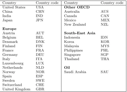
one-third of worldwide equity market capitalization was owned by foreign investors in 2006. In the same vein, mortgage securitization allows investors to easily participate in foreign housing mar-kets without actually owning property. All this bears the consequence, that, if stock or housing prices move in one country, it will affect the configuration of wealth positions across borders. In order to account properly for this new macroeconomic order, we base our empirical study of the international wealth effect on the global vector autoregression (GVAR) model introduced by Pesaran et al. (2004) - hereafter PSW - and advanced in Dees et al. (2007). Following PSW, we first capture the impact of movements in stock market and housing wealth on consumption and the trade balance by estimating country-individual vector error-correcting models (VECM). In addition to relevant domestic variables, we include the corresponding weakly-exogenous, trade-weighted foreign variables in these models. They fulfill two purposes: first, they proxy global unobserved common factors that serve as important international transmission channels, and second, they allow simultaneously solving the country-specific VECMs into an error-correcting GVAR representation. We proceed accordingly and first estimate a total of 29 country-specific VECMs with data at quarterly frequency over the time period 1981Q1 to 2006Q4. The models cover all countries and regions that figure prominently in the current debate on global imbal-ances - the US, China, Europe, Asia and oil-exporting countries. A complete list of the included countries is presented in Table 1.
[Table 1 about here.]
Next, we combine the country-individual models into a single error-correcting GVAR which allows studying the international wealth effect with an explicit account of the complex inter-national transmission channels of an integrated world. To date, empirical evidence on the international wealth effect is scarce. Despite the potential importance of asset prices for inter-national trade balance positions, we are aware of only one previous study that addresses the issue. Fratzscher et al. (2007) investigate the relative importance of stock market and housing prices for the US current account.3 Using a Bayesian structural vector autoregressive model, they find that asset prices account for up to 32 percent of movements of the US trade balance, while real exchange rates explain only around 7 percent and at shorter horizons. Their results suggest that the international wealth effect exerts considerable influence on the external adjust-ment process of the US. To account for the international dimension, they define US variables in differences to proxy for the rest of the world. Our empirical methodology is therefore much more comprehensive than the one by Fratzscher et al. (2007). Instead of leaving the rest of the world unmodeled, our GVAR methodology explicitly accounts for the rest of the world by means of the 29 country models. Considering, for instance, a shock to US asset markets, we allow for the possibility that the shock translates into the asset markets, and subsequently con-sumption decisions, of the other 28 countries from where it potentially feeds back into the US trade balance.
An alternative channel through which asset prices transmit to the trade balance of a country is worth considering here. This alternative channel of transmission is business and private expenditures on investments. The theoretical roots of this alternative are based on Tobin’s
q-theory of business investment. It says that firms find it worthwhile to invest in their capital stock in bullish asset markets as the ratio between the market value and the replacement value of its capital stock increases (Tobin, 1969). Moreover the financing of business investment is facilitated during these times. Also, the q-theory can be generalized to private housing investment and explain how shocks to real housing prices transmit to the trade balance without affecting consumption decisions.
Although we do not explicitly model this alternative transmission channel, we are aware of it when testing for the domestic and international wealth effect for the G5 countries. For each country, we expose stock market and housing prices to a negative shock and integrate out how consumption and the trade balance respond. To put these responses into perspective, we also consider a depreciating shock to the real effective exchange rate. This allows further insight into whether asset price movements emerge as a credible alternative to the exchange rate channel for the external adjustment process of a country. In addition, we conduct a variance-decomposition to assess the relevance of exchange rate, stock price and housing price movements on variations in the trade balance and consumption. An interesting question will be if our empirical methodology confirms the results of Fratzscher et al. (2007) for the US and whether or not they can be generalized to the G5 countries.
To preview the results of the present paper, our main findings are: first, movements in the real effective exchange rate affect consumption decisions only in the US. This points at the prominent role that the foreign sector plays for US consumption. Second, the domestic and international wealth effect, following a shock to domestic real stock prices, can not be generalized. They are at work in the US, UK and, to a lesser extent, in France but cannot be confirmed for Germany and Japan. Third, we observe an improving trade balance in the US, UK and France, following a negative shock to domestic real housing prices. It seems, however, that movements in housing prices do not transmit to the trade balance via the international wealth effect, but are possibly induced by business and private expenditures on investments. Fourth, in relative terms, domestic stock and housing prices exert at least as much influence on the trade balance as the real effective exchange rate does.
The rest of the paper is organized as follows. Section 2 sets out the empirical setup and the data series that we have used. Section 3 analyzes the dynamic properties of our model by means of impulse response functions, while Section 4 shows the corresponding forecast error variance decomposition. In Section 5 we expose our models to stability tests as a robustness check. Section 6 concludes.
2
Constructing the GVAR model
In this section, we first motivate the variables that are included in the country-individual models and discuss data considerations. Next we briefly outline the GVAR methodology and then address a number of issues that surround the proper fitting of the models to the data generation process.4
2.1 Variable selection and data considerations
The inclusion of variables in the country-individual models is guided by simple aggregate demand functions of open economy models.5 Moreover, we subject the models to a number of
specifica-tion tests to ensure reliable inference on all included variables. We consider the followingki×1
vector of endogenous variables,
yit= [tbit rcit ryit reerit rsit rhit rits rlit poilit ]0.6 (1)
for the country-individual VECM,i. The trade balance (tbit) is defined as the log of exports over
imports; real consumption (rcit) is the log of household consumption deflated by the consumer
price index; real gross domestic product (ryit) is the log of nominal gross domestic product
deflated by the consumer price index; the real effective exchange rate (reerit) is expressed in
logs; real stock market prices (rsit) are the log of a broad stock market index deflated by the
consumer price index; real housing prices (rhit) are the log of a housing price index deflated by
the consumer price index; the short term real interest rate (rits) is the log of a three-month money market rate deflated by the consumer price index and adjusted for quarterly frequency and the real long term interest rate (ritl) is the log of the rate on ten-year government bonds deflated by the consumer price index and adjusted for quarterly frequency. A notable exception constitutes the treatment of the oil price (poil
it ), which controls for global political events as an observable
common factor to all countries in our sample. Despite the growing importance of other regions in the world, we follow Dees et al. (2007) and includepoilit as an endogenous variable only in the US model, while retaining it as weakly-exogenous in all other country models.
Note that we includeryitandrcit in the country models. We see at least two reasons for the
inclusion of both. First, it allows for careful study of the various transmission channels of shocks to asset prices and the exchange rate, e.g. we are able to observe how savings - the difference betweenryit andrcit - react to these shocks. Second, we seek to get a grip on the often leveled
criticism that the observed wealth effect is spurious. Poterba and Samwick (1995) argue for instance that observed correlations between asset prices and consumption stem from the fact that asset prices convey information about future income growth. Movements in financial and
4
For a full exposition of the GVAR methodology, we refer the interested reader to Pesaran et al. (2004) and Dees et al. (2007).
5See for instance, Obstfeld and Rogoff (1996) or Sørensen and Whitta-Jacobsen (2005) for a textbook treat-ment.
6Depending on the availability of data, we may include fewer variables in some country models. See appendix for data availability and sources.
non-financial household wealth are captured by rsit and rhit, respectively. The use of price
indices as proxies for household wealth can be viewed as a limitation of our analysis, but studies by Ludwig and Sløk (2004) and Fratzscher et al. (2007) confirm that differences to volume based proxies for wealth are immaterial in estimations. Moreover, price indices allow exploiting the quarterly frequency at which these data are available. In the academic debate about causes and solutions to recent global current account imbalances, recurrent arguments include necessary exchange rate adjustments (e.g Blanchard et al. (2005), Holinski et al. (2009)) and relative output growth rates due to productivity differentials (e.g. Corsetti et al. (2008), Bems et al. (2007)). We control for these arguments with the variablesreeritandryit. Moreover, we decided
to include rits and rlit in the country models since specification tests show their importance for a sound modeling of stock market and housing prices. Additionally, by including both we allow for possible effects of bond markets.
In order to link the individual country-models and create international transmission channels, we match the domestic variables with trade-weighted foreign variables. The foreign variables remain unmodeled in the country models and thus need to satisfy weak exogeneity requirements for inference and impulse response analysis. We test and elaborate on the weak-exogeneity condition below. Theki∗×1 vector of foreign variables is denoted by
yit∗ = [rc∗it ryit∗ rs∗it rhit∗ rsit∗ rlit∗ poilit ]0 (2) and constructed as trade-weighted averages
rc∗it = N X j=1 wrcijrcjt ryit∗ = N X j=1 wryijryjt rs∗it= N X j=1 wrsijrsjt rh∗it = N X j=1 wrhijrhjt rs ∗ it = N X j=1 wijrsrsjt ritl∗= N X j=1 wrijlrljt (3)
where the country-specific trade-weights,wrcij, wryij, wrsij, wrhij, wijrs and wrijl fori, j = 1,2, ...N, are the sum of bilateral exports and imports between countryiand j relative to total exports and imports of country i.7 We employ time-invariant trade-weights in the construction of foreign
variables, which we obtain as averages over the years 2000 - 2004. Obviously, the correct choice of the weights is key in creating the international transmission channels. The use of information on bilateral trade in goods and services seems to be the natural choice for our study of the international wealth effect. An alternative choice is information on bilateral capital flows. However, data are not consistently available for all countries in our sample and we do not expect significant differences. The literature on the geography of portfolio investment shows that underlying trade in goods and services are key correlates for the observed patterns of capital flows (Portes and Rey, 2005; Lane and Milesi-Ferretti, 2008). The 29x29 trade share matrix that has been used in constructing the country-specific foreign variables are provided in Table
7
2 below.
[Table 2 about here.]
2.2 The GVAR methodology
The GVAR methodology proceeds in two stages. The first stage is the estimation stage of the following reduced form augmented vector autoregression, VARX(p, q), model for each countryi
in our sample yit=δi0+δi1t+ p X l=1 Φilyi,t−l+ q X m=0 Ψimyi,t∗ −m+it, i= 1,2, ..., N, t= 1,2, ..., T (4)
where δi0 and δi1 are ki×1 coefficient vectors of the deterministic intercept and time trend.8
yit is aki×1 vector of country-specific variables with corresponding ki×ki matrices of lagged
coefficients, denoted by Φil. y∗it is a k∗i ×1 vector of trade-weighted foreign variables with
corresponding ki×ki∗ matrices of contemporaneous and lagged coefficients, denoted by Ψim. it is aki×1 vector of zero mean, idiosyncratic country-specific shocks, assumed to be serially
uncorrelated with time invariant covariance matrix Σii. We determine the order of the dynamic
specification according to the Akaike information criterion (AIC). To reduce the number of estimated parameters, we allow at maximum for a VARX(2,1) specification. The lag orders of the individual countries are reported in Table 3.
[Table 3 about here.]
The modeling approach is well-suited to deal with variables that are approximately integrated of order one, in which case the VARX(2,1) can be written and estimated in a compact error-correction representation as
∆yit=δi0+δi1t−(Ai−Bi−Ci)zi,t−1+Ψi0∆y∗i,t−Φi2∆yi,t−1+it (5)
where zit = yit y∗it ! , Ai = (Iki,−Ψi0), Bi = (Φi1,Ψi1), Ci= (Φi2,0ki∗).
Ai,Bi andCi are matrices of dimension ki×(ki+ki∗). The error-correcting properties of each
country model are thus summarized in theki×(ki+k∗i) matrix
Πi = (Ai−Bi−Ci)
where the rank,ri, of Πi determines the number of long-run relationships between domesticand
country-specific foreign variables,yi andy∗i. To identify the rank of the cointegrating space for
8
each country model, we use the trace test statistic which is known to be more robust to departures from normal errors than the maximum eigenvalue test (Cheung and Lai, 1993).9 The number of long-run relationships according to the trace test statistic is listed for each country in Table 3. Below we elaborate on the integration properties of our variables and the long-run relationships between them. Note that the contemporaneous dependence of the domestic variables, yit, on the foreign variables,y∗it, in (4) and (5) makes it necessary to solve the country-specific models simultaneously for all of the domestic variables, yit. This is the second stage of the GVAR methodology, where we cast the country-specific models into its global representation. First rewrite (5) as
Ai∆zit =δi0+δi1t−(Ai−Bi−Ci)zi,t−1−Φi2∆yi,t−1+it (6)
and stack the endogenous variables of all individual country models in a k×1 global variable vectoryt= (y1t,y2t. . .yN t)0 withk=PNi=1ki. Next stack the country individual models of (6)
and solve for the global VECM representation
F∆yt=δ0+δ1t−(F−G−H)yt−1+Φ2∆yt−1+t (7) where δ0 = δ10 δ20 .. . δN0 , δ1= δ11 δ21 .. . δN1 , φ2 = Φ12 Φ22 .. . ΦN2 , t= 1t 2t .. . N t , and F= A1W1 A2W2 .. . ANWN , G= B1W1 B2B2 .. . BNWN , H= C1W1 C2W2 .. . CNWN .
The Wis are country-specific (ki +k∗i)×k matrices of fixed constants defined by the
trade--weights that were used above in the construction of the foreign variables. Wi is best thought
of as the link matrix that allows the country individual models to be written in terms of the global variable vector, yt. The global VECM of (7) allows for interaction among the included
economies through three different but interrelated channels: (1) the contemporaneous depen-dence of domestic variables, yit, on foreign variables, y∗it, and on its lagged values, (2) the dependence of all endogenous variables on common global exogenous variables (e.g. oil price), and (3) the nonzero contemporaneous dependence of shocks in country ion shocks in country
j. Cross-country shocks are allowed to be weakly correlated in Σij.
9
Departure from normal errors is particularly relevant in our study which includes equity and housing prices, interest rates and the real effective exchange rate.
Note that in the global VECM representation, domestic variables are no longer contempora-neously dependent on foreign variables. This implies that we can solve the global model forward recursively, obtain future values of all endogenous variables and conduct impulse response anal-ysis. We do so in Section 3. Before, we have a closer look at the statistical properties of the data series that we include in our model.
2.3 Properties and specification of the data series
As a first step in specifying the country individual model, we have to determine the integration properties of the included variables. The error-correction representation of the GVAR method-ology assumes that the included variables are approximately integrated of order one. We follow PSW and base our unit root tests on weighted symmetric estimations of ADF type regressions that possess superior power performance compared to standard ADF tests (Park and Fuller, 1995).
[Table 4 about here.] [Table 5 about here.]
Tables 4 and 5 present unit roott−statistics for the levels, first and second differences of the country-specific endogenous variables. The lag length of the tests is selected according to the AIC. The test results largely confirm well known results from previous literature. Real consump-tion, real output, real effective exchange rates and real stock and oil prices are unambiguously
I(1) processes for the vast majority of countries, or else I(0)/I(1) borderline cases. A different picture emerges for the unit root tests of the trade balances. Here, we find for a number of countries stationary data series, however, the trade balances of our focus countries are unam-biguously I(1). The real housing price series are I(1) processes with four notable exceptions: the US, Belgium, the Netherlands and Sweden. For these countries, we observe an exponential increase in housing prices over the past years of the sample period that renders the processes
I(2). Reducing the sample period by the last eight quarters produces I(1) real housing price processes for all countries in our sample. From the impulse response analysis below and the eigenvalues of the GVAR model we can conclude that the found integration order of housing prices does not impair the model’s stability. Finally, the hypothesis that interest rates areI(1) is rejected for many countries and may result in an efficiency loss in estimation. Overall, how-ever, it seems appropriate for our modeling strategy to treat all variables as approximatelyI(1). The estimation of the country individual models and the impulse response analysis below lend credibility to this conclusion.
Having established the integration properties, we proceed with specifying the number of long run cointegrating relationships that exist between domesticandforeign variables in each country model. Empirical evidence in the literature provides suggestions. Lettau and Ludvigson (2001) find a cointegrating vector between consumption, wealth and personal income for the US. Case and Shiller (2003) and Black et al. (2006) document cointegrating relationships between housing
prices, income and interest rates for the US. Specifically, Case and Shiller (2003) find stable price/income ratios for over forty US states. There is some evidence that international stock markets are cointegrated (Kasa, 1992), but these results are challenged by Richards (1995). Meese and Rogoff (1988) investigate the cointegrating properties of real exchange rates and real interest rate differentials, but reject a stable relationship between both variables. On the other hand, Bergvall (2004) finds a single cointegrating relationship between the trade balance, exchange rates, relative GDP and the real oil price for Scandinavian countries. Based on the trace statistic, Table 3 shows the number of cointegrating relationships in our country models. The number ranges from 1 for India to 6 for Sweden, but for the great majority of countries, including our G5 countries, we find 3 to 4 cointegrating relationships.
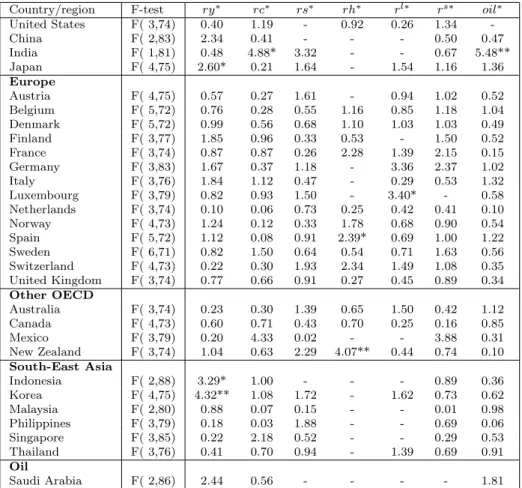
Finally, a key assumption underlying our estimation strategy is the weak exogeneity of the country-specific foreign variables,y∗it. It is best understood as the statistical formalization of the standard assumption in the small open-economy literature where it is generally assumed that most economies are too small relative to the size of the world economy to have an impact on the latter. The weak exogeneity assumption rules out any long run feedback from the endogenous variables,yit, to the foreign variables, y∗itand can be formally tested following Johansen (1992) and Harbo et al. (1999). They provide an F−test for the joint significance of the estimated error-correcting terms of (5) in the marginal model of the country-specific foreign variables,y∗it. To test, for instance, the weak exogeneity of foreign real output in the US country model, we need to consider the joint hypothesis thatγU S,j = 0,j= 1,2,3 in the auxiliary regression
∆ry∗U S,t=δU S+ 3 X j=1 γU S,jECMU S,tj −1+ l X k=1 ξU S,k∆ryU S,t−k+ n X m=1 ϑU S,m∆ry∗U S,t−m+U S,t
where ECMU S,tj −1 are the three long-run relationships found in the US country model and ∆ryU S and ∆ry∗U S are defined above. Table 6 reports the F−statistics for all country-specific foreign variables based on the lag order of the underlying VAR model. We find 8 out of 172 cases to be statistically significant at the 5% nominal level. All other foreign variables pass the weak exogeneity test. For our study, it is reassuring that for our set of focus countries, weak exogeneity can only be rejected for foreign real output in the Japanese country model, while all other foreign variables are weakly exogenous.10 Given the size and importance of the US equity market, we exclude foreign real stock prices from the US country model because these cannot be considered as weakly exogenous.
[Table 6 about here.]
10
As a robustness check, we excluded those foreign variables that do not pass the weak exogeneity test from the country models. The differences in estimation are immaterial.
3
Generalized Impulse Response Analysis
The complex cross-border interdependencies that are an integral part of our global model are best summarized by investigating the dynamic response of the system to shocks in the error of a given variable. The analysis is carried out by making use of generalized impulse response functions (GIRF) which have been introduced by Koop et al. (1996) for non-linear systems and advanced by Pesaran and Shin (1998) for vector error-correcting systems. The GIRF is an alternative to the orthogonalized impulse response (OIR) function that is proposed in the traditional VAR literature (Sims, 1980). While OIR functions rely on a set of orthogonalized shocks, the GIRF considers the shock to an individual error and integrates out the effects of the other shocks based on the historically observed distribution of all errors. Unlike OIR functions, the GIRF neither requires imposing identification restrictions, nor is it variant to the ordering of the endogenous variables in the global vector, yt. Both are clearly important considerations in our model that considers a total of 204 endogenous variables in 29 country models.
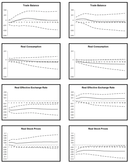
In what follows, we will investigate the time profiles and dynamic responses of domestic vari-ables to a one standard error negative shock to (1) the real effective exchange rate, (2) domestic real stock prices and, if available, (3) domestic real housing prices. We will focus mainly on the response of domestic consumption and the trade balance to investigate theinternational wealth effect transmission channel. The figures show the bootstrapped median impulse responses for the first 20 quarters following the shock together with the associated 90% confidence bounds.11 To stay focused we will concentrate on the G5 countries in the exposition of our results.
3.1 Domestic and international wealth effects in the US
The first column of Figure 1 shows the GIRFs for a one standard error negative shock to the US real effective exchange rate. This shock is equivalent to a currency depreciation of about 2% per quarter. The shock is highly persistent and thus the real effective exchange rate converges only slowly back to its mean as implied by long run PPP theory. The exchange rate depreciation leads to a statistically significant fall in real consumption of about 0.1% on impact and up to 0.4% after 20 quarters. Interestingly, the fall in consumption translates immediately into a statistically significant improvement of the US trade balance by about 0.3%. We do not observe the initial J-curve effect, which confirms previous studies (e.g Rose and Yellen, 1989). Taken together, the responses of real consumption and the trade balance lend support to the view that US trade balance deficits are, by and large, driven by US demand for imported goods and services. This view contrasts with Goldberg and Tille (2006) and Gust and Sheets (2006). Both studies argue that exchange rate movements are largely passed through to the trade balance via exports, leaving US expenditure on imports relatively unchanged.
[Figure 1 about here.]
11The confidence bounds are obtained using the sieve bootstrap procedure analagous to Dees et al. (2007) with 2000 replications.
Next, we expose US real stock prices to a one standard error negative shock. The associated GIRFs are shown in the second column of Figure 1. The shock amounts to a drop in real stock prices of 5-6% per quarter over the entire time horizon. The high persistence in the stock price behaviour following an initial shock can be attributed to the data series being integrated of order unity. Most importantly, on impact and over time we observe the domestic and international wealth effect at work. US real consumption falls by 0.1% on impact, by 0.5% after 4 quarters and by 0.7% after 20 quarters. The response of US real consumption is statistically significant throughout. As hypothesized, the domestic wealth effect becomes international - the fall in real consumption transmits into the US trade balance. Initially, the US trade balance improves by 0.3%, but it improves further by up to 1.7% after 8 quarters. The trade balance improvement is statistically significant over the first 12 quarters.
Note that real housing prices deteriorate significantly following a negative stock market shock. This decrease becomes significant after about eight quarters and remains significant after twenty quarters. The combined decrease in stock and housing prices may explain the strong effect of the stock market shock on consumption and consequently on the trade balance.
Finally, in the third column of Figure 1 a similar, yet less pronounced and statistically significant picture emerges for a one standard error negative shock to US real housing prices. The shock to US housing prices implies initially a 0.5% price decrease that stabilizes as a price decrease of about 1.5% over time. We observe that US real consumption turns negative after four quarters by up to 0.2%. However, the decrease in consumption ceases to be statistically significant. On the contrary, the trade balance improves following the negative shock to US real housing prices by 1.3% after 20 quarters and is statistically significant between quarters 1 and 10. Given the insignificant response of US real consumption, the transmission channel of housing price movements to the US trade balance, and thus evidence for the domestic and international wealth effect, is less clear cut. We conjecture that private and business investments are likely transmission channels.
When comparing the relevance of the real effective exchange rate and real stock and housing prices for the US trade balance, we find that all three variables bear equal importance. A one standard error negative shock to any variable improves the US trade balance on impact, and, even more over time (between 1.3% to 1.5%).
3.2 Domestic and international wealth effects in the UK
In the first column of Figure 2, we show the GIRFs of a one standard error negative shock to the UK real effective exchange rate. The shock results in a 2% depreciation of the UK real effective exchange rate per quarter. The depreciation is persistent over time. Unlike in the US, we do not observe a statistically significant effect of the relative price change on UK real consumption. This suggests that the foreign sector plays a less pivotal role for UK consumption decisisons than it does for the US. Also, the UK trade balance is less responsive to real effective exchange rate changes than the trade balance in the US. We find the classical J-curve behavior of the UK trade balance in response to a real effective exchange rate depreciation - an initial worsening
over the first 3 quarters followed by an improvement over the subsequent 11 quarters. Note, however, that the trade balance response is not statistically significant at any point in time.
[Figure 2 about here.]
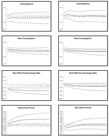
The shock to the real effective exchange rate serves as a benchmark against which we now evaluate shocks to UK real stock and housing prices. The second column of Figure 2 shows the GIRFs of a one standard error negative shock to UK stock prices. The shock implies a fall in stock prices of about 3.3% on impact, 2.7% after 4 quarters and 1.8% after 20 quarters. Similar to the US, we observe the domestic and international wealth effects at work for the UK. The fall in stock prices translates on impact into a statistically significant contraction of UK real consumption of about 0.1%, from where it further accelerates to 0.6% after 4 quarters and 0.7% after 20 quarters. The contraction is statistically significant over the entire time horizon. By way of comparison, we find the domestic wealth effect in the UK to be of the same order of magnitude as in the US.
Also, for a one standard deviation negative shock to UK real housing prices, we observe responses of UK real consumption and the UK trade balance that are, by and large, comparable to the respective responses in the US. The associated GIRFs are shown in the third column of Figure 2. The shock amounts to a fall in UK real housing prices of about 1.2% on impact and up to 2.2% after 5 quarters. On impact, the shock to real housing prices leads to the same statistically significant contraction of UK consumption as the shock to real stock prices - in both cases about 0.1%. Over time, however, UK real consumption continues to contract by about 0.1-0.2%, but its statistical significance ceases after the second quarter. This is reminiscent of the US real consumption response to the shock in real US housing prices. Similarly, we find that the UK trade balance improves considerably following the negative shock to UK real housing prices - in quarters 7 and 8 by up to 0.7%. The trade balance improvement is statistically significant between quarters 2 and 11. Again, a likely transmission channel are private and business expenditures on investments.
As with the US, we find that responses of UK real consumption and its trade balance to shocks to real stock and housing prices provide support for the existence of the domestic and international wealth effects. Unlike with the US, however, we observe that movements in the real effective exchange rate have neither a significant impact on UK consumption decisions, nor on the UK trade balance.
3.3 Domestic and international wealth effects in France
Similar to the two preceding countries, we also investigate for France the responses to a one standard negative shock to the French real effective exchange rate and compare it to the re-spective responses that are induced by shocks to French real stock and housing prices. The first column of Figure 3 shows the GIRFs of the negative shock to the French real effective exchange rate. The one standard error corresponds to an exchange rate depreciation of 1.2% on impact. Over time, the depreciation settles around 1.6%. Like before, we can attribute the persistence
of the shock to the integration property of the underlying data series. As with the UK, we do not observe a statistically significant effect of the real effective exchange rate change on French real consumption. We take from it that the dependence of US consumption on the relative prices of foreign goods and services is special. Furthermore, as for the UK, we observe that the French trade balance displays the aforementioned J-curve behavior without being statistically significant. These results are in line with Lee and Chinn (2006), who do not find a significant response of the French current account balance to a real exchange rate shock.
[Figure 3 about here.]
Columns 2 and 3 of Figure 3 show the GIRFs of one standard error negative shocks to French real stock and housing prices, respectively. The first shock implies a fall in French real stock prices of around 4.4% on impact and 3.7% over time. Again, we find the domestic and international wealth effects at work. Following the shock to domestic stock prices, French consumption contracts initially by 0.2%, and further by up to 0.4% in quarter 20. The statistical significance of the contraction ceases after 3 quarters. It is interesting to note that the response of French real consumption is about half of the respective response of real consumption in the US and UK and less statistically significant. This is suggestive of the finding that the domestic wealth effect is less pronounced for countries with bank-based, in contrast to market-based, financial systems (Ludwig and Sløk, 2004).
The one standard deviation negative shock to French real housing prices leads to a fall in real housing prices of 1.2% on impact that accelerates to 2.6% after 4 quarters and 4.1% after 20 quarters. The responses to the shock resemble, by and large, our findings for the US and UK. French real consumption contracts by 0.1 to 0.4%, but the contraction turns out to be statistically insignificant. At the same time, we observe an improved French trade balance of 0.3% on impact, 0.5% after 4 quarters and eventually 0.6% after 20 quarters. The response is statistically significant over the first 4 quarters and becomes marginally insignificant thereafter. Overall, the results for France are in line with what we have found for the US and UK. Movements in real effective exchange rates matter most for US real consumption and the US trade balance, less for the UK and France. Shocks to real stock prices unfold their domestic and international wealth effects for all three countries, but to a lesser extent for France. And finally, shocks to real housing prices transmit into the trade balances of all three countries, but real consumption does not seem to be the relevant channel.
3.4 Domestic and international wealth effects in Japan and Germany
We jointly present the results for Japan and Germany as for these countries real housing price data series are not available. The dynamic analysis is thus narrowed down to negative shocks of one standard deviation to the real effective exchange rates and real stock prices in both countries. The first column of Figure 4 shows the GIRFs for a negative shock to the real effective exchange rate of Japan. The shock corresponds to a depreciation of about 3% on impact and remains at this level after 20 quarters. While we observe that the depreciation of the exchange rate
translates into reduced real consumption, 0.07% after 4 quarters and 0.27% after 20 quarters, the response is statistically insignificant.
[Figure 4 about here.]
Similarly, the Japanese trade balance displays the classic J-curve behavior, which is only statistically significant on impact. Gupta-Kapoor and Ramakrishnan (1999) provide empirical evidence in favor of the existance of the J-curve for Japan. Next we expose Japanese real stock prices to a one standard deviation negative real stock price shock. It implies a fall in stock prices of 6.2% on impact and about 5.3% after a few quarters. The corresponding GIRFs are shown in the second column of Figure 4 and provide evidence for the existence of the domestic wealth effect, but fail to recognize the international wealth effect. Following the shock to Japanese real stock prices, we find that real consumption in Japan drops by 0.1% on impact, and further by up to 0.5% after 20 quarters. The drop is statistically significant over the first 10 quarters. However, the response of consumption does not translate into the Japanese trade balance. There, we do not observe any statistically significant change.
Figure 5 shows the GIRFs for one standard deviation negative shocks to the real effective exchange rate and real stock prices of Germany. For this country, we do not find the domestic or international wealth effects at work - real consumption and the trade balance do not change significantly following the shock to German real stock prices. Similarly, we find that the real effective exchange rate does not exert a significant influence on real consumption and the trade balance in Germany. The reunification of the country produced breaks in the first quarter of 1991 in most German data series. While the GVAR methodology copes with co-breaking data series, we also transformed the data series and included a dummy in the short-term dynamics of the model. The above described results are found to be robust across specifications.
[Figure 5 about here.]
4
Generalized forecast error variance decomposition
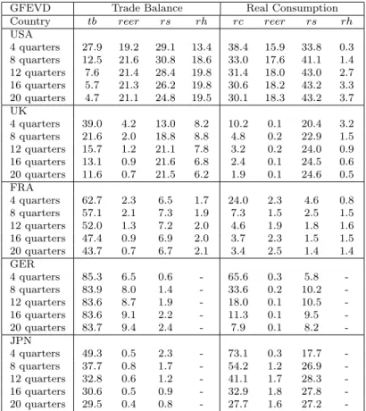
Complementary to the GIRF analysis in the previous section, we conduct a generalized forecast error variance decomposition (GFEVD) to answer the question of how much of the error variance in forecasting the trade balance and real consumption can be attributed to shocks in the real effective exchange rate, real stock market and real housing prices. The results are shown in Table 7 and strongly confirm our previous findings from the generalized impulse response analysis. They can be summarized as: first, shocks to the real effective exchange rate are by far most influential for real consumption and the trade balance in the US. Over all time horizons, these shocks explain up to 18.3% of the variation in real consumption and 21.6% of the variation in the trade balance. By contrast, in all other G5 countries, shocks to the real effective exchange rate contribute at most 2.5% to the variation in real consumption and 9.4% to the variation in the trade balance. Particularly, the pronounced impact that shocks to the real effective exchange
rate have on US consumption decisions provides a strong case for the prominent role that the foreign sector plays in the US.
[Table 7 about here.]
These results confirm the findings of Lane and Milesi-Ferretti (2002), who find a strong rela-tionship between the real exchange rate and the trade balance for the US, a weaker relarela-tionship for Germany and no connection for France and the UK. However, Lane and Milesi-Ferretti (2002) find a strong dependence of the Japanese trade balance on the real exchange rate, whereas we find that the real effective exchange rate does not play a role.
Second, except for Germany, we find in all other G5 countries that shocks to real stock prices explain a substantially greater share of the variation in real consumption and the trade balance than real effective exchange rates do. We take from it that domestic stock price movements constitute a potent alternative to the traditional exchange rate channel in shaping a country’s external adjustment process. The international wealth effect is a likely channel.
Third, in all G5 countries, shocks to real housing prices contribute a greater share to the forecast error variance of the trade balance than of real consumption. This points at the potential relevance of business and private investment decisions for passing through housing price shocks to the trade balance. The international wealth effect plays a subordinated role. And finally, the forecast error variance decomposition confirms the idiosyncratic behavior of the German trade balance and real consumption - about 84% of the variation in the trade balance and up to 66% of the variation in real consumption are explained by their own shocks.
5
Stability and specification of the global VAR
One of the underlying assumptions of the GVAR is structural stability of long-run coefficients, short-run coefficients and the error variances. In this setting the model faces problems in case of structural breaks. However, this is not a problem specific to the GVAR, but to macroeconometric models in general. Unfortunately, there is no consensus on how to best model breaks and there are no satisfactory methods available in the literature. So, our main aim is to construct a model as robust as possible to possible breaks. Dees et al. (2007) point out that the structural problem is reduced within the GVAR by the inclusion of foreign variables in the country-individual models. The GVAR is able to accommodate the so-called ‘co-breaking’, which should make it more robust to the possibility of structural breaks than reduced-form single-equation models.12
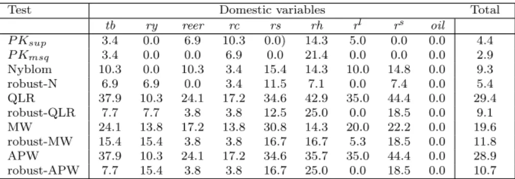
In order to address the concerns on structural stability, we conduct a battery of structural break tests to judge the (in-)stability of the coefficients. Following Dees et al. (2007), we consider structural stability tests that are based on the residuals of the individual equations of the country individual models. Here we use ten different stability tests: the Ploberger and Kr¨amer (1992) maximal OLS CUSUM statistic (PKsup), its mean square variant (PKmsq), the Nyblom (1989)
test (Nyblom), which considers a non-stationary alternative, the Wald form of the Quandt
12
(1960) likelihood ratio statistic (QLR), the mean Wald statistic (MW) of Hansen (1992) and Andrews and Ploberger (1994) and the Andrews and Ploberger (1994) Wald statistic based on the exponential average (APW). For the latter four tests we also apply the heteroskedastic-robust versions.
Table 8 shows the test results, where for each variable the percentage of rejections at the 5% nominal level is reported. The last column shows the total number of rejections by each test. When we consider the PKsup and PKmsq test the total rejection rate of parameter stability is
4.4% and 2.9%, respectively. This implies that we reject coefficient stability only for a small number of variables. The Nyblom test shows similar results, both versions show rejection rates lower than 10% and based on these results there seems to be little concern about parameter stability.
[Table 8 about here.]
Interestingly, the tests do not always reject stability for the same variables. The PK tests never reject stability for stock market prices, whereas the Nyblom tests show relatively high rejection rates. A similar story applies to short-term interest rates.
The QLR, MW and APW tests show very high rejection rates across all variables. Both the QLR and APW tests shows rejection rates of over 30% for stock prices, housing prices, short-term and long-term interest rates. The QLR rejects stability for 60 out of 204 variables and the results for MW and APW show similar rejection rates. However, the rejection rates are much lower when we take heteroskedasticity into account in these tests. Accounting for heteroskedasticity is especially important for variables such as stock and housing prices. In this situation all tests show rejection rates close to 10%. Notice that the drop is especially strong for those variables which had high rejection rates before accounting for heteroskedasticity.
These findings imply that the main reason of rejection by the tests appears to be breaks in error variances and not changes in the parameter coefficients. So, most of the structural parameters in our model seem to be relatively stable and concerns for structural breaks are mitigated. In line with Dees et al. (2007), we account for heteroskedasticity by using robust bootstrapped standard errors for the confidence bounds of the GIRFs and interpret the GIRFs conservatively by taking 90% confidence bounds.
6
Conclusion
In this paper we empirically test the link between real stock and housing prices, consumption and the trade balance. Against the background of an established theoretical and empirical literature that links asset prices to consumption through the domestic wealth effect, we argue that the current surge of real and financial integration provokes an international perspective. Hence, we hypothesize that movements in real stock and housing prices not only transmit into a country’s consumption decision, but further into the trade balance. We refer to this second link as the international wealth effect and test it using the recent GVAR methodology of PSW.
The GVAR methodology is particularly suited for our study since it explicitly accounts for the complex interdependencies that exist across countries. It proceeds in two steps. First, we estimate individual VECMs for 29 countries over the period 1981Q1-2006Q4. Second, we combine these country individual models into a global VAR representation using information on bilateral trade patterns. The global VAR model allows conducting generalized impulse response studies and forecast error variance decompositions that provide evidence in favor of the existence of the domestic and international wealth effect in the US, UK and France. In these countries, exposing real stock prices to a one standard deviation negative shock results in a statistically significant contraction of real consumption and improvement of the trade balance. Moreover we observe that the trade balances of the same countries improve following a negative shock to real housing prices. Since the shock is not transmitted through consumption, hence the international wealth effect, we conjecture that business and private expenditures on investments are the likely transmission channels. We also test the domestic and international wealth effect for Germany and Japan, but do not find any statistically significant results. To determine the relative importance of real stock and housing prices for consumption and the trade balance, we also consider the real effective exchange rate in our studies and find compelling evidence that asset prices are at least as important drivers of international trade balances as real effective exchange rates. This finding is a crucial impetus in the recent debate on global current account imbalances. In this context, we also find that movements in the real effective exchange rate exert a considerable influence on US real consumption and the trade balance. This influence is not paralleled by any other country and points at the prominent role that the foreign sector plays for the US.
References
Ando, A. and Modigliani, F. (1963). The Life-Cycle Hypothesis of Savings: Aggregate Implica-tions and Tests,The American Economic Review 103: 55–84.
Andrews, D. and Ploberger, W. (1994). Optimal Tests When a Nuisance Parameter is Present Only Under the Alternative, Econometrica62: 1383–1414.
Bems, R., Dedola, L. and Smets, F. (2007). US Imbalances: The Role of Technology and Policy,
Journal of International Money and Finance26: 523–545.
Bergvall, A. (2004). What Determines Real Exchange Rates? The Nordic Countries, Scandina-vian Journal of Economics106(2): 315–337.
Black, A., Hoesli, P. and Fraser, M. (2006). House Prices, Fundamentals and Bubbles,Journal of Business Finance & Accounting 33: 1535–1555.
Blanchard, O., Giavazzi, F. and Sa, F. (2005). The U.S. Current Account and the Dollar,
Brookings papers on Economic Activity1: 1–65.
Case, K. E., Quigley, J. M. and Shiller, R. J. (2005). Comparing Wealth Effects: The Stock Market versus the Housing Market,B. E. Advances in Macroeconomics5(1).
Case, K. E. and Shiller, R. J. (2003). Is There a Bubble in the Housing Market?, Brookings Papers on Economic Activity2003:2.
Cheung, Y. W. and Lai, K. S. (1993). Finite-Sample Sizes of Johansen’s Likelihood Ratio Test for Cointegration, Oxford Bulletin of Economics and Statistics 55: 313–328.
Corsetti, G., Dedola, L. and Leduc, S. (2008). Productivity, External Balance and Exchange Rates: Evidence on the Transmission Mechanism Among G7 Countries, The Review of Eco-nomic Studies 75: 443–473.
Dees, S., Di Mauro, F., Pesaran, M. H. and Smith, L. V. (2007). Exploring the International Linkages of the Euro Area: A Global VAR Analysis,Journal of Applied Econometrics 22: 1– 38.
Fratzscher, M., Juvenal, L. and Sarno, L. (2007). Asset Prices, Exchange Rates and the Current Account,ECB Working Paper Series No. 790.
Fratzscher, M. and Straub, R. (2009). Asset Prices and Current Account Fluctuations in G7 Economies, ECB Working Paper Series No. 1014.
Friedman, M. (1957). A Theory of the Consumption Function, NJ: Princeton University Press, Princeton.
Goldberg, L. and Tille, C. (2006). The Internationalization of the Dollar and Trade Balance Adjustment,Federal Reserve Bank of New York Staff Report255.
Gupta-Kapoor, A. and Ramakrishnan, U. (1999). Is There a J-Curve: A New Estimation for Japan,International Economic Journal 13: 71–79.
Gust, C. and Sheets, N. (2006). The Adjustment of Global External Imbalances: Does Partial Exchange Rate Pass-Through to Trade Prices Matter?, Federal Reserve Bank International Finance Discussion PapersNo. 855.
Hansen, B. E. (1992). Tests for Parameter Instability in Regressions With I(1) Processes,
Journal of Business & Economic Statistics 10: 321–336.
Harbo, I., Johansen, S., Nielsen, B. and Rahbek, A. (1999). Asymptotic Inference on Cointe-grating Rank in Partial Systems,Journal of Business & Economic Statistic 16: 388–399. Hendry, D. F. (1996). A Theory of Co-Breaking,mimeo, University of Oxford .
Hendry, D. F. and Mizon, G. E. (1998). Exogeneity, Causality and Co-Breaking in Economic Policy Analysis of a Small Econometric Model of Money in the UK, Empirical Economics
23: 267–294.
Holinski, N., Kool, C. and Muysken, J. (2009). International Portfolio Balance - Modeling the External Adjustment Process,mimeo, Maastricht University .
Johansen, S. (1992). Cointegration in Partial Systems and the Efficiency of Single-Equation Analysis,Journal of Econometrics52: 389–402.
Kasa, K. (1992). Common Stochastic Trends in International Stock Markets,Journal of Mon-etary Economics 29: 95–124.
Koop, G., Pesaran, M. H. and Potter, S. M. (1996). Impulse Response Analysis in Nonlinear Multivariate Models, Journal of Econometrics74: 119–147.
Lane, P. and Milesi-Ferretti, G. M. (2002). External Wealth, the Trade Balance, and the Real Exchange Rate, European Economic Review46: 1049–1071.
Lane, P. and Milesi-Ferretti, G. M. (2008). International Investment Patterns, The Review of Economics & Statistics 90(3): 538–549.
Lee, J. and Chinn, M. (2006). Current Account Dynamics and Real Exchange Rate Dynamics in G7 Countries,Journal of International Money and Finance 25: 257–274.
Lettau, M. and Ludvigson, S. (2001). Consumption, Aggregate Wealth, and Stock Returns,The Journal of Finance LVI(3): 815–849.
Lettau, M. and Ludvigson, S. (2004). Understanding Trend and Cycle in Asset Values: Reeval-uating the Wealth Effect on Consumption,The American Economic Review 94(1): 276–299. Ludvigson, S. and Steindel, C. (1999). How Important is the Stock Market Effect on
Ludwig, A. and Sløk, T. (2004). The Relationship Between Stock Prices, House Prices and Consumption in OECD Countries,Topics in Macroeconomics 4: 1–26.
Meese, R. and Rogoff, K. (1988). Was it Real? The Exchange Rate-Interest Differential Over the Modern Floating-Rate Period, The Journal of Finance43(4): 933–948.
Mehra, Y. P. (2001). The Wealth Effect in Empirical Life-Cycle Aggregate Consumption Equa-tions, Federal Reserve Bank of Richmond Economic Quarterly87(2): 45–68.
Modigliani, F. and Brumberg, R. (1954). Utility Analysis and the Consumption Function: An Interpretation of Cross-Section Data, Rutgers University Press, New Brunswick.
Nyblom, J. (1989). Testing For the Constancy of Parameters Over Time,Journal of the Amer-ican Statistical Association84: 223–230.
Obstfeld, M. and Rogoff, K. (1996). Foundations of International Macroeconomics, The MIT Press, Cambridge, Massachusetts, US.
Park, H. and Fuller, W. (1995). Alternative Estimators and Unit Root Tests for the Autore-gression Process, Journal of Time Series Analysis16: 415–429.
Pesaran, M. H., Schuermann, T. and Weiner, S. M. (2004). Modeling Regional Interdependencies Using a Global Error-Correcting Macroeconometric Model,Journal of Business & Economic Statistics22(2): 129–162.
Pesaran, M. H. and Shin, Y. (1998). Generalized Impulse Response Analysis in Linear Multi-variate Models,Economics Letters 58: 17–29.
Ploberger, W. and Kr¨amer, W. (1992). The CUSUM Test With OLS Residuals, Econometrica
60: 271–286.
Portes, R. and Rey, H. (2005). The Determinants of Cross-Border Equity Flows, Journal of International Economics65: 269–296.
Poterba, J. M. (2000). Stock Market Wealth and Consumption,Journal of Economic Perspective
13: 91–118.
Poterba, J. M. and Samwick, A. A. (1995). Stock Ownership Patterns, Stock Market Fluctua-tions, and Consumption,Brookings Papers on Economic Activity 2: 295–357.
Quandt, R. (1960). Tests of the Hypothesis that a Linear Regression System Obeys Two Separate Regimes,Journal of the American Statistical Association 55: 324–330.
Richards, A. (1995). Comovements in National Stock Market Returns: Evidence of Predictabil-ity, but Not Cointegration, Journal of Monetary Economics36: 631–654.
Rose, A. K. and Yellen, J. L. (1989). Is There a J-Curve?, Journal of Monetary Economics
Sims, C. (1980). Macroeconomics and Reality,Econometrica48: 1–48.
Sørensen, P. B. and Whitta-Jacobsen, H. J. (2005). Introducing Advanced Macroeconomics: Growth & Business Cycles, Mc Graw Hill, Maidenhead, UK.
Tobin, J. (1969). A General Equilibrium Approach to Monetary Theory, Journal of Money, Credit and Banking 1: 15–29.
Appendix: Data sources
• Trade data for all countries are from the IMF Direction of Trade Statistics at the quarterly frequency and in US$. The trade balance is constructed as the log of exports over imports and seasonally adjusted in EViews using the X12 method of the US Census Bureau.
• Nominal consumption, nominal output and inflation data are from the IMF International Financial Statistics at the quarterly frequency an in domestic currency. For China, India, Indonesia, Malaysia, New Zealand, Saudi Arabia and Thailand annual data are interpo-lated to a quarterly frequency in some cases. We interpolate the data by first taking logs and assuming a constant growth rate between two annual observations. Real consumption and real output are seasonally adjusted in EViews using the X12 method of the US Census Bureau.
• Real effective exchange rate data are taken from the IMF International Financial Statistics at the quarterly frequency.
• Stock price data are from Global Financial Data using a large domestic stock market index. Stock market index prices are denominated in local currencies and at the quarterly frequency.
– United States (S&P 500 Composite Price Index), Japan (Nikkei 225 Stock Average) and India (Bombay SE Sensitive Index)
– European countries: Austria (Wiener Boersekammer Share Index), Belgium (Brussels All-Share Price Index), Denmark (OMX Copenhagen All-Share Price Index), Finland (OMX Helsinki All-Share Price Index), France (SBF-250 Index), Germany (CDAX Composite Index), Italy (Banca Commerciale Italiana Index), Luxembourg (LuXX Index), Netherlands (All-Share Price Index), Norway (Oslo SE All-Share Index), Spain (Madrid SE General Index), Sweden (Affarsvarlden General Index) and United Kingdom (FTSE All-Share Index)
– Other OECD: Australia (ASX All-Ordinaries), Canada (S&P/TSX 300 Composite), Mexico (SE Indice de Precios y Cotizaciones) and New Zealand (SE Share Capital All Index)
– South-East Asia: Korea (SE Stock Price Index KOSPI), Malaysia (KLSE Composite), Philippines (Manila SE Composite Index), Singapore (FTSE All-Share Index) and Thailand (SET General Index)
• Housing price data are from the Bank of International Settlements at quarterly frequency.
• Both short term and long term interest rates are from the IMF International Financial Statistics at the quarterly frequency.
• The oil price is the price in US$ of one barrel Brent crude and retrieved through Datas-tream.
Table 1: Countries and regions in the model
Country Country code Country Country code United States USA Other OECD
China CHN Australia AUS
India IND Canada CAN
Japan JPN Mexico MEX
New Zealand NZL
Europe
Austria AUT South-East Asia
Belgium BEL Indonesia IDN
Denmark DNK Korea KOR
Finland FIN Malaysia MYS
France FRA Philippines PHL
Germany DEU Singapore SGP
Italy ITA Thailand THA
Luxembourg LUX
Netherlands NLD Oil
Norway NOR Saudi Arabia SAU
Spain ESP
Sweden SWE
Switzerland CHE United Kingdom GBR
T able 2: T rade w eigh t matrix Coun tr y/regi on USA CHN IND JPN A UT BEL DNK FIN FRA DEU IT A LUX NLD NOR ESP SWE CHE GBR A US CAN MEX NZL IDN K OR MYS PHL SGP THA SA U United States 0.0 10.1 1.0 11.4 0.4 1.5 0.3 0.3 3.1 5.8 2.2 0.1 1.9 0.5 0.8 0.9 1.2 4.9 1.2 24.4 14.8 0.3 0.8 3.9 2.2 1.2 2.1 1.4 1.4 China 22.9 0.0 1.2 24.2 0.3 1.2 0.4 0.7 2.3 6.8 2.1 0.1 2.6 0.3 0.9 0.8 0.7 2.8 2.6 2.0 0.8 0.3 1.9 10.9 3.1 1.3 3.4 2.1 1.2 India 21.2 7.1 0.0 5.9 0.4 7.4 0.5 0.4 3.1 6.7 3.5 0.0 2.2 0.3 1.5 1.0 4.4 8.1 3.2 1.8 0.5 0.2 3.1 3.6 3.5 0.6 5.1 1.7 2.7 Japan 28.9 17.2 0.7 0. 0 0.3 1.1 0.5 0.4 2.1 4.6 1.7 0.0 2.1 0.3 0.7 0.6 0.9 3.0 3.7 2.3 1.0 0.6 3.5 7.7 3.8 2.4 3.4 4.0 2.7 Europ e Austria 5.3 1.6 0.2 1.6 0.0 2.6 0.8 0.9 5.4 48.8 10.1 0.3 4.2 0.3 2.5 1.6 6.5 4.4 0.3 0.7 0.2 0.1 0.1 0.5 0.2 0.1 0.2 0.2 0.3 Belgium 7.7 1.9 1.5 2.3 1.0 0.0 0.7 0.7 17.8 21.1 5.5 1.5 16.8 0.7 3.4 2.1 1.2 10.1 0.4 0.7 0.3 0.1 0.3 0.5 0.2 0.1 0.3 0.5 0.2 Denmark 6.0 2.4 0.5 2.7 1.2 2.9 0.0 3.3 6.0 24.1 4.4 0.2 6.9 6.2 2.6 14.6 1.4 10.0 0.5 0.7 0.2 0.2 0.2 1.0 0.3 0.1 0.4 0.4 0.3 Finland 8.6 3.9 0.5 3.3 1.5 3.5 4.7 0.0 5.8 18.1 4.8 0.1 6.5 3.8 2.8 14.7 1.7 9.9 1.1 0.9 0.3 0.1 0.4 0.8 0.5 0.4 0.4 0.5 0.4 F rance 8.8 2.4 0.4 2.2 1.2 10.3 1.0 0. 7 0. 0 21.1 11.2 0.9 6.9 1.3 10.1 1.6 3.8 10.7 0.5 0.9 0.4 0.1 0.2 0.8 0.4 0.1 0.7 0.3 0.8 German y 11.7 4.2 0.6 3.8 6.1 6.6 2.2 1.4 13.3 0.0 9.1 0.5 9.5 1.8 5.1 2.6 5.2 9.8 0.6 0.9 0.7 0.1 0.4 1.2 0.7 0.3 0.9 0.5 0.4 Italy 9.4 3.2 0.7 2.6 3.3 4.9 1.0 0.8 16.2 22.0 0.0 0.4 5.8 0.7 7.7 1.6 5.0 8.1 0.9 1.0 0.6 0.1 0.4 1.2 0.4 0.1 0.5 0.4 1.0 Luxem b ourg 3.4 3.4 0.1 0.9 1.2 24.7 0.6 0. 5 17.1 25.8 4.3 0.0 5.0 0.2 2.6 1.1 1.7 5.9 0.1 0.4 0.1 0.0 0.2 0.3 0.1 0.1 0.1 0.1 0.1 Netherlands 7.9 3.4 0.4 2.9 1.3 13.1 1.4 1. 2 9. 5 26.2 5.3 0.3 0.0 1.4 3.5 2.4 1.5 10.8 0.4 0.6 0.3 0.1 0.5 0.9 1.2 0.7 1.1 0.6 0.9 Norw a y 8.4 2.4 0.2 2.5 0.5 2.9 5.7 2.8 9.2 13.8 3.3 0.1 9.0 0.0 2.1 11.8 0.8 17.9 0.2 4.0 0.1 0.0 0.1 1.0 0.2 0.1 0.6 0.2 0.1 Spain 5.4 2.6 0.5 2.2 1.4 4.3 1.0 0.8 24.0 19.3 12.0 0.2 5.7 0.7 0.0 1.6 1.7 10.3 0.4 0.6 1.6 0.1 0.6 1.0 0.3 0.1 0.3 0.4 1.0 Sw eden 9.7 2.4 0.6 2.8 1.3 5.0 8.6 6.6 6.3 16.3 4.2 0.2 6.9 9.7 2.7 0.0 1.5 9.9 0.8 0.9 0.5 0.1 0.3 0.7 0.5 0.1 0.5 0.4 0.6 Switzerland 10.8 1.9 0.5 3.7 4.2 2.9 0.9 0.7 11.6 30.5 11.0 0.2 4.8 0.3 3.2 1.4 0.0 6.0 0.5 0.9 0.5 0.1 0.2 0.7 0.3 0.1 0.8 0.6 0.6 United Kingdom 17.6 2.9 1.3 4.0 1.0 6.5 1.5 1.2 11.1 15.7 5.7 0.2 8.8 2.6 4.7 2.6 2.4 0.0 1.3 2.3 0.4 0.3 0.5 1.4 0.9 0.4 1.3 0.7 0.8 Other OECD Australia 16.4 10.5 1.9 18.5 0.4 0.9 0.4 0.6 2.2 4.4 2.8 0.0 1.3 0.2 0.8 1.0 0.8 5.6 0.0 1.7 0.5 6.1 3.4 6.6 3.4 0.9 4.5 2.8 1.6 Canada 79.2 3.1 0.3 3.3 0.2 0.4 0.2 0.2 1.1 1.6 0.8 0.0 0.4 0.7 0.3 0.3 0.3 2.3 0.4 0.0 2.2 0.1 0.2 1.0 0.4 0.2 0.2 0.3 0.2 Mexico 80.7 2.6 0.3 3.0 0.1 0.3 0.1 0.1 0.7 2.5 0.8 0.0 0.3 0.0 1.1 0.3 0.3 0.6 0.2 2.4 0.0 0.1 0.2 1.4 0.8 0.3 0.5 0.3 0.1 New Zealand 16.8 7.3 0.7 13.6 0.3 1.6 0.5 0.4 2.2 4.4 2.3 0.0 1.0 0.1 0.6 0.8 0.6 4.9 24.8 2.0 1. 0 0.0 1.6 3.8 2.7 1.1 1.9 1.7 1.3 South-East Asi a Indonesia 13.7 7.2 2.6 23.2 0.2 1.3 0.2 0.3 1.4 3.4 1.4 0.0 2.5 0.1 1.4 0.5 0.4 2.4 4.5 1.1 0.3 0.4 0.0 7.6 4.2 1.3 12.3 3.5 2.4 Korea 23.1 17.3 1.2 19.4 0.3 0.7 0.3 0.5 1.5 4.2 1.7 0.0 1.5 0.4 0.8 0.4 0.6 2.7 3.3 1.7 1.0 0.4 3.2 0.0 3.0 1.9 3.2 1.6 4.0 Mala ysia 21.4 7.2 1.9 17.4 0.2 0.6 0.2 0.2 1.6 3.6 0.8 0.0 2.9 0.1 0.4 0.5 0.7 2.7 2.6 0.7 0.5 0.4 3.1 4.7 0.0 2.5 17.4 5.1 0.7 Philippines 26.5 4.9 0.6 21.7 0.2 0.6 0.1 0.4 0.9 3.7 0.5 0.0 5.7 0.0 0.3 0.2 0.4 2.3 1.6 1.0 0.4 0.4 1.7 6.2 5.2 0.0 8.5 3.9 1.9 Singap ore 17.9 8.1 2.0 12.3 0.2 0.6 0.2 0.3 2.0 4.1 0.9 0.0 2.6 0.2 0.4 0.3 1.2 2.9 2.9 0.4 0.5 0.3 4.4 4.7 20.4 2.8 0.0 5.3 2.1 Thailand 18.7 8.2 1.2 24.3 0.2 1.6 0.3 0.4 1.6 3.6 1.4 0.0 2.4 0.1 0.7 0.5 1.3 3.1 2.9 1.1 0.5 0.4 3.1 3.6 6.5 2.3 8.1 0.0 1.7 Oil Saudi Arabia 23.2 6.0 2.1 18.2 0.4 0.9 0.3 0.3 4.4 4.2 3.8 0.0 3.6 0.1 2.2 0.7 1.0 3.9 2.0 1.1 0.4 0.3 1.9 10.6 1.0 1.1 4.5 1.9 0.0 Note: The n um b ers sho w the share of bilateral traded as p ercen tage of total trade. Ro ws s um to one. Source: IMF Direction of T rade Statistics 2000-2004.
Table 3: VARX order and number of cointegrating relationships VARX(pi,qi) # Cointegrating Country/region pi qi relationships United States 2 1 3 China 2 1 2 India 2 1 1 Japan 2 1 4 Europe Austria 2 1 4 Belgium 2 1 5 Denmark 2 1 5 Finland 2 1 3 France 2 1 3 Germany 1 1 3 Italy 2 1 3 Luxembourg 2 1 3 Netherlands 2 1 3 Norway 2 1 4 Spain 2 1 5 Sweden 2 1 6 Switzerland 2 1 4 United Kingdom 2 1 3 Other OECD Australia 2 1 3 Canada 2 1 4 Mexico 2 1 3 New Zealand 2 1 3 South-East Asia Indonesia 1 1 2 Korea 2 1 4 Malaysia 2 1 2 Philippines 2 1 3 Singapore 1 1 3 Thailand 2 1 3 Oil Saudi Arabia 2 1 2