University
of
Cape
Town
Evaluating the adequacy of the method of using vital
registration and census data in estimating adult mortality
when applied sub-provincially
Chido Chinogurei
University of Cape Town
A dissertation submitted to the Faculty of Commerce of the
University of Cape Town in partial fulfilment of the requirements
for the degree of Master of Philosophy in Demography
September 2017
The copyright of this thesis vests in the author. No
quotation from it or information derived from it is to be
published without full acknowledgement of the source.
The thesis is to be used for private study or
non-commercial research purposes only.
Published by the University of Cape Town (UCT) in terms
of the non-exclusive license granted to UCT by the author.
ABSTRACT
In developing countries, vital registration is the best source of death data that can be used to estimate adult mortality provided they are sufficiently complete. However, they are usually insufficient for estimating mortality sub-nationally due to incomplete
registration. This research adapts a method used by Dorrington, Moultrie and Timæus at the provincial level to determine whether it is adequate for estimating adult mortality at the district municipality level in the year prior to the 2001 census. The method uses registration data adjusted for completeness of registration to scale (up or down) the deaths reported by households in the census by age group for each sex.
The process of correcting the registered deaths in the year prior to the 2001 census involves estimating intercensal completeness for each population group and each sex between 1996 and 2001 using the average of results from the GGB and the SEG+δ methods. Thereafter, the results are used to estimate the completeness in each of the years within the intercensal period. Thus, an estimate of completeness is obtained in the year prior to the 2001 census for correcting the registered deaths at the population group level. These registered deaths are then used to obtain population group specific adjustment factors to correct the deaths reported by households at the district level, and thereafter to estimate adult mortality rates.
Most districts in Kwa-Zulu-Natal have amongst the highest rates of adult mortality, while most districts in the Western Cape have amongst the lowest rates. Results show the Buffalo metropolitan municipality to have higher mortality than that expected for most of the district metropolitan municipalities for both sexes. The same is true for women in Mangaung metropolitan district. It is suspected that HIV prevalence had a significant impact on different levels of adult mortality in the districts, although some adults in the more urban provinces may have died in other provinces. At the provincial level, the method produces marginally higher estimates of adult mortality than the other sources. Provinces that reflect a higher level of mortality appear to deviate more from other research findings than those reflecting lower mortality. In conclusion, the method produces district estimates of 45
q
15 that are consistent with provincial estimates from other sources and with estimates of HIV prevalence at the district level.TABLE OF CONTENTS
ABSTRACT ... i
TABLE OF CONTENTS ... ii
LIST OF TABLES ...iv
LIST OF FIGURES ... v
ACKNOWLEDGEMENTS ...vii
1 INTRODUCTION ... 1
1.1 Background ... 1
1.2 Objectives of the research ... 3
1.3 Significance of the research ... 3
1.4 Structure of the research ... 4
2 LITERATURE REVIEW ... 5
2.1 Sources of mortality data ... 5
2.2 Methods of estimating adult mortality ... 9
2.3 Estimating mortality sub-nationally ...19
2.4 Levels and trends of adult mortality in South Africa ...21
2.5 The impact of HIV/AIDS on adult mortality in South Africa ...26
3 DATA AND METHODS ...30
3.1 Overview of the method ...30
3.2 Sources of data and software used ...31
3.3 Method in detail ...32
4 RESULTS ...41
4.1 Quality of data ...41
4.2 Estimating completeness in the intercensal period 1996-2001 ...51
4.3 Comparing 45
q
15 from registered deaths in the intercensal period to those from orphanhood data ...574.4 Estimating annual completeness in the intercensal period ...58
4.5 Adjusting deaths reported by households at district level ...59
4.6 Adult mortality at district level between the years 2000 and 2001 ....61
4.7 Comparing estimates from deaths reported by households with those from orphanhood data at provincial level ...66
5 DISCUSSION ...70
5.1 Introduction ...70
5.2 Discussion of results ...70
5.3 Limitations ...74
5.4 Conclusions ...75
5.5 Areas of further research ...76
REFERENCES ...78
LIST OF TABLES
Table 4.1: Percentage of registered deaths with unknown population group in each of the years ... 45 Table 4.2: The completeness of death registration between 1996 and 2001 by sex among
population groups and the whole of South Africa using the GGB and SEG+δ ... 55 Table 4.3: Final estimates of completeness in the intercensal period 1996-2001 for each
population group and the population as a whole and each sex ... 56 Table 4.4 Estimates of completeness derived from the sum of expected deaths from each of
the population groups by sex ... 57 Table 4.5: Mean absolute percentage error of crude and graduated district estimates of
15
45q to those of the province derived from orphanhood data ... 62
Table 4.6: Top 15 lowest and highest ranking districts for 45q15 in South Africa in 2001 ... 63
Table 4.7: Comparison of the ranking of the provinces with respect to 45q15 (lowest to
LIST OF FIGURES
Figure 2.1: The probability of a person aged 15 dying before reaching the age of 50 for
South Africa up-to 2001. ... 23
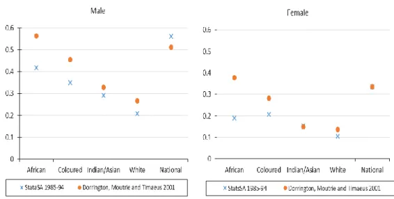
Figure 2.2: The probability of a 15 year old dying before reaching age 60 for different population groups in South Africa in 1985-94 and 2001. ... 24
Figure 2.3: The combined probability of a person aged 15 dying before reaching age 60 for both men and women in South Africa up-to 2015. ... 25
Figure 2.4: The level of 45q15 in the provinces among men and women in the years 1996 and 2001 ... 26
Figure 2.5: Prevalence of HIV/AIDS among antenatal attenders ... 27
Figure 2.6: HIV prevalence level among the districts in 2012. ... 28
Figure 4.1: Percentage of the 1996 population with unspecified population group ... 42
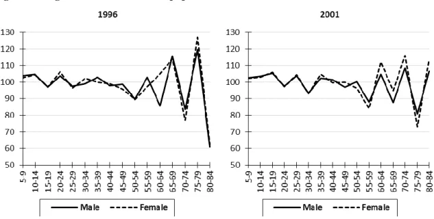
Figure 4.2: Sex ratios of population counts by age for the national and all population groups combined from the 1996 and 2001 census ... 43
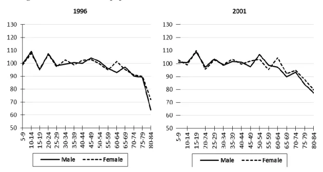
Figure 4.3: Age ratios for the African population in the 1996 and 2001 census ... 44
Figure 4.4: Age ratios for the White population in the 1996 and 2001 census ... 44
Figure 4.5: Age ratios for the Indian population in the 1996 and 2001 census ... 45
Figure 4.6: Age ratios for the Coloured population in the 1996 and 2001 census... 45
Figure 4.7: Proportions of African registered deaths by age for each sex ... 46
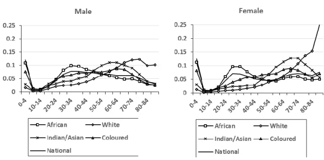
Figure 4.8: Proportion of registered deaths by age in the intercensal period 1996-2001 by population group ... 47
Figure 4.9: Proportion of household deaths by age reported in the 2001 census ... 48
Figure 4.10: Ratio of the proportion of household deaths to registered deaths in the year prior to the 2001 census, by population group. ... 49
Figure 4.11: Net numbers of migrants in the intercensal period between 1996 and 2001 .... 50
Figure 4.12: Proportions of the net numbers of migrants between the 1996 and 2001 census by population group ... 51
Figure 4.13: GGB diagnostic plots for completeness of registered deaths for the African population group ... 52
Figure 4.14: GGB diagnostic plots for completeness of registered deaths for White population group ... 52
Figure 4.15: GGB diagnostic plots for completeness of registered deaths for Indian population group ... 53
Figure 4.16: GGB diagnostic plots for completeness of registered deaths for Coloured population group ... 53
Figure 4.17: SEG diagnostic plots for completeness of registered deaths in the intercensal period ... 54
Figure 4.18: Ratio of the sum of expected deaths in the population groups to the number of deaths expected from the population as a whole by sex in the intercensal period 1996-2001 ... 56
Figure 4.19: Comparison of 45q15 derived from registered deaths after correcting for completeness with that derived from the orphanhood data for each population groups and each sex ... 58
Figure 4.20: Annual estimates of completeness for each population group and each sex over the intercensal period ... 58
Figure 4.21: Estimates of 45q15 for each year between the censuses of population groups by sex ... 59
Figure 4.22: Ratio of adjustment factors in the 2001 census by age for each population group and each sex ... 60
Figure 4.23: Estimates of 45q15 among men and women by district ... 64
Figure 4.24: Estimates of 45q15 for women against the HIV prevalence from antenatal women by district in 2001... 65
Figure 4.25: Comparison of provincial weighted average of district rates for 45q15from the households reported deaths against the provincial rates from the orphanhood method ... 67
Figure 5.1: Estimates of 45q15 obtained from this study compared against alternative
estimates from other authors and models in 2001 ... 71 Figure 5.2: Estimates of 45q15 for men and women in districts of South Africa ... 73
ACKNOWLEDGEMENTS
Firstly, I would want to thank God for his grace. I would also like to thank my wife and my son for their endurance and patience through the time of my studies. I also want to thank my supervisor Professor Rob Dorrington for his guidance and assistance
throughout the completion of this thesis. Last but not least, I would also want to thank the Andrew Mellon Foundation for funding my stay throughout the completion of my studies.
1 INTRODUCTION
1.1 Background
Adult mortality estimates are an essential component in guiding health policies and interventions. Since the start of the HIV epidemic in South Africa, over half of the deaths in the population have occurred in the adult ages from as early as 1999 (Statistics South Africa, 2005). Although it is important to understand the overall mortality in a nation, gaining a better understanding of the heterogeneity in mortality is of greater significance as it gives a better understanding when targeting specific areas for health intervention, allocating resources and setting priorities where mortality is high (Ahmed & Hill, 2011). At a sub-national level unhealthy districts and healthy districts can be used to generate debate about the general health in the country at the time (Mahapatra, Shibuya, Lopez et al., 2007). Sub-national estimates are essential in identifying the heterogeneity in the population, not just referring to the geographical location but also the population groups within the whole population. However, there is a debate about whether heterogeneity in the mortality of population groups is purely biological or due to social outcomes (Moultrie & Dorrington, 2012)? None the less it is certain that heterogeneity exists and should be accounted for. However, the required data for the measurement of sub-national level estimates are often not readily available, particularly in developing countries and the world’s poorest populations (Joubert, Rao, Bradshaw et al., 2012).
Although much progress has been made in estimating adult mortality at national levels in developing countries where the data are often incomplete or biased, no method currently exists that can be used to determine mortality accurately at a sub-national level (Ahmed & Hill, 2011). In most developing countries, death data used to obtain adult mortality estimates is sourced from the vital registration system and the census. The methods used to obtain mortality estimates can be either direct or indirect, depending on the nature of the data being used. Indirect approaches to estimating adult mortality nationally include the orphanhood and sibling history methods, whilst direct techniques include death distribution methods. However, use of these methods on a sub-national level is problematic for several reasons, most resulting from incomplete and missing information from the data sources.
There have been several attempts to produce provincial estimates of adult mortality (Statistics South Africa, 2000, Dorrington, Moultrie & Timæus, 2004,
Dorrington, Timæus, Moultrie et al., 2004, Msemburi, Pillay-van Wyk, Dorrington et al., 2014, Udjo & Lalthapersad-Pillay, 2014). The ASSA provincial demographic models also project the rates of adult mortality (Actuarial Society of South Africa, 2011). Among these, some studies (Udjo & Lalthapersad-Pillay, 2014, Dorrington, Timæus, Moultrie et al., 2004, Dorrington, Moultrie & Timæus, 2004, Dorrington & Timæus, 2015) have used a combination of vital registration and census data to come up with the provincial mortality rates.
Although the completeness of the vital registration deaths in South Africa has improved in the past two decades, vital registration still has some weaknesses that make it difficult to produce reliable estimates sub-nationally. As far as registered deaths are concerned there are three major concerns: coverage, completeness and missing data (Mahapatra, Shibuya, Lopez et al., 2007). Coverage is often higher in urban areas than rural areas, even in some areas where there is 100 per cent coverage, the data often contains missing information. Most if not all developing countries have incomplete death registration, but the completeness of registered deaths in South Africa has been improving over the last decade. Because ignoring unregistered deaths will lead to overstating life expectancy among other things, death distribution methods have been used to estimate and thus correct for incompleteness of death registration. However, one of the inherent weaknesses of vital registration data lies in its failure to locate the usual place of residence of the deceased, which is essential if mortality is to be measured at sub-national level.
On the other hand, data on deaths reported by households in the census are also problematic for different reasons, which include: recall bias, event omission, household collapse and inaccurate age reporting (Joubert, Rao, Bradshaw et al., 2012). Recall bias leads to deaths being reported for a longer or shorter period before the census than intended which results in under- (over-) reporting of deaths for a fixed period. Death omission may result from a household collapsing after the death of an individual which leads to under-reporting of deaths. Conversely, deaths of, for example, young adults who recently moved out of the household to look for work, may be reported by more than one household. Elderly households are prone to under-report deaths in the household as there may be no one to report the death. All of this could mean that completeness of deaths may differ by age.
Due to these errors it is more reasonable to assume that the reporting of registered deaths is more likely to be constant for all age groups above a certain
minimum age than the deaths reported by households are (Dorrington, Moultrie & Timæus, 2004), which is one of the major assumptions when applying death distribution methods. Dorrington and Timæus (Dorrington, Moultrie & Timæus, 2004, Dorrington & Timæus, 2015)have estimated provincial mortality in South Africa for 2001 and 2011 using the strengths in both sources of data to produce estimates of mortality at the provincial level. In a similar way, this study aims to assess the strength of the method at a district level.
1.2 Objectives of the research
This study mainly aims to assess the suitability of the adult mortality estimates obtained for each sex for the 52 municipal and metropolitan districts of South Africa in the year prior to the 2001 census by using the method of combining vital registration data and census data adopted from Dorrington, Moultrie and Timæus (2004).
However, in the process of producing the adult mortality estimates the following objectives must be satisfied.
1. Estimate national completeness of registered deaths for both sexes and also by population group for each sex in the intercensal period of 1996 to 2001. 2. Estimate completeness of registered deaths for each sex and population group
for the year prior to the 2001 census.
3. Estimate age-specific household correction factors for each sex and population group in the year prior to the 2001 census.
4. Estimate the true (corrected) deaths reported by households in each district by sex from the 2001 census.
5. Estimate district adult mortality rates by sex from the corrected reported deaths by households in the 2001 census.
6. Evaluate the suitability of the method in obtaining mortality estimates for 2001 at district level.
1.3 Significance of the research
The research enables us to examine the extension of the method proposed for provincial estimates by Dorrington, Moultrie and Timæus (2004) to the district level. Based on the outcome of the study, the method will either fail to produce convincing adult mortality estimates or produce reasonable estimates of adult mortality at the district level.
If the method fails to produce reasonable estimates of adult mortality at district level, it is essential that the weaknesses in applying the method are discovered from this study for the benefit of future studies using a similar approach. A cross examination of the methodology and the data will guide future studies in addressing the methodology changes and (or) fundamental data needs that may ensure more reasonable estimates of adult mortality at the district level.
On the other hand, if the method is found suitable its will enable us to make use of the method elsewhere. Estimates of adult mortality at the district level will help inform health policies. The estimates may be used as a guide for improving health delivery at sub-national level in an effort to reduce the burden of adult mortality, specifically targeting diseases with a high prevalence in adults that lead to early death such as HIV/AIDS.
1.4 Structure of the research
The dissertation consists of five chapters. Chapter two reviews the sources of mortality data, death distribution methods, the level and trend of mortality in South Africa and reviews studies that obtained mortality estimates using a combination of vital
registration and census data. In Chapter 3 the method used specifically in this
dissertation is presented. Chapter 4 presents the results obtained from implementing the method. The last chapter reflects on the results and discusses the extent to which the district adult mortality estimates are accurate.
2 LITERATURE REVIEW
This chapter generally seeks to understand the limitations and strengths of tools
designed to produce estimates of adult mortality at the sub-national level. It also aims to understand the efforts made by different studies in the area of estimating mortality at the sub-national level. The chapter begins by reviewing the potential sources of
mortality data. In the same section we consider the extent to which the different sources of data are useful to estimating mortality at the sub-national level.
Thereafter the chapter reviews several methods that have been proposed for estimating adult mortality. This starts with a review of the death distribution methods in depth by looking at its foundation and establishing the requirements essential to
obtaining reliable estimates. This is followed by a review of the orphanhood method. In the last part of this section studies that have produced estimates of provincial adult mortality are reviewed.
The final section of the chapter covers estimates of the level and trends of adult mortality to understand the general trajectory of mortality up until 2001. In particular it covers the level of mortality for different population groups and provinces from various studies and the level of HIV prevalence at the sub-national level.
2.1 Sources of mortality data
In developing countries, the sources of data necessary for estimating mortality rates are usually obtained from vital registration, censuses, surveys and surveillance sites. The validity of any of the estimates produced will depend on the data quality. However, in most developing countries these different sources have problems which limit their usefulness in producing accurate mortality estimates.
Household surveys such as the Demographic Health Survey (DHS) have been used extensively in estimating mortality in developing countries, particularly of child mortality. Questions relating to sibling and parental survival are used in the indirect estimation of adult mortality. Survey data relating to child mortality has, generally, produced better estimates compared to adult mortality (Timæus, Dorrington & Hill, 2013). This is because unlike child deaths, adult deaths are not concentrated in a narrow age group, thus bias in results is greater in estimating adult mortality. Apart from that, data relating to adult deaths are not specific to a unique respondent; questions relating to orphanhood and sibling survival may be answered by multiple individuals referring to
a single death, unlike the mother in the case of a child death. Adult deaths, thus, may be over-reported or under-reported. Although data quality can be monitored, survey death data are not appropriate for estimating mortality sub-nationally because the sampling procedure in identifying households for the survey is taken to be nationally
representative, which may not be representative of the sub-national units. Generally in South Africa, the use of surveys in adult mortality estimation has been limited. During the late 1990s the October Household Survey (OHS) was used in the estimation of mortality as there were a few sources to rely on at the time (Udjo, 2016).
Small area systems such as the Health and Demographic Surveillance System (HDSS) sites have been useful over the past decade in monitoring demographic events. They ensure platforms for further research into cause-specific mortality, for example, maternal mortality and HIV/AIDS; however, they represent a small geographical area, which is usually not representative of the national population (World Health
Organisation, 2006). Nonetheless they are useful in building an understanding of how different socio-economic and health outcomes will lead to different levels of mortality. Furthermore HDSS can be used for investigating causal factors of mortality, which may be difficult to identify using other sources of death data.
Deaths recorded in hospitals can also be a useful source of data, particularly when assessing the causes of death. In some countries, like Botswana where it is said that more than 90 per cent of the deaths occur in health facilities (Negussie, Will, Bodika et al., 2009), this source of death data can be a substitute for registered deaths and may also provide information about causes of death. However, for most developing countries, a significant number of deaths occur outside health facilities. Most of these deaths occur particularly in the rural areas resulting in an uneven death coverage of the population. In addition to the low coverage of deaths in hospitals, the deaths may be selective according to the causes of death, which results in the clustering of certain causes of death in the hospitals more than other causes. Recorded deaths from hospitals are likely to be selective of the location, in other words, deaths will likely end up in the nearest hospital which may even be outside the district of residence. In addition, data on hospital deaths are not easy to access as the databases for the different hospitals are not openly accessible and often not updated regularly (Khoza, 2009).
Registered deaths are the best source of mortality data for comprehensive and continuous monitoring of public health programmes over time (Mahapatra, Shibuya, Lopez et al., 2007, Mathers & Boerma, 2010), yet, only 30 per cent of the world live in
areas where registration is more than 90 per cent complete (Joubert, Rao, Bradshaw et al., 2012). In South Africa, it is a legal requirement for all people to register a death once it has occurred. If the death occurred in a hospital, a family member or the funeral undertaker can report it to the nearest local Home Affairs office, otherwise, if it occurred elsewhere, either the family member or funeral undertaker registers the death with the local municipality as well as the municipal Home Affairs office for acquisition of burial space (Khoza, 2015). The population register is also updated at the local Department of Home Affairs (DHA), taking account of the deaths that have a South African identity number from the South African-born population. Thereafter, the death notification forms are sent to Stats SA for the production of vital statistics (Khoza, 2015).
The framework proposed by Mahapatra, Shibuya and Lopez et al. (2007) for assessing the quality of general vital registration data is to assess the accuracy, relevance, comparability, timeliness and accessibility of the data. The timeliness of vital
registration data in South Africa has improved considerably since 2004. One of the reasons for the reduction in time to release mortality data is faster processing of the death notification forms by Stats SA (Khoza, 2015). The delay in releasing deaths data has reduced to a lag of 11 months from a lag of seven years in 2003. The accuracy of the vital registration deaths is also affected by coverage issues, which hinder registration as the DHA may not be easily accessible in some areas. Urban areas are more likely to have higher coverage than rural areas. Another problem that affects the quality of death registration data is variables with missing responses, especially on key variables such as gender and age, which will affect the usefulness of the data. For example, a small proportion of death notification forms lose either the first or second page when the death notification forms are transferred to Stats SA (Khoza, 2015).
Death notification forms now include the usual place of residence of the deceased as well as the place where the death occurred (Statistics South Africa, 2014), whereas previously registered deaths recorded only the place of occurrence, which probably concentrated deaths at health facilities (Dorrington, Moultrie & Timæus, 2004). In many developing countries, the time it takes for the data to be published and the ease of access are also a concern. However, in South Africa, Stats SA releases reports periodically on their findings from captured mortality data from the vital registration deaths.
Despite the errors in vital registration data, the major concern, that of
incompleteness of registration, can be corrected for adult ages using death distribution methods. Although deaths are liable to late registration, the date on which the death occurred is accurately recorded, implying the correspondence of deaths to the
population in estimating mortality is relatively accurate for those deaths that have been reported.
Unlike registered deaths, data on deaths reported by households are not collected continuously as they depend on the census having taken place, usually every ten years. Census data for South Africa currently incorporates questions involving the survival of parents as well as deaths reported by households in the last year. South Africa has had three post-apartheid censuses, namely in 1996, 2001 and 2011, although the 1996 census did not include the question on deaths reported by households in the last year. Deaths reported by households (HHD) rely on the respondents accurately recalling the death of household members in the year before the census.
One of the strengths of HHD over registered deaths is that they are reported according to the usual place of residence, which is useful in obtaining sub-national estimates of mortality directly. However, one of the concerns with HHDs is reference period error, where deaths which occurred outside the reference period are reported as occurring in the period and vice-versa, thus leading to over- (under-) reporting of deaths, which affects the quality of estimates (Mathers & Boerma, 2010).
Not every death is of a person living in a household, that is to say HHDs may not constitute full coverage in the population, for example, deaths occurring in retirement homes are not included under HHDs, which is apparent in the White population (Dorrington, 2013c). However, in the 2011 census, Stats SA report that converted hostels were included in the final reported deaths (Statistics South Africa, 2012a, p.68), although their definition is not clear on the difference between institutions and converted hostels (Statistics South Africa, 2012b). In addition, some deaths in the household may be missed, for example, households dissolving when a key member has died, which leads to under-reporting of deaths. More so for small and young families at the time when HIV was at the peak before the introduction ARVs (anti-retrovirals): they would then have a greater risk of both infected parents dying, leaving the household isolated or with young orphans who may be taken into orphanages or fostered.
Another weakness of HHDs can arise from multiple reporting of deaths. Young adult deaths may be reported by more than one household due to the young adults
having dual residences, which may be caused by migrating elsewhere in search for employment. Also the age at death of a household member may be misreported, particularly at older ages where it may be exaggerated (Dorrington, 2013b).
Nonetheless, census data is easily accessible. Most of the census data are openly available from the Stats SA interactive data websites; Nesstar and SuperWeb, and variables not available may be provided upon request to Stats SA.
2.2 Methods of estimating adult mortality
2.2.1 Death Distribution methods
Death distribution methods are used to estimate the completeness of death reporting in the population, which essentially allows one to correct for the incompleteness of death reporting in producing estimates of mortality. The principle behind death distribution methods were developed by Brass (1975) and Preston, Coale and Trussell et al (1980). Originally, these methods compared deaths with population counts at a single point in time on the assumption that the populations are stable. However, they were later generalised to make use of two censuses and thus to be of more practical use for populations which are not stable.
There are two approaches: the General Growth Balance (GGB) method and the Synthetic Extinct Generations (SEG) method. Both of these, however, require certain assumptions about the data to be satisfied. These assumptions are: that there is a constant under- (over-) count in all age groups in each of the censuses; that the population is closed to migration; that completeness of reporting of deaths is constant (at least for adult ages); and that the ages of the living and the deceased are reported to be reasonably accurate (Hill & Queiroz, 2010). Although both methods use the same data, in some instances they produce different results due to the nature of data errors and violation of assumptions. One could also consider the method of initially applying the GGB method to estimate the parameter δ to be used in the SEG method on the same input data to estimate completeness, which is referred to as GGB-SEG
throughout this dissertation. 2.2.1.1 General Growth Balance Method
The GGB method was generalised from the Brass Growth Balance (BGB) by Hill (1987). The BGB was proposed by Brass on the basis that it is possible to estimate the completeness of reporting of deaths if population counts are available from a single
census provided the population is stable. The GGB method is derived from the population balance equation assuming the population is closed to migration:
2 , 1 2 , 1 1 2
P
B
D
P
where Pi is the total population at time of census i, also
B
1,2 andD
1,2 are the totalbirths and deaths respectively in the intercensal period. This equation can be generalised to the open age interval (aged
a
and older) to give:)
(
)
(
)
(
)
(
1 1,2 1,2 2a
P
a
B
a
D
a
P
Dividing the entire equation by the total person-years of exposure, which is
approximated by the geometric average population in the open age interval (
a
) at the start and end of the intercensal period multiplied by the length of the interval,
0.52 1
(
a
)
P
(
a
)
P
t
, and dropping the time of the census for convenience:) ( ) ( ) (a b a d a r (2.1)
where: r(a) is the true growth rate of the population; b(a) is the true rate at which
the population turns
a
and older; d(a)is the true death rate of the population in theopen age interval.
The BGB uses a constant growth rate since it assumes the population is stable. The GGB, on the other hand, tries to account for the violation of that assumption in reality by making use of two census counts to estimate the age-group specific growth rates in the open age interval. However, since the censuses are prone to under- (over-) count and deaths are liable to under- (over-) reporting relative to the second census, the observed census counts can be expressed as P1 (a)
o and
) (
2 a
Po , and the reported deaths as D(a). The observed and true values are related as follows:
) ( 1 ) ( P a k a P io i i ) ( 1 ) ( D a c a D o
where: ki is the proportion counted from census i;
c
is the proportion of deaths registered in the intercensal period reported.In estimating the total population turning
a
in the intercensal period, B(a),where
N
k(
i
,
j
)
is the population aged between i and j in census k, under theassumption that there is constant under- (over-) count in all age groups, substitution results in
1
( ) ) 5 , ( 1 ) , 5 ( 1 5 ) 5 , ( ) , 5 ( 5 ) ( 0.5 2 1 5 . 0 2 2 1 1 5 . 0 2 1 B a k k a a N k a a N k t a a N a a N t a B o o oAlso substituting for total person-years of exposure in the intercensal period gives:
0.5
2 1 5 . 0 2 1 5 . 0 2 1 ( ) ( ) 1 ) ( ) ( t P a P a k k a P a P t o oSubstituting the above equations into each component of the population balance equation gives: ) ( ln 1 ) ( ) ( ln 1 ) ( 2 1 1 2 r a k k t a P a P t a r o (2.2)
( ) ) ( ) ( ) ( ) ( ) ( ) ( ) ( 0.5 2 1 5 . 0 2 1 5 . 0 2 1 5 . 0 2 1 a b a P a P t k k a B k k a P a P t a B a b o o o o
( ) ( )
( ) ) ( ) ( ) ( ) ( ) ( 5 . 0 2 1 5 . 0 2 1 5 . 0 2 1 5 . 0 2 1 d a c k k a P a P t a D c k k a P a P t a D a d o o o oThe growth rate is estimated differently in equation 2.1 and equation 2.2 given equation 2.1 assumes a linear growth, whereas equation 2.2 assumes an exponential growth, although the difference is insignificant for small values of the growth rate for the open age interval (Hill, 1987). Substituting the equations above into the balancing equation gives:
) ( ) ( ln 1 ) ( 5 . 0 2 1 2 1 d a c k k a b k k t a ro o o
) ( ln 1 ) ( ) ( 5 . 0 2 1 2 1 d a c k k k k t a r a bo o oA straight line can be fitted to the data points with bo(a)ro(a) on the y
-axis and the observed death rate in the open age interval on the
x
-axis, and an intercept of ln
k1 k2
t and a slope of
k
1k
2 0.5c
. Once the estimates of the slope andintercept are obtained, values of the census under- (over-) count and under- (over-) reporting of deaths can be obtained. However, since there are two equations and three unknowns, the equation can only be solved with two unknowns. This is done by expressing the under- (over-) count of one population relative to the other, that is one of the k’s is usually assumed to be the lower of the two with the other taking a value of
unity, which is appropriate since there is usually no ideal census with the true count. Although there are many methods that can be used in fitting the straight line, such as
the method of least squares, orthogonal regression, grouped mean and weighted means, the method of least squares and un-weighted methods are not recommended for fitting the line as they give too much weight to extreme data points (Bhat, 2002, United Nations Population Division, 2002, Marandu, 2011). Orthogonal regression to fit the straight line is recommended (Bhat, 2002, Dorrington, 2013b) since it produces a better fit in cases where age exaggeration exists, which is typical of data in developing
countries, more so at the older ages. 2.2.1.2 Synthetic Extinct Generations method
The SEG method proposed by Bennett and Horiuchi (1981, 1984) is a generalisation of the method proposed by Preston et al. (1980) which was itself an extension of the method of extinct generations proposed by Vincent (1951). The method of extinct generations uses the idea that the population at any age and at any point in time can be estimated from the future deaths from that cohort until the last individual dies, which can be expressed as follows:
dx x t D t Na( ) a x( ) 0
(2.3) where; Na(t) is the true population ageda
last birthday at timet
; Dax(tx) are the true deaths in the yeart
x
ageda
x
last birthday; ω is the age of the last death in the cohort. However, applying this method would require one to wait for the cohort to die out. Additionally this method requires deaths data to be collected on the same cohort over time, which may be problematic due to migration and lack of follow-up. This would be simpler if the population is stationary, as the number of deaths at each age remains constant over time, although this is not so in reality.Preston, Coale, Trussell and Weinstein (1980) generalised the method for
populations that are close to being stable so that one uses the current numbers of deaths by age to estimate the future deaths in the population since the deaths at each age change by a constant rate each year over time. That is,
rx t D x t Dax( ) a( )exp where ris the annual growth rate of the population.
However, most developing countries have populations that deviate from stability. Thus Bennett and Horiuchi (1981, 1984) further generalised the method
proposed by Preston et al. (1980) to non-stable populations by using age-specific growth rates estimated over an intercensal period to estimate future deaths:
x a i a x a t x D t rdi D ( ) ( )expwhere ri is the growth rate for age i.
The method of synthetic extinct generations as proposed by Bennett and Horiuchi uses the assumption that the current growth rates in the intercensal period apply in the future. However, one is not necessarily restricted to this assumption as it can be shown that the current population can be expressed in terms of the current deaths and the current growth rates in the intercensal period (Dorrington, 2013c, Preston, Heuveline & Guillot, 2001, p171-172):
dx di r t D t N a x a i x a
( )exp ) (Bennett and Horiuchi (1981, p221) propose the following approximation to the above equation to apply to five-year age groups:
a a
a
a
a
t
N
r
D
r
N
(
)
5exp
5
5
5exp
2
.
5
5To take into account the under- (over-) reporting of deaths, let the observed deaths between age
a
and a5 be represented by 5D
ao and the completeness of reported deaths bec
. This means that the product of true deaths andc
gives the reported deaths, and this adjustment can be allowed for in the above equation which can be shown to be:
a
o a a a a t N r D r Nˆ ( ) ˆ 5exp 55 5 exp 2.55 (2.4) However, since the equation is applied iteratively from the open age interval to lower ages, Bennett and Horiuchi (1981) also proposed a way to estimate the population at the open age interval, A. Apart from using the deaths in the open age interval one needs the life expectancy in the open age interval (eA) to account for the variation in the age at death above A, more so when the open interval is set to be relatively low:
6 exp ˆ A A 2 A A o A A e r e r D N The estimate of life expectancy at the age of the open interval can be obtained using several methods. One could estimate it based on independent estimates from other research on the same population. An alternative would be applying the GGB method to
the same data to derive a life table and hence estimate life expectancy at age A. One could also use the ratio of reported deaths, 30
D
10o 20D
40o , and compare it to an equivalent level in the Coale and Demeny model life tables, but this may not give suitable estimates in populations affected significantly with HIV/AIDS as the Coale and Demeny model life tables do not reflect AIDS mortality (Dorrington, 2013c).Alternatively, one may also start with an initial guess of the life expectancy and obtain the results from the SEG, and thereafter use the results to construct a life table, then iterate to a solution (Dorrington, 2013c). The significance of the error in estimating life expectancy decreases the higher the age of the interval (Bennett & Horiuchi, 1981).
Once the number of people in the population in the age groups have been estimated from the deaths, the annual average population in the intercensal period in each of the five-year age groups (5Nˆa) can then be estimated:
5
5 ˆ ˆ 5 . 2 ˆ a a a N N t NThe annual average population estimated from the numbers counted in the two censuses in the intercensal period is:
2
0.5 5 1 55Na Na Na
where 5
N
ai represents the population in census i aged betweena
and a5. Therefore, completeness of reporting deaths can be estimated by the ratio of the cumulated population obtained from the observed deaths and the age distribution from both censuses assuming the level of death reporting is constant over the cumulated age groups: a a A a a A N N c ˆThe completeness of death reporting is not determined in the open age interval as this interval is more sensitive to the error in estimating the life expectancy, eA. One may also consider changing the open interval A to lower ages if there is evidence of significant age exaggeration at the older ages (greater than 60), which can be noticed by comparing visually the data points
a
against the starting agea
of each age interval to a trend line. A gradually consistent decrease in completeness at the older ages would indicate age exaggeration.Since the censuses may be under- (over-) counted, the growth rates used in obtaining equation 2.4 should be adjusted to take this into account. This adjustment was
previously derived in the review of the GGB as ln
k1 k2
t, is referred to as δ byBennett and Horiuchi (Dorrington, 2013c), and can be estimated iteratively by adding different values of δ to the observed growth rates until the plot of
a
against the starting agea
of each age interval reflects the most level set of ratios (Dorrington, 2013c). When this adjustment is applied, we refer to the method as the SEG+δ, otherwise the SEG. 2.2.1.3 Problems of using Death Distribution Methods with registered deathsFor the errors that the methods were developed to overcome, the methods are reported to perform particularly well by researchers who have looked at DDMs response to various errors (Hill, 1987, Hill, You & Choi, 2009, Dorrington, Timæus & Moultrie, 2008). These errors include omission of deaths, changes in census coverage and omission of deaths occurring together with a change in census coverage (Hill, You & Choi, 2009).
Research (Dorrington, Timæus & Moultrie, 2008, Hill, You & Choi, 2009) suggests that if migration in the population is significant and has not been accounted for, the error in the estimate of completeness is higher than most of the typical errors one may encounter. However, it is suggested (Dorrington, 2013b, Murray, Rajaratnam, Marcus et al., 2010) that if the points used to fit the straight line to determine
completeness for the GGB indicate migration effects1 it may be useful to confine the fit to higher ages where the fit seems to be consistent with the straight line to help
eliminate potential migration effects, although there are concerns that it may increase the possibility of error in estimating the completeness due to age exaggeration at older ages (Hill, You & Choi, 2009). Hill and colleagues suggest that when emigration is unaccounted for and there is an error in estimating increasing census coverage, the SEG method performs particularly better than the rest of the methods.
The percentage errors in the estimate of 45q15was higher than that for 25q60 in the GGB, SEG and GGB-SEG methods when completeness was either increasing or decreasing with age (Hill, You & Choi, 2009), this may also support the indication of using a narrower age interval in estimating completeness.
International migration is quite difficult to account for accurately in most countries. Immigrants may not be willing to answer questions on the census because of the fear of their illegal status in the country and also the fear of xenophobia, resulting in
1
Migration effects in the fitted straight line can be noticed by deviation from the straight line at ages usually lower than 35 since much of the migration in a population is usually concentrated around these ages unless the context of the population suggests otherwise.
the net migration likely being under-represented (Dorrington & Hill, 2013). Emigration, on the other hand, is even more difficult to account for as it requires the combination of information from receiving countries in their census which may not correspond with the census date being used (Dorrington & Hill, 2013).
Stats SA’s assumptions for the population projections used to produce mid-year population estimates (Statistics South Africa, 2015) were that generally, the African and Indian2 population groups experience immigration, with the White population
experiencing significant emigration (Dorrington, Moultrie & Timæus, 2004), and the Coloured experiencing negligible net migration. Khoza (2015), using the DDMs, assumes a zero net migration between 1996 to 2001 and 2001 to 2006; however, between 2001 to 2006 the results seem to suggest unaccounted for migration, although Khoza is open to the possibility that the effect may be due to the use of the 2007 Community Survey rather than an actual census.
At the national level net-migration is less volatile and less significant compared to the sub-national level. For this reason DDM’s are increasingly less reliable due to migration effects at the sub-national level. The method of combining the vital registration and HHD proposed by Dorrington and Timæus was proposed as a way
around having to measure completeness at the sub-national level. Dorrington, Moultrie and Timæus (2004) estimated the completeness of death
registration in each of the population groups in the intercensal period 1996-2001 using the GGB. Migration in other population groups except for the White population is identified to be insignificant. However, emigration is estimated using the censuses from the main recipient countries of the South African-born White population. In spite of the effort to estimate net migration the results for the White population appeared
implausible. The need to allow for migration in applying DDMs restricts their use as there is need to accurately estimate net migration.
Age exaggeration at old ages is common, which results in bias in the estimates of overall completeness. When using the GGB method to estimate completeness, age exaggeration can be noticed from the diagnostic plots by points at the older ages deviating from the fitted straight line; likewise by an inconsistent rise and drop in the completeness at the older ages in the SEG and SEG+δ methods (Dorrington, 2013b).
2
Generally, the GGB method performs better where there is age exaggeration than does the SEG and SEG+δ methods (Dorrington, 2013b, Hill, You & Choi, 2009).
Murray, Rajaratnam and Marcus (2010) suggest there is evidence of significant variation in the age ranges that produce the best results when comparing the DDMs. In their research, the ideal age range for the GGB, SEG and GGB-SEG methods is 40 to 70, 55 to 80 and 50 to 70 respectively. In addition, the SEG reflected a consistent pattern of error reduction with older age ranges as opposed to the other methods. Although not specified it may be that SEG+δ follows the same behaviour3.
Furthermore, when patterns of age misreporting differ widely between the two censuses and registered deaths, the error increases in the GGB, SEG and GGB-SEG methods (Murray, Rajaratnam, Marcus et al., 2010).
It is worth mentioning that the data used in both studies (Hill, You & Choi, 2009, Murray, Rajaratnam, Marcus et al., 2010) did not take into account the impact of HIV/AIDS unlike Dorrington, Timæus and Moultrie (2008), thus some of the results may possibly not be generalisable to the South African context. In addition Murray, Rajaratnam and Marcus et al. (2010) used a different age pattern for migration in their scenarios, and some of the statistical assumptions underlying their modelling are not clear enough to allow replication of the full scenarios.
Both Hill, You and Choi (2009) and Dorrington, Moultrie and Timæus (2008) seem to agree that the SEG performs better in errors combining emigration and increasing census coverage. However, the authors’ conclusions seem to differ as Hill, You and Choi (2009) conclude that GGB-SEG is the best method with an age range of 5+ to 65+ and Dorrington et al. (2008) concludes SEG+δ performs better in most of the scenarios on average than the GGB and GGB-SEG. However, results in
Dorrington, Moultrie and Timæus (2004) are strengthened as the methods are applied to typical African population data in the context of South Africa with the HIV/AIDS epidemic.
2.2.2 The Orphanhood method
The orphanhood method uses questions on the survival status of parents to estimate adult mortality. One of the advantages of this method is that the questions are simple to answer and eliminate recall bias by not requiring recall of either the date or the age when the death occurred.
3
Since the two methods follow the same general approach in terms of the general methodology, it may be that the SEG and SEG+δ both respond better to older age ranges.
The method uses the age of the respondent and the mean age of childbearing of the mother4 (conception for the father) in estimating the exposure to the risk of dying of the parents through the probability of the parents’ survival from that age to the time of the survey. Conditional survivorship of the parent is estimated as the probability of the mother of the respondent having had survived from the mean age of child bearing to the age of the respondent (lmn lm, where m is the mean age of childbearing and n is the age of the respondent). To obtain the estimate of this conditional probability a
regression equation making use of the proportion of respondents in a particular age group with living mothers and coefficients of survivorship for women (men) is used (Timæus, 1992). Thus, the older the respondent is, for example, the longer the parent has survived.
Since the conditional survivorship refers to different probabilities of survival as well as different mortality experiences, it becomes necessary to standardise the
conditional survivorship into one measure that can be comparable through time, for example, 35p25, the probability of a person aged 25 dying before reaching age 60. The conditional survivorship in each age group is standardised using the two parameter relational logit model, which connects the estimated mortality experience to that of any standard life table (Murray, Ferguson, Lopez et al., 2003, p.166-168). In application (Timæus, 2013), the age pattern of mortality is determined by a life table that reflects the same age pattern of mortality as the population on which we seek to estimate mortality5. The time location of the estimate from the time of the census depends on the level of mortality and can be estimated from the proportion of surviving parents, the age of the respondents and the mean age at childbearing of the parents (Timæus, 2013).
However, this method usually produces more reasonable estimates using
responses from female respondents rather than male respondents, as women are usually closer to their parents than men. In addition, the method produces some bias in
mortality estimates as those parents without surviving children are not represented whereas those with more than one surviving child may be over-represented; however, the bias in the final estimates is small, except in populations affected by HIV/AIDS, especially before ARVs were accessible, due to infected adults dying before their parents
4
The mean age at childbearing is calculated from the census information by dividing the age-weighted sum of births by the total number of births. The mean age of conception for the father is calculated by adding the difference between the median age of marriage for men and that of women.
5
Moultrie Tom A & Ian M Timæus 2013. Introduction to model life tables. In: Moultrie, T., Dorrington, R., Hill, A., Hill, K., Timæus, I. & Zaba, B. (eds.) Tools for Demographic Estimation. Paris: International Union for the Scientific Study of Population: Available: http://demographicestimation.iussp.org/content/introduction-model-life-tables.
since they will no longer be able to report the survival status of their parents (Timæus, 2013). The adoption effect also presents a problem at younger ages where children may report their parents as surviving when in fact they are deceased but due to the nature of their adoption they may consider their guardian as the parent. However, Timæus (2013) tries to reduce this bias by using respondents aged 20 onwards, since the bias is likely to be greater when the respondent is still young. Although it is possible to apply the orphanhood method sub-nationally, one should do so with caution in the knowledge that parents do not always live in the same area as their children and thus the mortality experience may not be consistent with the location.
2.3 Estimating mortality sub-nationally
Sub-national mortality estimates are quite problematic to produce accurately if the data is prone to errors and bias. However, in South Africa there is growing research in the area as the accuracy of data sources continues to improve. Usually when one thinks of estimating completeness of reporting deaths, death distribution methods are used, although as pointed out earlier, these methods cannot be applied at a sub-national level. The reason being compared to international migration, inter-provincial migration is more dominant and difficult to measure or estimate accurately, which is one of the requirements when applying death distribution methods (Dorrington, 2013b).
Dorrington and colleagues (Dorrington, Timæus, Moultrie et al., 2004) in producing provincial estimates of mortality from the vital registration deaths for 1996 linked completeness of registered deaths for children to that of adults, assuming a linear relationship between the two. The relationship was established on the assumption that the mortality rate of adults between 65 and 70 (5m65) did not differ significantly between the provinces at the time, thus any difference between the provinces can be attributed to the completeness of death registration. Although there is no justification for the linear relationship between completeness in adults and that of children, a weak correlation for both sexes between child completeness and mortality for older ages was obtained (Dorrington, Timæus, Moultrie et al., 2004).
The results for completeness indicated high levels of death registration in Gauteng, Northern Cape, Western Cape, North West and Free State (118%, 118%, 117%, 107% and 105%), and low levels of registration in Eastern Cape, Limpopo and Mpumalanga (57%, 60% and 85%). It is suggested that the completeness of reporting of deaths in some provinces appeared implausible, namely, the high levels in completeness in Free State and North West could possibly be due to the poor coverage in the census
rather than registration of deaths from other provinces. However, the post-enumeration survey results reflect the highest undercount in Northern Cape, Kwa-Zulu-Natal and Limpopo (15.59%, 12.81% and 11.28%), with the lowest in Western Cape, Free State and North West (8.69%, 8.75% and 9.37%) (Statistics South Africa, 1998). This conflict in results was not interrogated further.
One of the limitations of this study is that the questions relating to deaths in the household were not asked in the 1996 census. So for subsequent censuses Dorrington and colleagues (Dorrington, Moultrie & Timæus, 2004, Dorrington & Timæus, 2015) used a different approach, which we seek to adopt in this study, in their estimation of provincial mortality estimates in 2001 and 2011. Unlike the prior study (Dorrington, Timæus, Moultrie et al., 2004), deaths reported by households are scaled using the results of completeness from registered deaths.
Generally, the studies (Dorrington, Moultrie & Timæus, 2004, Dorrington & Timæus, 2015, Pillay-Van Wyk, Laubscher, Msemburi et al., 2014) apply the DDMs initially to the registered deaths in the intercensal periods in estimating overall national completeness of death registration for each sex and each population group.
Completeness was higher for the White population, followed by the Indian, Coloured and least in the African population, with females having higher values of completeness than males, possibly due to the fact that women are not as mobile as men and therefore less difficult to track than men (Dorrington, Moultrie & Timæus, 2004). Interestingly, the difference between the completeness of Indian men and women was quite large.
After this the completeness of death registration in the year preceding the census is estimated by fitting a trend to estimates of completeness obtained from using previous intercensal periods, since DDMs estimate the average completeness in the intercensal period and not the year before the census. The trend in completeness is fitted using a regression curve, which follows a known pattern of how completeness has been changing over time, for example, the logistic curve (Dorrington & Timæus, 2015, Pillay-Van Wyk, Laubscher, Msemburi et al., 2014). Alternatively, one could fit a trend to annual estimates of an indicator of mortality, for example, using m65from which the trend in completeness could be implied (Dorrington, Moultrie & Timæus, 2004,
Dorrington, Timæus, Moultrie et al., 2004). In obtaining the trend in completeness from 2001 to 2010, a logistic trend was fitted to the completeness in the period 2001 to 2007 after applying DDMs to the intercensal period (Pillay-Van Wyk, Laubscher, Msemburi et al., 2014). The trend was assumed to reach an asymptote of 93 per cent by 2009 as no
data was yet available at the time for 2011 registered deaths. However, the trend was verified for consistency by applying the DDMs to the intercensal period 2001-2011 using the estimate of registered deaths from the national population register for 2011 where registered deaths were not available (Dorrington, Bradshaw, Laubscher et al., 2015).
Once completeness is estimated in the year preceding the census, it is applied to estimate the true registered deaths for each sex, population group and the entire
population (Dorrington & Timæus, 2015). However, the sum of the deaths corrected for completeness by population group are adjusted to match the national deaths corrected for completeness. This is done to ensure consistency in the true national deaths including those that were not reported since realistically it is expected that the national deaths are sub-grouped into the four population groups.
The deaths reported by households from the census are then divided by the true reported deaths to estimate adjustment factors for each sex, population group and age-groups. These adjustment factors indicate the under- (over-) reporting of deaths by households. The deaths reported by households in each province according to sex, population group and age-group are multiplied by these adjustment factors. However, the adjustment factors assume that there is no significant difference in the under-(over-) reporting of deaths by households in each of the provinces. The true deaths reported by households in each province are then divided by the estimate of the population to produce crude estimate of the mortality rates.
After estimating 50q15 for each of the provinces using the deaths reported by households, the results were compared to corresponding results from the orphanhood. The results showed a strong correlation, indicating consistency between the two different estimates (Dorrington, Moultrie & Timæus, 2004).
2.4 Levels and trends of adult mortality in South Africa
2.4.1 The national level and trend of adult mortality
A lot of uncertainty lies in the mortality estimates for the period 1983-93. During this period the usefulness of censuses or surveys from which mortality estimates could be obtained was limited. Another reason for the uncertainty in estimates is the fact that death registration in South Africa did not include the so-called TBVC (Transkei, Bophutswana, Venda and Ciskei) areas. The TBVC areas under the apartheid government were designated as self-governing countries and specifically for the
of deaths was done independently in each of these areas, although these areas were unable to carry out death registration. Because about 25 per cent of the total African population in South Africa resided in these areas it may be possible that the level of mortality estimated in the period excluding these areas could have under-estimated the true level of mortality. Also the official South African life tables for 1984-86 were not representative of the black African population (Dorrington, Bradshaw & Wegner, 1999). However, Dorrington, Bradshaw and Wegner (1999) estimated the mortality of the African population in order to produce a nationally representative life table. This was done by averaging the mortality estimates from two scenarios, namely, estimating the mortality of the African population on the assumption that all TBVC deaths were reported in South Africa and on the assumption that the mortality in TBVC areas reflected an equivalent mortality rate as that of Africans in South Africa6.
From the late 1980s to the mid-1990s, adult mortality appears to have been constant to slightly decreasing, although the estimates from different authors vary on the extent of the decrease (Udjo, 2001, Dorrington, Moultrie & Timæus, 2004), as evidenced from most of the estimates in Figure 2.1 except for the indirect estimates obtained from the Demographic and Health Survey (DHS) in 1998. In 1985, the probability of a person aged 15 dying before age 60 (45
q
15) nationally for males andfemales was 38.4 and 25.4 per cent respectively (Bradshaw, Dorrington & Sitas, 1992), we expect the level of adult mortality 15 years later to be higher due to better
completeness of recording deaths and also the contribution of the HIV epidemic that followed during the period.
6
The first scenario estimates mortality using the total population of South Africa (including TBVC areas) and the deaths reported in South Africa, whereas the second scenario used the South African population excluding the TBVC.
Figure 2.1: The probability of a person aged 15 dying before reaching the age of 50 for South Africa up-to 2001.
Source: Figure 6.1; page 65; Dorrington, Moultrie and Timæus (2004)
Notes: VR stands for vital registration deaths, DHS for Demographic Health Survey, OHS for October Household Survey and DMT for Dorrington, Moultrie and Timæus.
Udjo and colleagues (Udjo, 2016, 2001) also argue that female mortality in the period 1980-1990 generally declined for all population groups, with Africans having the highest mortality and the White population having the lowest mortality. Stats SA (2000)
estimates from the 1985-94 abridged life table suggest a consistent ranking in the adult mortality for males with Africans having the highest mortality, followed by the
Coloured, Indian/Asian and then the White population in that order; however, somewhat strangely, a different ranking is estimated for the female population. A slightly higher estimate was obtained for the Coloured population than the African population7.
7
The probability of a person aged 15 dying before age 60 for African females in 1985-1994 is estimated to be 19.1 deaths per 100 individuals, whereas that for the female coloured population is estimated to be 20.5 deaths per 100 individuals.
Figure 2.2: The probability of a 15 year old dying before reaching age 60 for different population groups in South Africa in 1985-94 and 2001.
Source: Table 1A-7B; page 14-17; Statistics South Africa (2000), Table 7.2; page 81; Dorrington, Moultrie and Timæus (2004)
Timæus, Dorrington and Bradshaw et al. (2001) argue that the rapid increase in the mortality of women in the mid-1990s reflects the onset of the HIV/AIDS
pandemic, which for the same period reflects an almost gentle increase for the men because of the pandemic and violence related incidences towards the end of apartheid. However, Timæus and Jasseh (2004) using the DHS, indirectly estimated mortality between the early 1990s and the mid-1990s to have increased slightly more for men than women. They estimate 45
q
15 to have increased from 28.0 and 13.5 per cent in 1990 to30.2 and 14.7 per cent in 1995 for males and females respectively, which indicates a slightly8 greater increase for women rather than men. This supports the argument that the HIV/AIDS pandemic started around the early to mid-1990’s, which is consistent with literature that suggests HIV pandemic in South Africa started late compared to other sub-Saharan countries in the north that had been affected by the pandemic (Timæus & Jasseh, 2004). Figure 2.2 shows how the mortality of the African and Coloured population increased more abruptly, unlike the Indian/Asian and White population.
For 1996, Stats SA (2000) estimates the probability of a person aged 15 dying before reaching age 60 was 56 per cent and 33.5 per cent respectively for men and
8
The proportional increase in 45q15 for men is 7.86%, whereas it is 8.89% for women, implying a difference of around 1% between men and women at the time. Since the mortality of women is generally lower than that of men at adult ages, this increase in women’s mortality could be a signal of the HIV/AIDS pandemic affecting the mortality of women earlier than that of men between 1990 and 1995 as mentioned in Timaeus, Dorrington and Bradshaw et al. (2001).
women. Dorrington, Moultrie and Timæus (2004) in their monograph argue that this was an over-estimate of mortality for the time on the basis of comparisons with other estimates. Between 1996 and 2001 mortality can be seen to have increased rapidly, mainly due to the HIV/AIDS pandemic (Udjo, 2006, Bah, 2016).
Figure 2.3: The combined probability of a person aged 15 dying before reaching age 60 for both men and women in South Africa up-to 2015.
Source: Figure 6.1; page 65; Dorrington, Moultrie and Timæus (2004)
Notes: RMS2014 stands for Rapid Mortality Surveillance estimates in 2014, WPP2015 for World Population Prospects estimates in 2015 and IHME(GBD) for Institute of Health Metrics (Global Burden of Diseases) estimates in 2013.
Figure 2.3 shows the different estimates for 45
q
15 from the Rapid MortalitySurveillance (RMS) report, the World Population Prospects (WPP) and the Institute of Health Metrics and Evaluation (IHME). All estimates reflect an overal