Unsupervised speech processing with applications to query-by-example spoken term detection

(1)

Unsupervised Speech Processing with Applications

to Query-by-Example Spoken Term Detection

by

Yaodong Zhang

Submitted to the Department of Electrical Engineering and Computer

Science

_FARCH1ES

in partial fulfillment of the requirements for the degree o

Doctor of Philosophy

at the

MASSACHUSETTS INSTITUTE OF TECHNOLOGY

February 2013

©

Massachusetts Institute of Technology 2013. All rights reserved.

Author ...

...

Department of Electrical Engineering and Computer Science

Jan 10, 2013

C ertified by ...

.

..

1****

_{James R. Glass}

Senoir Research Scientist

Thesis Supervisor

A ccepted by ...

4

. ... ...

es . Kolodziejski

Chairman, Department Committee on Graduate Theses

A P

(2)

(3)

Unsupervised Speech Processing with Applications to

Query-by-Example Spoken Term Detection

by

Yaodong Zhang

Submitted to the Department of Electrical Engineering and Computer Science on Jan 10, 2013, in partial fulfillment of the

requirements for the degree of Doctor of Philosophy

Abstract

This thesis is motivated by the challenge of searching and extracting useful infor-mation from speech data in a completely unsupervised setting. In many real world speech processing problems, obtaining annotated data is not cost and time effective. We therefore ask how much can we learn from speech data without any transcrip-tion. To address this question, in this thesis, we chose the query-by-example spoken term detection as a specific scenario to demonstrate that this task can be done in the unsupervised setting without any annotations.

To build the unsupervised spoken term detection framework, we contributed three main techniques to form a complete working flow. First, we present two posteriorgram-based speech representations which enable speaker-independent, and noisy spoken term matching. The feasibility and effectiveness of both posterior-gram features are demonstrated through a set of spoken term detection experiments on different datasets. Second, we show two lower-bounding based methods for Dy-namic Time Warping (DTW) based pattern matching algorithms. Both algorithms greatly outperform the conventional DTW in a single-threaded computing environ-ment. Third, we describe the parallel implementation of the lower-bounded DTW search algorithm. Experimental results indicate that the total running time of the entire spoken detection system grows linearly with corpus size. We also present the training of large Deep Belief Networks (DBNs) on Graphical Processing Units (GPUs). The phonetic classification experiment on the TIMIT corpus showed a speed-up of 36x for pre-training and 45x for back-propagation for a two-layer DBN trained on the GPU platform compared to the CPU platform.

Thesis Supervisor: James R. Glass Title: Senoir Research Scientist

(4)

(5)

Acknowledgments

I would like to thank my advisor Jim Glass for his guidance, encouragement and

support over the years. He is always smiling and always saying yes to let me try all my random ideas. I am also thankful to my thesis committee members Victor Zue and Tommi Jaakkola. They provided insightful suggestions to broaden and improve the research in this thesis.

I am grateful to the colleagues in the SLS group. This work would have not been

possible without the support of them: Stephanie, Scott, Marcia, Ian, Jingjing, T.J., Najim, Ekapol, Jackie, Ann, Stephen, William, David, Tuka, Carrie, Xue, Yu, Xiao, Daniel, Hung-an, Yushi, Kiarash, Nate, Paul, Tara, Mitch, Ken, etc.

Finally, I would like to thank my family and friends for their constant love and support.

(6)

(7)

List of Figures

1-1 Different ASR learning scenarios . . . . 19

1-2 Query-by-Example Spoken Term Detection . . . . 21

2-1 Waveform representation and the corresponding spectrogram represen-tation of a speech segment . . . . 26

2-2 Triangular filters placed according to Mel frequency scale . . . . 28

2-3 A GMM with five Gaussian components with equal weights . . . . 29

2-4 Two sinusoid signals with random Gaussian noise . . . . 32

2-5 The optimal alignment of the two sinusoid signals after performing DTW 33 2-6 An illustration of S-DTW between two utterances with R = 2 . . . . 35

3-1 A spectrogram (top) and Gaussian posteriorgram (bottom) of a TIMIT utterance . . . . 42

3-2 Gaussian Component 13 . . . . 44

3-3 Gaussian Component 41 . . . . 45

3-4 Gaussian Component 14 . . . . 46

3-5 Converting all matched fragment pairs to a graph . . . . 49

3-6 Cost matrix comparison for a male and female speech segment of the word "organizations" . . . . 52

3-7 Effect of changing clustering stopping factor a on

#

clusters found and cluster purity on four MIT lectures . . . . 56

3-8 System work flow for spoken term detection using Gaussian posterior-gram s . . . . 58

(12)

4-1 A Restricted Boltzmann Machine and a Deep Belief Network . . . . . 72

4-2 System work flow for generating posteriorgrams using DBN . . . . 78

4-3 Average EER against different training ratios for semi-supervised DBN posteriorgram based QE-STD on the TIMIT corpus . . . . 83

4-4 DET curve comparison of Gaussian and DBN posteriorgram based QE-STD on the TIMIT corpus . . . . 86

4-5 System work flow for training a denoising DBN . . . . 90

5-1 Example of a 1-dimensional upper-bound envelope sequence (red) com-pared to the original posteriorgram (blue) for r = 8 . . . . 101

5-2 Example of a one-dimensional PAA sequence . . . . 105

5-3 An illustration of KNN search with lower-bound estimate . . . . 110

5-4 Average DTW ratio against KNN size for different global path constraints 111 5-5 Tightness ratio against different query lengths . . . . 112

5-6 Actual inner product calculation against different number of frames per block . . . . 114

5-7 Average inner product calculation save ratio against different K nearest neighbors . . . . 115

6-1 System flowchart of the parallel implementation of the lower-bound calculation and the KNN-DTW search. . . . . 123

6-2 Parallel frame-wise inner-product calculation . . . . 124

6-3 Parallel DTW . . . . 126

6-4 Comparison of computation time for parallel DTW . . . . 127

6-5 Decomposition of computation time vs. corpus size . . . . 129

6-6 Time consumed for the full pre-training on the TIMIT phonetic clas-sification task with different DBN layer configurations . . . . 133

6-7 Time consumed for the full back-propagation on the TIMIT phonetic classification task with different DBN layer configurations . . . . 134

(13)

A-i Vowels 1 ... 146 A-2 Vowels 2 . . . . 147 A-3 Vowels 3 . . . . 148 A-4 Vowels 4 . . . . 149 A-5 Vowels 5 . . . . 150 A-6 Vowels 6 . . . . 151 A-7 Semi-vowels . . . . 152 A-8 Retroflex . . . . 153 A -9 N asals . . . . 154 A-10 Fricatives 1 . . . . 155 A-11 Fricatives 2 . . . . 156 A-12 Fricatives 3 . . . . 157 A-13 Affricates . . . . 158

A-14 Stops and Stop Closures . . . . 159

A-15 Silence 1 . . . . 160

A-16 Silence 2 . . . . 161

(14)

(15)

List of Tables

3.1 Comparison of spoken term discovery performance using MFCCs and Gaussian posteriorgrams on the TIMIT corpus . . . . 50 3.2 Top 5 clusters on TIMIT found by Gaussian posteriorgram based

spo-ken term discovery . . . . 53 3.3 Academic lectures used for spoken term discovery . . . . 54 3.4 Performance comparison of spoken term discovery in terms of

#

clus-ters found, average purity, and top 20 TFIDF hit rate . . . . 54

3.5 TIMIT 10 spoken term list with number of occurrences in training and test set... ... 60 3.6 MIT Lecture 30 spoken term list with number of occurrences in the

training and test set . . . . 60 3.7 MIT Lecture spoken term experiment results when given different

num-bers of spoken term examples for the 30-word list . . . . 61 3.8 Individual spoken term detection result ranked by EER on the MIT

Lecture dataset for the 30-word list . . . . 61 3.9 MIT Lecture 60 spoken term list . . . . 62 3.10 MIT Lecture spoken term experiment results when given different

num-bers of spoken term examples for the 60-word list . . . . 62 3.11 Individual spoken term detection result ranked by EER on the MIT

Lecture dataset for the 60-word list . . . . 63

4.1 Average ERR and MTWV for different DBN layer configurations for supervised DBN posteriorgram based QE-STD on the TIMIT corpus 82

(16)

4.2 Comparison of Gaussian and DBN posteriorgram based QE-STD on the TIM IT corpus . . . . 85

4.3 Babel Cantonese 30 spoken term list . . . . 85

4.4 Comparison of Gaussian and DBN posteriorgram based QE-STD on the Babel Cantonese corpus . . . . 87

4.5 Comparison of Gaussian and DBN posteriorgram based QE-STD on the NTIMIT and TIMIT corpus . . . . 91

(17)

Chapter 1 Introduction

Conventional automatic speech recognition (ASR) can be viewed as a nonlinear transformation from the speech signal to words [101]. Over the past forty years, the core ASR architecture has developed into a cogent Bayesian probabilistic framework.

Given the acoustic observation sequence, X =x, - - -, x, the goal of ASR is to

determine the best word sequence, W = wi,--- , wm which maximizes the posterior probability P(W|X) as

P(W)P(X|W )

W argmaxP(WIX) = argmax (1.1)

w w P(X)

The speech signal X is fixed throughout the calculation so that P(X) is usually considered to be a constant and can be ignored [54]. As a result, modern ASR research faces challenges mainly from the language model term P(W), as well as the

acoustic model term P(X|W). In order to train complex statistical acoustic and language models, conventional ASR approaches typically require large quantities of language-specific speech and the corresponding annotation. Unfortunately, for real world problems, the speech data annotation is not always easy to obtain. There are nearly 7,000 human languages spoken around the world [137], while only

50-100 languages have enough linguistic resources to support ASR development [91].

Therefore, there is a need to explore ASR training methods which require significantly less supervision than conventional methods.

(18)

In recent years, along with the fast growth of speech data production, less su-pervised speech processing has attracted increasing interest in the speech research community [96, 97, 98, 88, 147, 59, 119]. If no human expertise exists at all, speech processing algorithms can be designed to operate directly on the speech signal with no language specific assumptions. In this scenario, the intent is not to build con-nections between the speech signal and the corresponding linguistic units like phones or words. With only the speech signal available, to extract valuable information, a logical framework is to simulate the human learning process. An important ability in human language learning is to learn by matching re-occurring examples [85, 122]. Information can be then inferred from the repeated examples. To apply a similar mechanism to speech signals, there are two major challenges to solve. Since the speech signal varies greatly due to different speakers or speaking environments, in or-der to operate directly on the signal level, the first challenge is to find robust speech feature representation methods. The feature representation needs to be carefully de-signed to not only capture rich phonetic information in the signal but also maintain

a certain level of speaker independence and noise robustness.

The second challenge is to determine a good matching mechanism on the feature representation. Since matching will operate directly at the feature level, instead of discrete symbols, such as phones or words, matching accuracy needs to be addressed, as well as the matching speed. Note that, if most speech data is unlabeled but there a small amount of labelled data available, speech processing algorithms can be designed to make use of all speech data and try to leverage any available supervised information into the process as much as possible. Moreover, it should not be difficult to incorporate any labelled data into the original system to continuously improve the performance in the future.

In this chapter, we will describe four speech processing scenarios, requiring various degrees of human supervision. We then present our vision of the current development of unsupervised speech processing techniques. Then, we present a summary of the proposed solutions to the two challenges of representation and matching in the unsu-pervised speech learning. The main contributions of this thesis and a brief chapter

(19)

Units, Dictionary,Parallel

Speech/Text

-

Parallel Speech/Text

W

Speech/Text

w

E

Speech

Technical Difficulty

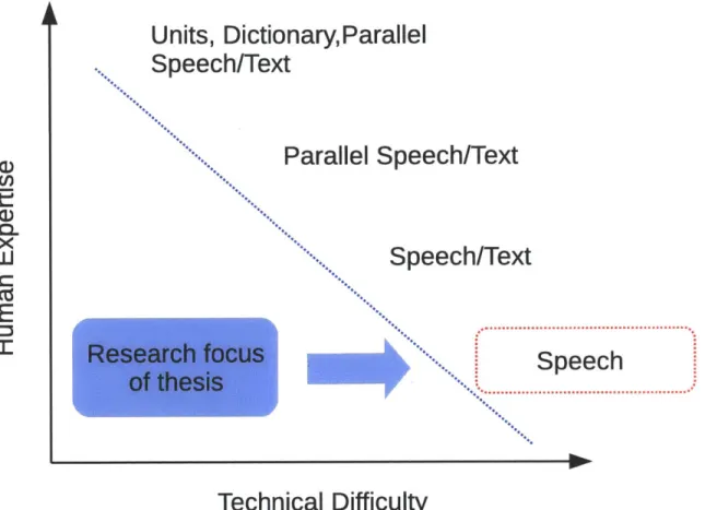
Figure 1-1: Different ASR learning scenarios. By increasing the human expertise (supervision), the technical difficulty becomes smaller for most modern statistical learning frameworks. However, less human expertise generally would cause an increase in the learning difficulty which needs to be carefully addressed and explored. The figure is adapted from [39]. This thesis primarily addresses the speech-only scenario.

summary will be also presented.

1.1 Vision

Although the conventional ASR framework has achieved tremendous success in different applications, there are alternative ways of processing speech data in different learning scenarios [39]. Shown in Figure 1-1, there are four different ASR learning scenarios classified by the different degrees of human supervision. By increasing the human expertise (supervision), the technical difficulty becomes smaller for most modern statistical learning frameworks. However, less human expertise generally

(20)

would cause an increase in the learning difficulty which needs to be carefully addressed and explored. In the following paragraphs, we will describe all four scenarios and point out what scenario this thesis is going to focus on.

The first scenario consists of problems where detailed linguistic resources including parallel speech/text transcription and phoneme-based dictionary are available. Most modern speech systems fall into this scenario and decent speech recognizers can be trained by using the well-known sub-word hidden Markov models (HMMs) [76, 6].

In the second scenario, dictionaries and linguistic units are not provided except for the parallel speech/text transcription. The learning problem becomes harder because the phoneme inventory needs to be automatically learned and the corresponding dictionary needs to be automatically generated. There has been some research aiming to learn acoustically meaningful linguistic units from the parallel speech/test data, such as the Grapheme-based letter-to-sound (L2S) learning [65], Grapheme based speech recognition [30, 69] and the pronunciation mixture models (PMMs) [5].

If only independent speech and text data are available, it is difficult to determine what words exist where in the speech data. In this scenario, it is impossible to build connections between the speech signals and the corresponding linguistic units. However, a few speech processing tasks have been explored and shown to be feasible such as discovering self-organizing units (SOUs) [119], sub-word units [134, 58], etc.

In the scenario where only speech signals are available, speech processing becomes an extreme learning case for machines, often referred to as the zero resource learn-ing scenario for speech

[37].

In recent years, this scenario has begun to draw more attention in the speech research community. Prior research showed that a variety of speech tasks can be done by looking at the speech signal alone, such as discover-ing word-like patterns [98, 120], query-by-example spoken term detection [38], topic segmentation [78, 79, 31] and phoneme unit learning [73], etc.

The latter, speech only scenario is particularly interesting to us for the following reasons:

1. Along with the fast growth of Internet applications and hand-held smart

(21)

Hello, world

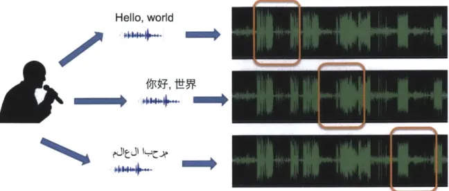
Figure 1-2: Query-by-Example Spoken Term Detection (QE-STD). A user/tester makes spoken queries and the QE-STD system locates occurrences of the spoken queries in test recordings.

hundreds of hours of news broadcasts in many languages have been recorded and stored almost every media provider. Most companies record customer ser-vice calls for future training use. Voice-based applications such as Google Voice Search [43] and Youtube [144] receive a large amount of speech data in every second. However, since none of those speech data has any form of transcrip-tion, it becomes difficult to leverage these data into the conventional highly supervised ASR training paradigm.

2. Transcribing speech data is a long and expensive process [54]. According to a variety of research reports, it is common to take four hours to produce the orthographic transcription of only one hour of speech data without time align-ment [92]. In some acoustic modeling scenarios, in order to produce a time aligned phonetic transcription, it would take a professional linguistic expert a hundred hours to transcribe one hour of speech data [92]. Total cost is esti-mated based on $200 per hour for word level transcription and $2000 per hour for phonetic level transcription.

Therefore, in this thesis, we focus on techniques where only speech data are avail-able, and perform an unsupervised query-by-example spoken term detection

(22)

(QE-STD) task as a means of evaluation. Spoken term detection ((QE-STD) has been an

interesting research topic over many years. Figure 1-2 illustrates the concept of the

QE-STD

task, where a user/tester makes spoken queries and the QE-STD system lo-cates occurrences of the spoken queries in test recordings. Conventional STD systems have developed into two directions. One direction is based on post-processing ASR output, focusing on detecting spoken terms at the recognition text level. The other direction is based on directly modeling speech and spoken terms, detecting spoken terms on the speech segment level without running ASR on every word. Although several systems [109, 140, 124, 62, 21] have demonstrated the effectiveness of both methods, both require a large amount of supervised training. For instance, the post-processing based approach requires an ASR engine trained using supervised speech data, while the model based approach needs enough examples of each spoken term, which can be comparable to the data requirements for a standard speech recognizer. In this thesis, we focus on investigating techniques to perform spoken term detec-tion directly on the speech signal level without using any supervision. Two robust speech feature representations and the corresponding fast matching algorithms will be proposed. We demonstrate that the proposed feature representations can reduce the speaker dependency problem, while maintaining a good level of similarity among spoken term appearances. The fast matching algorithms outperform conventional matching algorithm by a factor of four orders of magnitude.

1.2 Main Contributions

The main contributions of this thesis can be summarized as follows:

Representation. Two different robust feature representations are proposed for

the QE-STD task. One is a Gaussian posteriorgram based features which are speaker independent and can be generated in completely unsupervised conditions. The other is a Deep Belief Network (DBN) posteriorgram based features which can be used to refine the Gaussian posteriorgram features in the unsupervised setting or directly generate posteriorgram features in semi-supervised or supervised settings. The

(23)

fea-sibility and effectiveness of both posteriorgram features are demonstrated through a set of spoken term detection experiments on different datasets.

Matching. Three lower-bounding based fast matching algorithms are proposed

for locating spoken terms on posteriorgram features. Two algorithms can be used in single-threaded computing environments, while the third algorithm is designed to run in multi-threaded computing environments. All three algorithms greatly outperform the conventional Segmental Dynamic Time Warping (S-DTW) algorithm for the

QE-STD task.

1.3 Chapter Summary

The remainder of this thesis is organized as follows:

Chapter 2 provides background knowledge and some pre-existing techniques used in this thesis.

Chapter 3 gives an overview of the proposed Gaussian posteriorgram based

QE-STD framework. Using Gaussian posteriorgram features, a new unsupervised spoken

term discovery system is presented to show that Gaussian posteriorgrams are able to efficiently address the speaker dependency issue in tasks other than QE-STD.

Chapter 4 introduces the new Deep Belief Network (DBN) posteriorgram based

QE-STD framework. Given different levels of speech annotation, three DBN

posteri-orgram configurations are described. The evaluation results on TIMIT and the Babel corpus are reported and discussed. Furthermore, denoising DBN posteriorgrams are presented to show some promising results for QE-STD on noisy speech data.

Chapter 5 presents two fast matching algorithms on posteriorgram features. Both algorithms utilize a lower-bounding idea but operate on different approximation levels. Experiments and comparisons are reported and discussed.

Chapter 6 further explores a fast matching algorithm in a multi-threaded com-puting environment - Graphical Processing Unit (GPU) comcom-puting. A fully parallel lower-bounding based matching algorithm is described. Experimental results on a huge artificially created speech corpus are presented and discussed. In addition,

(24)

effi-cient GPU based DBN training algorithms are described and speed comparisons are presented.

Chapter 7 concludes this thesis and provides discussion of some potential improve-ment of the proposed QE-STD framework.

(25)

Chapter 2 Background

This chapter provides background about the techniques used in the following chapters. The conventional speech feature representation - Mel-scale cepstral coef-ficients (MFCCs) and the most commonly used acoustic model Gaussian Mixture Model (GMM) will be described. The Segmental Dynamic Time Warping (S-DTW) algorithm will be reviewed since it will be used in experiments as a matching method on the speech representations. Finally, we present several speech corpora that are used in the experiments performed in this thesis.

2.1 MFCC Representation

When speech is recorded by a microphone, the signal is first digitized and rep-resented by discrete amplitudes as a function of time given a fixed sampling rate. Most modern speech recording devices have a default sampling rate of at least 16kHz for human speech, while the standard telephone speech coding method only supports 8kHz in order to save transmission bandwidth.

From the statistical learning point of view, with a high sampling rate of 16kHz or 8kHz, it is difficult to process speech directly from the waveform. Therefore, there has been a number of signal processing methods focusing on converting the speech waveform to a short-time spectral representation. A spectral representation has inherent advantages such as having lower dimensionality, yet preserving relevant

(26)

Waveform

0 .2

---E

0 -0.2 L ---0 1 2 3 4

Time

Spectrogram

N5000 0 0.5 1 1.5 2 2.5 3 3.5 4

Time

Figure 2-1: Waveform representation and the corresponding spectrogram representa-tion of a speech segment.

phonetic information

[54].

Mel-frequency cepstral coefficients (MFCCs) are one of the widely used spectral representations for ASR and have become a standard front-end module for feature extraction in most modern ASR systems.

In order to compute MFCCs for a recorded speech signal x[t], the following stan-dard steps are applied.

1. Waveform normalization and pre-emphasis filtering. A common pre-processing

approach is to apply mean and magnitude normalization, followed by a pre-emphasis filter:

Xn[t] = x[t] - mean(x[t]) (2.1)

max Ix[t]|

x,[t| = xn[t] - 0.97xn[t - 1] (2.2)

(27)

trans-form (STFT) is pertrans-formed on the wavetrans-form with a window size of 25ms, and an analysis shift of 10ms. The most commonly used window is the Hamming window

[93].

After the STFT, the speech can be represented in the spectro-gram form, shown in Figure 2-1. In the following chapters, each analysis is often referred as a speech frame.

00

XSTFT[t, k] = x,[t]w[t - mle-i2 rmk/N (2.3)

m=-oo

where w is the Hamming window, N is the number of points for the discrete Fourier transform (DFT) and XSTFT[t, k] is the k-th spectral component at time t.

3. Calculation of Mel-frequency spectral coefficients (MFSCs). The Mel-frequency

filter is designed based on an approximation of the frequency response of inner ear [85]. The Mel-filter frequency response is shown in Figure 2-2. On each speech frame after the STFT, a Mel-frequency filter is used to reduce the spec-tral resolution, and convert all frequency components to be placed according to the Mel-scale.

0--o Mi (k)|IXST FT [t, k]|12

XMFSC[t,i] = 0 0 Mil |' (2.4)

where i denotes the i-th Mel-frequency filter and

|Mil

represents the energy normalizer of the i-th filter.

4. Calculation of discrete cosine transform (DCT). The DCT is then applied to the logarithm of the MFCSs to further reduce the dimensionality of the spec-tral vector. Typically only the first 12 DCT coefficients are kept. Prior research has shown that adding more DCT components does not help increase the qual-ity of the MFCCs for ASR, although more MFCCs are often used for speaker identification tasks [107, 106, 67].

=_0 10loi

(XMFSCti])

_c

(

_ki

(28)

0.8- - 0.6- 0.4- 0.2-01 0 500 1000 1500 2000 2500 3000 3500 4000 Frequency (Hz)

Figure 2-2: Triangular filters placed according to Mel frequency scale. A

Mel-frequency filter is used to reduce spectral resolution, and convert all Mel-frequency com-ponents to be placed according to the Mel-scale.

where M represents the number of Mel-frequency filters and XMFCC[t,

i]

de-notes the i-th MFCC component at time t.

After the above four steps, the calculation of MFCCs given a speech signal is complete. In practice, when using MFCCs in the acoustic modeling, long-term MFCCs features are often considered, such as delta (A) MFCCs and delta-delta

(AA) MFCCs [54]. The A MFCCs are the first derivatives of the original MFCCs

and the AA MFCCs are the second derivatives of the original MFCCs. A common configuration of the modern ASR feature extraction module is to use the original MFCCs stacked with the A and AA features. The original MFCCs are represented

by the first 12 components of the DCT output plus the total energy (+A Energy

(29)

2 I I 1.8 1.6 1.4 1.2 >%1 0.8 k .. . 0.61F 0.4 0.2 F-0' -5 -4 -3 -2 -1 0 1 2 3 4 5 x

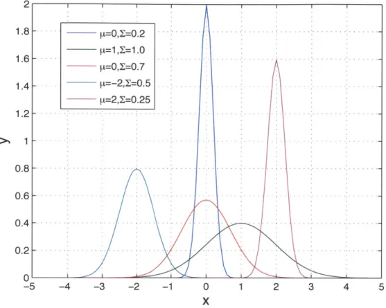
Figure 2-3: A GMM with five Gaussian components with equal weights.

+AA

Energy), which results in a 13+13+13=39 dimensional feature vector for each speech frame.

2.2 Gaussian Mixture Models

The Gaussian Mixture Model (GMM) is a widely used technique for modeling speech features such as MFCCs [101]. A standard GMM with K Gaussian components can be written as

K

P(x) = _{wiN(x; pi, Ej),}

K

wz = 1 (2.6)

where x is the speech observation (e.g., the 39-dimensional MFCCs), wi represents the scaling factor and sums to one, N is a multivariate Gaussian distribution with

[=1,1=1.0 2 -- -... ... . . . . . . . . . . . . . . . . . . ... . . .

(30)

mean y and variance E. Figure 2-3 shows a GMM with five components with equal weights. Considering one Gaussian distribution, given the observation vector x, the log-probability can be written as

log(27r)D _ log(|E|)

(x

- p)TE-1(x - p)

(2.7)

log(N(x;y, E)) = 22.7)

2 2 2

where D is the dimensionality of the observation vector and

|El

denotes the

deter-minant of the covariance matrix. Given a speech corpus X = X1, z2,.-. , XN, the log-probability of the entire speech corpus is

N

log(N(xi; y, E)) (2.8)

2.3 Dynamic Time Warping

Dynamic Time Warping (DTW) is a well-known dynamic programming technique for finding the best alignment between two time series patterns [54]. DTW became popular in the speech research community from the late 1970's to mid 1980's, and was used for both isolated and connected-word recognition with spectrally-based represen-tations such as Linear Prediction Coding (LPC) [101]. DTW allowed for minor local time variations between two speech patterns which made it a simple and efficient search mechanism. Over time, DTW-based techniques were supplanted by hidden Markov models (HMMs) which were a superior mathematical framework for incor-porating statistical modeling techniques. However, DTW-based search has remained attractive and has been used by researchers incorporating neural network outputs for ASR [74, 48], and more recently for scenarios where there is little, if any, training data to model new words [27, 139, 98].

One attractive property of DTW is that it makes no assumptions about underly-ing lunderly-inguistic units. Thus, it is amenable to situations where there is essentially no annotated data to train a conventional ASR engine. In this thesis, we are interested in developing speech processing methods that can operate in such unsupervised con-ditions. For the QE-STD task, we have an example speech query pattern and we wish

(31)

to find the top K nearest-neighbor (KNN) matches in some corpus of speech utter-ances. DTW is a natural search mechanism for this application, though depending on the size of the corpus, there can be a significant amount of computation involved in the alignment process.

Formally, given two time series P and

Q

with length n and m

P = plip2, -- ,Pn (2.9)

Q

= qi, q2, - m (2.10)

The DTW can be used to construct an optimal alignment A between P and

Q

as

A= #1,# , OK (2.11)

where K is the warping length and each

#i

is a warping pair

#i

= (#0,

#b)

which aligns pa with qb according to the pre-defined distance metric D(pa, q). Note that

both Pa and qb can be multi-dimensional as long as the distance function D can be properly defined. It is clear that the warping begins with

#1

= (pi, q1) and ends with

#K(pn,

qm) and the length K is bounded by max(n, m) < K < n+ m. The DTW can

find the optimal warping path A given the following objective function

KA

DTW(P, Q)

=

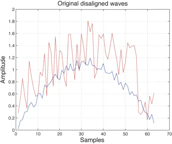
A= min ZD(4(A)) (2.12)

where <D denotes the set of all possible warping paths and 4(A)i represents the i-th warping pair of i-the warping pai-th A. Figure 2-4 shows two sinusoid signals wii-th random Gaussian noise. If we perform DTW on those two signals and find an optimal alignment in terms of Euclidean distance, the alignment is shown in red in the middle sub-figure of Figure 2-5. Lighter pixels denote smaller Euclidean distance, while darker pixels denote larger distance.

One important property of the DTW alignment is that the warping process must be monotonically increasing and every pi and qj must appear in the optimal alignment

(32)

Original disaligned waves

2 1 .8 -.-.-.-1 .6 -.-.-.-.-1.4 -0) 1.2

E

<0.8 0.6 --0.4 - - - -0 .2 -.- . -.-.-.-.-.-0 0 10 20 30 40 50 60 70

Samples

Figure 2-4: Two sinusoid signals with random Gaussian noise. DTW is used to find an optimal alignment between those two signals in terms of Euclidean distance.

A

at least once. This property leads to an efficient dynamic programming algorithm that computes the optimal warping path

A

in 0(nm). Specifically, the algorithm starts from solving a minimum subsequence of P and

Q

and grows the minimum subsequence iteration by iteration until the full optimal warping path is found. For the above time series P and

Q,

the core idea of computing DTW can be illustrated

by a cost matrix C of size n by m. Each element Cjj represents the minimum total

warping path cost/distance from (pi, q1) to (pi, qj) and it can be calculated as

Ci_1,j

C,3 = D(pi, qj) + min C ' _1 (2.13)

Ci is

(33)

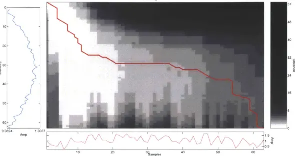
DTW Alignment 30-24 40 16 50-- 8 000 0.0894 1 3037 -AmpII I 183 0.5 10 20 3Lamples 40 0 60

Figure 2-5: The optimal alignment of the two sinusoid signals after performing DTW with Euclidean distance as the local distance metric. The red line represents the optimal alignment. Lighter pixels denote smaller Euclidean distance, while the darker pixels denote lager Euclidean distance.

C1,1, C can be constructed row by row and the total cost/distance of the optimal warping path is Cm.

2.3.1 Segmental Dynamic Time Warping

Segmental Dynamic Time Warping (S-DTW) is a segmental variant of the origi-nal DTW algorithm that finds optimal alignments among subsequences of two time series

[98].

The S-DTW is a two-staged algorithm. In the first stage, the S-DTW finds local alignments among subsequences of the input two time series. In the second stage, a path refinement approach is used to eliminate lower distortion regions in the local alignments found in the first stage.

S-DTW defines two constraints on the DTW search. The first one is the commonly used adjustment window condition [112]. In our case, formally, suppose we use the same above two time series A and B, the warping pair w(.) defined on a n x m timing difference matrix is given as wi = (i,

jA)

where ik and

jA

denote the k-th coordinate of the warping path. Due to the assumption that the duration fluctuation is usually

(34)

small in speech [112], the adjustment window condition requires that

lik

- jkl < R.

This constraint prevents the warping process from going too far ahead or behind in either A or B.

The second constraint is the step length of the start coordinates of the DTW search. It is clear that if we fix the start coordinate of a warping path, the adjustment window condition restricts not only the shape but also the ending coordinate of the warping path. For example, if i1 = 1 and Ji = 1, the ending coordinate will be

iend = n and jend E (1 + n - R, 1 + n + R). As a result, by applying different start

coordinates of the warping process, the difference matrix can be naturally divided into several continuous diagonal regions with width 2R

+

1, shown in the Figure 2-6. In order to avoid the redundant computation of the warping function as well as

taking into account warping paths across segmentation boundaries, an overlapped sliding window strategy is usually used for the start coordinates (sl and s2 in the figure). Specifically, with the adjustment window size R, every time we move R steps forward for a new DTW search. Since the width of each segmentation is 2R

+

1, the

overlapping rate is 50%.

By moving the start coordinate along the i and

j

axis, a total of [ I +

L-R

1

]

warping paths can be obtained, each of which represents a warping between two subsequences in the input time series.

The warping path refinement is done in two steps. In the first step, a length L constrained minimum average subsequence finding algorithm [77] is used to extract consecutive warping fragments with low distortion scores. In the second step, the extracted fragments are extended by including neighboring frames below a certain distortion threshold a. Specifically, neighboring frames are included if their distortion scores are within 1 + a percent of the average distortion of the original fragment.

In this thesis, for the QE-STD task, we use a modified single-sided S-DTW algo-rithm which finds optimal alignments of a full time series against all subsequences in another time series. For the spoken term discovery task, the full S-DTW algorithm is used.

(35)

s2

V.V

s3

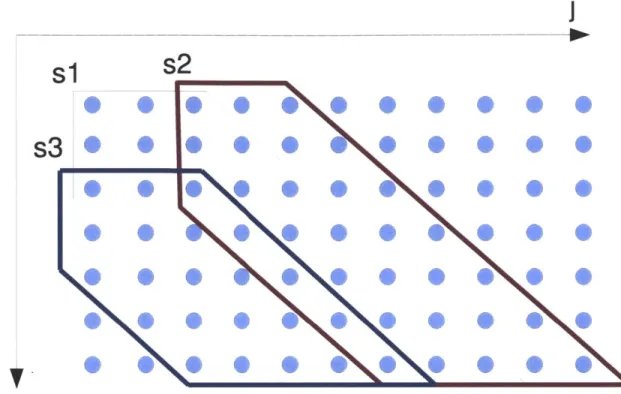
Figure 2-6: An illustration of S-DTW between two utterances with R = 2. The

blue and red regions outline possible DTW warping spaces for two different starting times. In order to avoid the redundant computation of the warping function as well as taking into account warping paths across segmentation boundaries, an overlapped sliding window strategy is usually used for the start coordinates (s1 and s2 in the figure).

2.4 Speech Corpora

Four speech corpora are used in the experiments in this thesis. A brief overview of each speech corpus will be described in the following sections.

2.4.1 TIMIT

The TIMIT corpus consists of read speech recorded in quiet environments. It is designed for acoustic-phonetic studies and for the development and evaluation of ASR systems. The TIMIT corpus contains broadband recordings of 630 speakers of 8 major dialects of American English. Each speaker reads 10 phonetically rich sentences, include 2 "sa" sentences representing dialectal differences, 5 "sx" sentences covering phoneme pairs and 3 "si" sentences that are phonetically diverse. The TIMIT

(36)

transcriptions have been hand verified, including time-aligned orthographic, phonetic and word transcriptions. The TIMIT corpus is well-known for its balanced phoneme inventory and dialectal coverage [71].

The TIMIT corpus is divided into three sets. The training set contains 3,696 utterances from 462 speakers. The development set consists of 400 utterances from

50 speakers. The test set includes 944 utterances from 118 speakers. A commonly

used core test set for ASR evaluations is a subset of the full test set, containing 192 utterances from 24 speakers. The results in this thesis are reported on the full test

set.

2.4.2 NTIMIT

NTIMIT is a noisy version of the TIMIT corpus. It was collected by transmitting all 6,300 original TIMIT recordings through a telephone handset and over various channels in the NYNEX telephone network and re-digitizing them [57]. The record-ings were transmitted through ten Local Access and Transport Areas, half of which re-quired the use of long-distance carriers. The re-recorded waveforms were time-aligned with the original TIMIT waveforms so that the TIMIT time-aligned transcriptions can be used with the NTIMIT corpus as well. The training/development/test set division is the same as the original TIMIT corpus. This corpus is used for evaluating spoken term detection in noisy conditions in this thesis.

2.4.3 MIT Lecture

The MIT Lecture corpus consists of more than 300 hours of speech data recorded from eight different subjects and over 80 general seminars [41]. In most cases, the data is recorded in a classroom environment using a lapel microphone. The recordings were manually transcribed including tags for disfluencies. The vocabulary size is 27,431 words. A standard training set contains 57,351 utterances and a test set is comprised of 7,375 utterances.

(37)

evaluations for three reasons. First, the data is comprised of spontaneous speech as well as many disfluencies such as filled pauses, laughter, false starts and partial words. Second, since the data was recorded in a classroom environment, there are many non-speech artifacts that occur such as background noise and students' random talking. Third, some lecture specific words are uncommon and can result in significant out-of-vocabulary problems. This corpus is used in both spoken term detection and spoken term discovery experiments in this thesis.

2.4.4 Babel Cantonese

The Babel Cantonese corpus contains a training set of 50 hours of telephone speech and a test set of 200 minutes of telephone speech. The speech data was produced by presenting a topic to native Cantonese speakers and asking them to make a 10-minute long telephone call about the topic. The telephone calls were recorded by different telephone carriers, which results in very different channel noise levels for each call. This corpus is used to demonstrate the language independent feature of the proposed spoken term detection system in this thesis.

2.5 Summary

In this chapter, we described some well-established speech processing techniques that will be utilized in this thesis. We first discussed how to calculate the MFCC features for speech. Next, we presented a common acoustic modeling framework using GMMs on MFCC features. The well-known DTW and its variant S-DTW algorithms were reviewed. In the end, we described four datasets that will be used in the following

(38)

(39)

Chapter 3 Unsupervised Gaussian

Posteriorgram

In this chapter, we present an overview of the unsupervised Gaussian posterior-gram framework. The Gaussian posteriorposterior-gram framework was our first attempt to represent speech in the posteriorgram form without using any supervised annota-tion. The core idea is to train a Gaussian mixture model (GMM) without using any supervised annotation, and represent each speech frame by calculating a posterior distribution over all Gaussian components. A modified DTW matching algorithm can be used to evaluate the similarity between two speech segments represented by Gaussian posteriorgrams in terms of an inner-product distance. The entire process is completely unsupervised and does not depend on speakers. After the success of using Gaussian posteriorgrams on a spoken term discovery task [147], a query-by-example spoken term detection task was then performed [146], which further demonstrate the effectiveness of using the Gaussian posteriorgram as a robust unsupervised feature representation of speech.

3.1 Posteriorgram Representation

The posteriorgram representation for speech data was inspired by the widely used posterior features in template-based speech recognition systems [48, 32, 3, 4]. For

(40)

example, in the Tandem [48, 32] speech recognition system, a neural network is dis-criminatively trained to estimate posterior probability distributions across a phone set. The posterior probability for each frame on each phone class is then used as the feature input for a conventional Gaussian mixture model with hidden Markov model (GMM-HMM) based speech recognition system. The motivation behind using poste-rior features instead of spectral features is that by passing through a discriminatively trained classifier, speaker dependent, unevenly correlated and distributed spectral fea-tures are converted into a simpler; and speaker-independent statistical form while still retaining phonetic information. The subsequent modeling process can focus more on capturing the phonetic differences rather than directly dealing with the speech spec-trum. Previous results showed that a large improvement in terms of word recognition error rate could be obtained [48, 32].

The most recent work by Hazen et al. [46] showed a spoken term detection sys-tem using phonetic posteriorgram sys-templates. A phonetic posteriorgram is defined by a probability vector representing the posterior probabilities of a set of pre-defined phonetic classes for a speech frame. By using an independently trained phonetic rec-ognizer, each input speech frame can be converted to its corresponding posteriorgram representation. Given a spoken sample of a term, the frames belonging to the term are converted to a series of phonetic posteriorgrams by phonetic recognition. Then, Dynamic Time Warping (DTW) is used to calculate the distortion scores between the spoken term posteriorgrams and the posteriorgrams of the test utterances. The detection result is given by ranking the distortion scores.

To generate a phonetic posteriorgram, a phonetic classifier for a specific language is needed. In the unsupervised setting, there is no annotated phonetic information that can be used to train a phonetic classifier. Therefore, instead of using a supervised classifier, our approach is to directly model the speech using a GMM without any supervision. In this case, each Gaussian component approximates a phone-like class.

By calculating a posterior probability for each frame on each Gaussian component,

we can obtain a posterior feature representation called a Gaussian posteriorgram. While the discriminations of a Gaussian posteriorgram do not directly compare

(41)

to phonetic classes, the temporal variation in the posteriorgram captures the impor-tant phonetic information in the speech signal, providing some generalization to a purely acoustic segmentation. With a Gaussian posteriorgram representation, some speech tasks could be performed without any annotation information. For example, in a query-by-example spoken term detection system, the input query which is rep-resented by a series of Gaussian posteriorgrams can then be searched in the working data set which is also in the Gaussian posteriorgram representation [146]. In a spoken term discovery system, given a speech recording, if we want to extract frequently used words/short phrases, a Gaussian posteriorgram can be used to represent the entire recording, and a pattern matching algorithm can be applied to find similar segments of posteriorgrams [147]. In this chapter, we will demonstrate how the Gaussian pos-teriorgram can be used as a robust, speaker independent representation of unlabeled speech data.

3.2 Gaussian Posteriorgram Generation

If a speech utterance S contains n frames S = (f, f,--- ,

f,),

then the

Gaus-sian posteriorgram for this utterance is defined by GP(S) = (1, q2, - , n). The

dimensionality of each j is determined by the number of Gaussian components in the GMM, and each q can be obtained by

q = {P(Cilfi), P(C 2|f),... , P(CMQf)} (3.1)

where the j-th dimension in q represents the posterior probability of the speech frame f, on the j-th Gaussian component Cj. m is the total number of Gaussian components.

The GMM is trained on all speech frames without any transcription. In this work, each raw speech frame is represented by the first 13 Mel-frequency cepstrum coeffi-cients (MFCCs). After pre-selecting the number of desired Gaussian components, the K-means algorithm is used to determine an initial set of mean vectors. Then,

(42)

Spectrogram 6000 0.5 1 15 2 215 3 3.5 4 Time Gaussian posteriorgram 0 40 50 0.5 1 1.5 2 2.5 3 3.5 4 Ti me

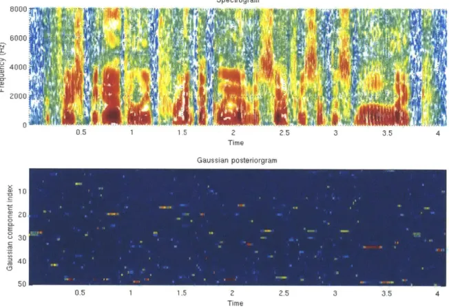
Figure 3-1: A spectrogram (top) and Gaussian posteriorgram

(bottom)

of a TIMIT utterance. To generate posteriorgrams, a 50-component GMM was trained on 13-MFCC features on the standard TIMIT training set. In the bottom figure, the y axis denotes the Gaussian component indices. Each pixel

(x, y) represents the posterior

probability of Gaussian component y for speech frame x. Blue pixels denote lower probabilities while red pixels indicate higher probabilities. It can be seen from the bottom figure that Gaussian posteriorgrams are able to represent phonetically similar speech frames. For example, the frames from 3.25s to 3.48s have the most posterior probability mass on the 3 3Td GMM component, while the frames from 1.30s to 1.37s have the most posterior probability mass on 1 7th GMM component and some mass on the 4 3rd component.

(43)

Figure 3-1 shows an example of the Gaussian posteriorgram representation for a TIMIT utterance. The top figure is the spectrogram representation. In the bottom figure, the y axis denotes the Gaussian component indices. Each pixel (x, y) repre-sents the posterior probability of Gaussian component y for speech frame x. Blue pixels denote lower probabilities while red pixels indicate higher probabilities. It can be seen from the bottom figure that Gaussian posteriorgrams are able to represent phonetically similar speech frames. For example, the frames from 3.25s to 3.48s have the most posterior probability mass on the 3 3rd GMM component, while the frames

from 1.30s to 1.37s have the most posterior probability mass on 1 7 th GMM

compo-nent and some mass on the 4 3 rd component. By looking at the spectrogram, we could

derive that the 3 3rd GMM component probably corresponds to back vowels, while the

1 7th and 4 3rd GMM components probably correspond to fricatives.

3.3 Analysis of Gaussian Posteriorgram

In Gaussian posteriorgram generation, we assume that through unsupervised GMM training, each Gaussian component can be viewed as a self-organizing pho-netic class. To validate this assumption, a phopho-netic histogram analysis is applied to visualize the underlying acoustically meaningful information represented by each Gaussian component. Specifically, after unsupervised GMM training, each speech frame is artificially labeled by the index of the most probable Gaussian component. Since the TIMIT dataset provides a time-aligned phonetic transcription, for each Gaussian component, we can calculate the normalized percentage of how many times one Gaussian component represents a particular phone. By drawing a bar for every TIMIT phone for one Gaussian component, we can have a histogram of the underlying phonetic distribution of that Gaussian component.

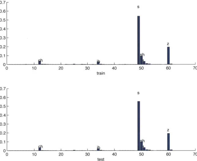
Figure 3-2 shows the phonetic distribution of frames assigned to Gaussian com-ponent 13. Each bar in the figure represents the percentage of time that this cluster represents a phone class in TIMIT. Note that the size of the TIMIT phone inventory is 61. The top figure is the histogram of the training set, while the bottom

(44)

sub-0.7 0.6- 0.5- 0.4- 0.3- 0.2-0.1 -0 -0 0.7- 0.6- 0.5- 0.4- 0.3- 0.2-0.1 -0 -S z 10 20 30 40 50 60 70 train s z 0 10 20 30 40 50 60 70 test

Figure 3-2: This figure illustrates the phonetic distribution of frames assigned to Gaussian component 13. Each bar in the figure represents the percentage of times that this cluster represents a phone. The top sub-figure is on the training set, while the bottom sub-figure is on the test set. It is clear that this cluster mainly represents fricatives and affricates.

figure is the histogram of the test set. It is clear that this cluster mainly represents fricatives and the release of affricates.

Figure 3-3 illustrates the phonetic distribution of frames assigned to Gaussian component 41. Since most bars are labeled as vowels or semi-vowels, this cluster mainly represents vowels and semi-vowels. Note that most vowels are front-vowels.

Figure 3-4 illustrates the phonetic distribution of frames assigned to Gaussian component 14. This cluster mainly represents retroflexed sound such as /r/, /er/ and

/axr/.

(45)

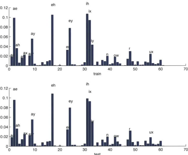
eh ih 0.12 - ae i 0.1 -ey 0.08-0.06- ay iy 0 0 4 - a h a xe _r1U 0.02 nx]U 0 0 10 20 30 40 50 60 70 train eh ih 0.12 - ae i 0.1 -ey 0.08-0.06- ay 0.04 ah e r 0.02 W U 0 10 20 30 40 50 60 70 test

Figure 3-3: This figure illustrates the phonetic distribution of frames assigned to Gaussian component 41. Each bar in the figure represents the percentage of times that this cluster represent a phone. The top sub-figure is on the training set, while the bottom sub-figure is on the test set. Since most bars are labeled as vowels or semi-vowels, it is clear that this cluster mainly represents vowels and semi-vowels.

(46)

er axr

I

- - --- -- ---- -10 20 30 train 40 er axr MI -91 . 10 20 30 test 40

Figure 3-4: This figure illustrates the phonetic distribution of frames assigned to Gaussian component 14. Each bar in the figure represents the percentage of times that this cluster represent a phone. The top sub-figure is on the training set, while the bottom sub-figure is on the test set. This cluster mainly represents retrofled sound. 0.35 0.3 -0.25 0.2 r 0.15 0.1-0.05 0 0 0.3 0.25 50 60 0.2 1 70 0. 15 -0.1

i

0.05 _a~o U-..-. U' 0 50 60 70

---

--

I

$ 0.35 r

Unsupervised speech processing with applications to query-by-example spoken term detection

Unsupervised Speech Processing with Applications

to Query-by-Example Spoken Term Detection

by

Yaodong Zhang

Submitted to the Department of Electrical Engineering and Computer

Science

FARCH1ES

in partial fulfillment of the requirements for the degree o

Doctor of Philosophy

at the

MASSACHUSETTS INSTITUTE OF TECHNOLOGY

February 2013

©

Massachusetts Institute of Technology 2013. All rights reserved.

Author ...

...

...

Department of Electrical Engineering and Computer Science

Jan 10, 2013

C ertified by ...

1****

James R. Glass

Senoir Research Scientist

Thesis Supervisor

A ccepted by ...

Chairman, Department Committee on Graduate Theses

Unsupervised Speech Processing with Applications to

Query-by-Example Spoken Term Detection

by

Yaodong Zhang

Abstract

Acknowledgments

Contents

List of Figures

#

List of Tables

#

Chapter 1

Introduction

Units, Dictionary,Parallel

Speech/Text

-

Parallel Speech/Text

Speech/Text

w

E

Speech

Technical Difficulty

1.1

Vision

[37].

QE-STD

1.2

Main Contributions

1.3

Chapter Summary

Chapter 2

Background

2.1

MFCC Representation

Waveform

---E

Time

Spectrogram

Time

[54].

[93].

|Mil

(XMFSCti])

(

i]

+AA

2.2

Gaussian Mixture Models

(x

(2.7)

|El

2.3

Dynamic Time Warping

_FARCH1ES

_{James R. Glass}