2019
Acceptée sur proposition du jury
pour l’obtention du grade de Docteur ès Sciences par
Anna ARCHETTI
Présentée le 25 juin 2019
Thèse N° 9630
fluorescence microscopy of sub-cellular structures
Prof. C. S. Brès, présidente du jury Prof. S. Manley, directrice de thèse Prof. A. Diaspro, rapporteur Prof. T. Huser, rapporteur Prof. C. Galland, rapporteur à la Faculté des sciences de base
Laboratoire de biophysique expérimentale Programme doctoral en photonique
Abstract
Super-resolution fluorescence microscopy is widespread, owing to its demonstrated ability to resolve dynamical processes within cells and to identify the structure and position of specific proteins in the interior of protein complexes. Nowadays, subcellular features can be routinely resolved at the nanoscopic scale thanks to the accessibility of straightforward sample-preparation protocols, simple hardware tools, and open source software. Building on its ability to investigate large-scale macromolecules networks in their natural environment with high resolution, fluorescence microscopy is further evolving by the development of quantitative and high-throughput methods to characterize such networks. Previous implementations of high-throughput microscopy made use of imaging sequentially smaller fields of view (FOV), which makes axial alignment a challenge and extends the imaging time. In our work, we circumvent these problems with our large FOV systems, which are based on flat-field sample illumination over large areas, combined with a CMOS-camera.
In this thesis, I present a waveguide platform designed to image a wide area with low background by mean of total internal reflection fluorescence (TIRF) excitation. The waveguide chips for this platform were fabricated at the center of micro-nano technology (CMi) at EPFL, in collaboration with the group of Aleksandra Radenovic (specifically with Evgenii Glushkov). The resulting waveguide-TIRF system is specifically optimized for applications where easy and repetitive buffer exchange is needed.
To achieve large and uniform TIRF excitation, I studied some fundamental parameters of the waveguide, developing specific code to simulate, at the first order, its behavior. I then extended light propagation solutions adopted in the field of integrated photonics to our waveguide chip fabrication process. To easily integrate the chip within the commercial stage of an upright microscope, I designed a novel chip holder that ensures aqueous solution sealing, mitigates the presence of scatter light in the imaging area, and facilitates the waveguide alignment during the input beam-coupling phase.
On the analysis side, the need for computational tools that are specific to fluorescence microscopy is continuously growing, due to the fact that this technique heavily relies on the treatment of large quantities of data. The automated analysis of images is a fundamental step of the measurement process, necessary for unbiased quantification and
4
statistical validation, especially where repetitive visual inspection would be impractically long. This is particularly critical for single molecule localization microscopy (SMLM), where the quality of the reconstructed super-resolved image actually is a trade-off between the algorithm localization precision and its speed, a key element considering the need of processing tens of thousands of large images to generate the final, super-resolved one. In this work, I present a series of computational tools for CMOS camera characterization developed for large flat-field STORM microscopy, a 3D SMLM reconstruction software specific for Double-Helix (DH) point spread function (PSF) and a set of cell shape analysis tools to study C.Crescentus shape dynamics.
KEYWORDS:
super-resolution fluoresce microscopy, TIRF, waveguide micro-nano fabrication, 3D single molecule analysis, bacteria cell shape, image processing
Sommario
La microscopia in fluorescenza a super-risoluzione si è largamente diffusa grazie alla sua dimostrata abilità nel riuscire a risolvere processi dinamici nelle cellule e a discernere la struttura e posizione di specifiche proteine all’interno di complessi proteici.
Tale tecnica si è affermata grazie ad uno sforzo interdisciplinare che ha portato, da un lato, allo sviluppo e validazione di protocolli efficaci per la preparazione dei campioni biologici e, dall’altro, allo sviluppo e diffusione di strumenti ottici innovativi e software open-source. Oggigiorno la microscopia in fluorescenza si sta ulteriormente sviluppando, con l’obbiettivo di permettere uno studio di campioni biologici sempre più estesi con alta risoluzione e alta efficienza.
Lo studio e l’analisi di grandi numeri di sub-campioni viene solitamente eseguito prendendo immagini consecutive di porzioni adiacenti dell’intero campione. Questo approccio, però, richiede un non banale riallineamento assiale per ogni movimento sul piano del capione, ed implica un allungamento del tempo di imaging. I due sistemi che abbiamo sviluppato nel nostro laboratorio permettono invece di analizzare contemporaneamente più sub-campioni, grazie all’estensione dell’illuminazione ad un’area più ampia, senza perdere i requisiti di unifomità e irradianza. La cattura di immagini più estese è stata possibile anche grazie all’utilizzo camere CMOS commercialmente disponibili con un più alto numero di pixels, a parità di frame rate, rispetto alle camere EMCCD precedentemente adottate in questo campo.
In questo lavoro, presento una piattaforma per microscopia in fluorescenza basata su guide-d’onda che permettono di illuminare il campione con un campo evanescente uniforme. La fabbricazione delle guide-d’onda è stata realizzara presso il centro di micro-nano fabbricazione (CMi) dell’EPFL in collaborazione con il gruppo di Aleksandra Radenovic (in particolare con Evgenii Glushkov).
Il campo generato dalla luce rifratta all’interfaccia tra la guida-d’onda e il campione genera una sezionamento (TIRF) ottico del campione che è ragionevolmente uniforme lungo tutta la superficie della guida-d’onda a contatto con il campione. Tale piattaforma è stata ottimizzata per permettere uno scambio veloce di soluzioni acquose. Per ottenere un campo evanescente uniforme e largo ho studiato alcuni parametri fondamentali della guide-d’onda, sviluppando il necessario codice per simularne il comportamento in prima
6
approssimazione. Inoltre ho esteso soluzioni tipicamente adottate nell’ambito della fotonica al processo di fabbricazione delle nostre d’onda. Per integrare le guide-d’onda nel microscopio, ho inoltre progettato un supporto meccanico che potesse non solo allineare facilmente le guide-d’onda con il fascio laser, ma che potesse anche trattenere la soluzione aquosa e schermare la scattering generato nell’area di accoppiamento tra la guida-d’onda ed il laser.
Lo sviluppo di strumenti computazionali specifici per microscopia in fluorescenza é un bisogno in continua crescita, in quanto tale tecnica si basa sul trattamento di grandi quantità di dati, richiedendo una sempre più elevata capacità di analisi.
L’analsisi automatizzata di immagini è infatti fondamentale per una estrapolazione quantitativa e imparziale dei dati, attraverso un campionamento multiplo statisticamente rilevante che richiederebbe tempi irragionevolmente lunghi se effettuato per ispezione visuale diretta. Inoltre, nel campo della microscopia basata sulla localizzazione di singole molecole (SMLM), i software sono fondamentali per poter ricostruire un’immagine super-risolta a partire da decine di migliaia di immagini di milioni di pixels ciascuna, e possono influenzare notevolmente la qualità dell’immagine finale.
In questo lavoro, presento quindi una serie di metodi computazionali sviluppati a partire da una serie di funzioni MATLAB che ho scritto per caratterizzare una CMOS camera accoppiata ad un microscopio STORM basato su un sistema di illuminazione uniforme a vasto campo. Ho inoltre sviluppato una completa pipeline per processare i dati di singole molecole (SM) e ricostruirne un’immagine super-risolta in tre dimensioni. L’informazione assiale sulla posizione della molecola è codificata nella forma della sua point spread function (PSF): infatti la point spread function (PSF) delle molecole è caratterizzata da due lobi che disegnano una doppia elica (double helix - DH) muovendo le molecole nella direzione assiale. Infine, presento una serie di funzioni volte ad analizzare la dinamica della forma cellulare del C.Crescentus.
i
Index
ABSTRACT ... 3 SOMMARIO ... 5 INDEX... I LIST OF TABLES AND FIGURES ... III PART I INTRODUCTION TO SUPERRESOLUTION FLUORESCENCE MICROSCOPY ... 1—1 1SUPER-RESOLUTION PRINCIPLES, METHODS AND LIMITATIONS ... 1—3
1.1 Single Molecule Localization Microscopy (SMLM) ... 1—5
1.1.1 SMLM with photo-switching fluorophores ... 1—5 1.1.2 3D SMLM approaches ... 1—8 1.1.3 DNA Points Accumulation for Imaging in Nanoscale Topography (DNA-PAINT) ... 1—10
1.2 Structured illumination microscopy (SIM) ... 1—13
2IMAGE QUALITY LIMITATIONS IN SMLM ... 2—1
2.1 Illumination aspects critical for image quality ... 2—1
2.1.1 Global field flattening with Köhler integrator or beam shaping elements ... 2—2 2.1.2 Local speckles and interference fringes homogenization ... 2—3
2.2 Optical sectioning techniques ... 2—6
2.2.1 TIRF illumination ... 2—7 2.2.2 Light sheet illumination ... 2—9
2.3 Single molecule localization precision ... 2—14
2.3.1 3D SMLM DH-PSF localization algorithms ... 2—18
PART II APPLICATIONS AND AIMS OF THIS WORK ... 2—23 3RESOLVING BACTERIAL CELL SHAPE DYNAMICS ... 3—25
3.1 Principles of C. crescentus constriction rate modulation in cell shape dynamics ... 3—25
3.1.1 Cell size regulation... 3—28
3.2 Aims of this work: cell shape parameters analysis ... 3—29
3.2.1 Development of an automated image processing method and cell dynamic simulator ... 3—30 3.2.2 Development of 3D Double-Helix PSF software ... 3—32
4HIGH-THROUGHPUT NANOSCOPY OF SUBCELLULAR STRUCTURE: LARGE FLAT FIELD STORM AND PAINT ... 4—35
4.1 Aim of this work: CMOS camera characterization for MLE sCMOS-specific algorithm ... 4—35 4.2 Aim of this work: development of a waveguide-based platform for DNA-PAINT ... 4—39
PART III METHODS DEVELOPMENT AND RESULTS ... 4—41 5RESOLVING BACTERIAL CELL SHAPE DYNAMICS ... 5—43
5.1 Bacteria cell image processing: sDaDa ... 5—44 5.2 Bacteria pole shape dynamics simulator ... 5—46 5.3 3D DH-PSF image reconstruction: StormChaser ... 5—49
6LARGE FLAT FIELD STORM ... 6—57
6.1 CMOS camera noise and characterization ... 6—58 6.2 Maximum Likelihood Localization Estimation (MLE) ... 6—61
7LARGE FLAT FIELD WAVEGUIDE-PAINT ... 7—65
7.1 Waveguide Chip design ... 7—65 7.2 Chip holder and Microscope design ... 7—71 7.3 Waveguide DNA-PAINT imaging of cells and DNA origami ... 7—73
7.3.1 Sample preparation ... 7—73 7.3.2 Imaging and data analysis ... 7—79
ii 8 8—83
8.1 Cell shape image analysis automation ... 8—83 8.2 Flat-field illumination platform: prospective ... 8—84 8.3 Waveguide-TIRF: prospective ... 8—85
APPENDIX ... 8—87 A. WAVEGUIDE PARAMETERS STUDY ... 8—89 B. CHIP HOLDER CAD DESIGN ... 8—90 C. CHIP FABRICATION ... 8—91 BIBLIOGRAPHY ... II CURRICULUM VITAE ... XIV
Personal information ... xiv
Work Experience ... xiv
Education ... xv
Skills ... xv
Interests ... xvi
Publications ... xvi
iii
List of tables and figures
TablesTABLE 1-1 SUPER-RESOLUTION LIGHT MICROSCOPY METHODS. 1—4
TABLE 2-1 LIGHT-SHEET MICROSCOPY METHODS COMPATIBLE WITH SMLM. 2—13
TABLE 5-1 3D DH-PSF SOFTWARE COMPARISON AT THE SMLM CHALLENGE 2016. 5—53
TABLE 6-1 SCMOS ZYLA 4.3 ANDOR CHARACTERIZATION. 6—60
TABLE 7-1 WAVEGUIDE-PAINT EXPERIMENTAL CONDITIONS AND RESULTS. 7—79
TABLE D-1 WAVEGUIDE FABRICATION PROCESS FLOW. 8—91
Figures
FIGURE 1-1 – VISUALIZATION OF THE IMAGING PROCESS. 1—3
FIGURE 1-2 – SINGLE MOLECULE LOCALIZATION MICROSCOPY CONCEPT. 1—6
FIGURE 1-3 – 3D SMLM APPROACHES. 1—8
FIGURE 1-4 – 3D-PSF SIMULATED DATASET 1—9
FIGURE 1-5 – DNA-PAINT SAMPLE SCHEME. 1—10
FIGURE 1-6 – DNA-ORIGAMI CREATION PRINCIPLE. 1—11
FIGURE 1-7 – DNA-PAINT EXPERIMENTAL PARAMETERS AFFECTING THE IMAGING PERFORMANCES. 1—12
FIGURE 1-8 – OPTICAL SECTIONING CAN BE OBTAINED BY LIGHT SHEET OR TIRF APPROACHES. 1—13
FIGURE 1-9 – STRUCTURED-ILLUMINATION CONCEPT. 1—14
FIGURE 1-10 – NONLINEAR FLUORESCENCE EMISSION INTRODUCES HIGH FREQUENCY HARMONICS. 1—14
FIGURE 2-1 – A KOHLER INTEGRATOR. 2—2
FIGURE 2-2 – FLAT-FIELD ILLUMINATION EMPLOYING BEAM SHAPER DIFFRACTIVE ELEMENTS. 2—3
FIGURE 2-3 – SPECKLES AND INTERFERENCE FRINGES HOMOGENIZATION APPROACHES. . 2—4
FIGURE 2-4 – FLAT-FIELD TIRF ILLUMINATION USING AXICON LENS. 2—5
FIGURE 2-5 – OBJECTIVE TIRF LIMITATIONS. 2—6
FIGURE 2-6 – PRISM-TIRF AND OBJECTIVE-TIRF CONFIGURATIONS. 2—7
FIGURE 2-7 – CLASSICAL OBJECTIVE-TIRF AND WAVEGUIDE-TIRF APPROACHES. 2—8
FIGURE 2-8 – LIGHT SHEET APPROACH LIMITS. 2—9
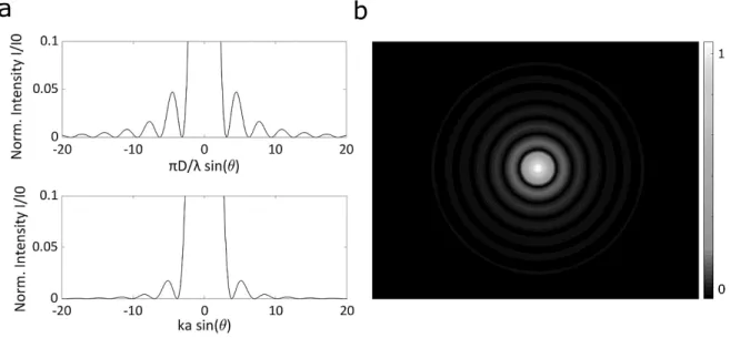
FIGURE 2-9 – BEAM PROPAGATION FROM RECTANGULAR AND CIRCULAR APERTURE. 2—12
FIGURE 2-10 – DEPENDENCE OF THE LOCALIZATION ACCURACY ON THE PIXEL SIZE. 2—17
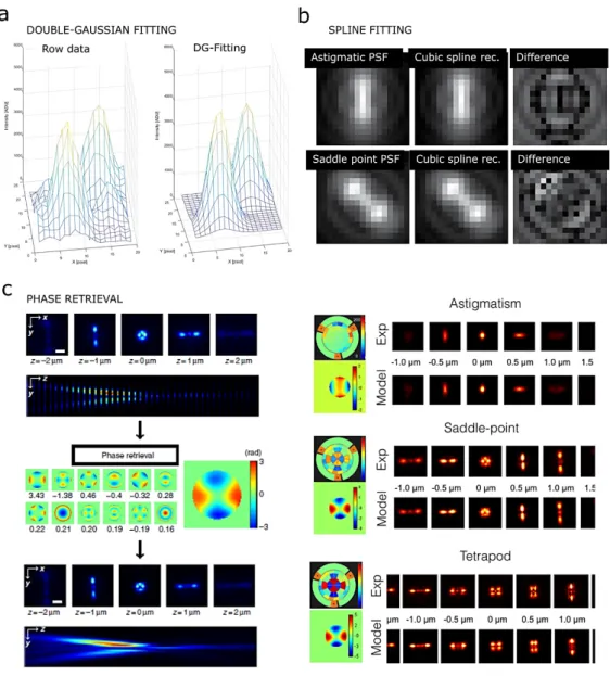
FIGURE 2-11 – DH-SMLM ALGORITHMS. 2—18
FIGURE 2-12 – DH-SMLM BEST-IN-CLASS ALGORITHM PERFORMANCE. 2—21
FIGURE 3-1 – C. CRESCENTUS CELL ENVELOPE. 3—25
FIGURE 3-2 – C. CRESCENTUS CELL CYCLE. 3—26
FIGURE 3-3 – TIME-LAPSE DUAL COLOR IMAGES OF C. CRESCENTUS. 3—26
FIGURE 3-4 – MODEL FOR CELL SIZE CONTROL AND HOMEOSTASIS IN C. CRESCENTUS. 3—27
FIGURE 3-5 – C. CRESCENTUS CELL SHAPE SCHEME. 3—29
FIGURE 3-6 – C. CRESCENTUS SHAPE IMAGES ANALYSIS. THE ANALYSIS OF 3—30
FIGURE 3-7 – C. CRESCENTUS SEPTUM SHAPE DYNAMICS. 3—32
FIGURE 3-8 – FROM 2D SMLM TO 3D DH-PSF DATA. 3—33
FIGURE 4-1 – LOCALIZATION PRECISION WITH SCMOS SPECIFIC MLE ALGORITHM. 4—36
FIGURE 5-1 – PARAMETER SPACE IN CELL SHAPE DYNAMIC STUDY. 5—43
FIGURE 5-2 – CELL SHAPE ANALYSIS PROGRAM SDADA PIPELINE. 5—45
FIGURE 5-3 – EDGE DETECTION OPTIMIZATION. 5—46
FIGURE 5-4 – POLE SIMULATOR MODEL. 5—47
FIGURE 5-5 – POLE SHAPE DYNAMICS AT THE CONSTRICTION SITE. A, AND C, 5—48
iv
FIGURE 5-7 – STORMCHASER PROGRAM PIPELINE. 5—50
FIGURE 5-8 – MOLECULE IDENTIFICATION STEP IS BASED ON CLUSTERING ALGORITHM. 5—51
FIGURE 5-9 – ARTIFICIAL DH-PSF DATASET. 5—51
FIGURE 5-10 – STORMCHASER RENDERING. 5—52
FIGURE 5-11 – 3D SMLM CHALLENGE RESULT COMPARISON. 5—54
FIGURE 5-12 – 3D SMLM CHALLENGE IMAGE RESULT. 5—55
FIGURE 6-1 – DEPENDENCE OF THE ILLUMINATION HOMOGENEITY ON THE DESIGN PARAMETERS. 6—57
FIGURE 6-2 – SCMOS ZYLA 4.3 ANDOR DARK IMAGE. 6—58
FIGURE 6-3 – SCMOS ZYLA 4.3 ANDOR READ NOISE AND GAIN DISTRIBUTION. 6—59
FIGURE 6-4 – HOT PIXELS IDENTIFICATION PROCESS. 6—60
FIGURE 6-5 – CMOS-SPECIFIC-MLE ALGORITHM AND RAPIDSTORM SOFTWARE COMPARISON. 6—62
FIGURE 6-6 – LARGE FOV STORM IMAGING OF MULTIPLE EUKARYOTIC CELLS. 6—63
FIGURE 7-1 – OPTIMIZED WAVEGUIDE DESIGN ENABLES A UNIFORM AND LARGE TIRF ILLUMINATION. 7—67
FIGURE 7-2 – LAYOUT OF THE WAVEGUIDE CHIPS FOR CLEANROOM FABRICATION. 7—68
FIGURE 7-3 – WAVEGUIDE PENETRATION DEPTH AND 1D TE0 WAVEGUIDE MODE SIMULATIONS. 7—69
FIGURE 7-4 – APPROXIMATED COUPLING EFFICIENCY ESTIMATION AND E11 WAVEGUIDE MODE PROFILE AT
THE INPUT TAPER TIP. 7—70
FIGURE 7-5 – WAVEGUIDE-PAINT PLATFORM: WAVEGUIDE-CHIP INTEGRATION IN A CUSTOM UPRIGHT
MICROSCOPE. 7—71
FIGURE 7-6 – WAVEGUIDE-PAINT IMAGING OF DNA-ORIGAMI MICROTUBULES. 7—74
FIGURE 7-7 – WAVEGUIDE-PAINT IMAGING OF COS-7 CELLS. 7—75
FIGURE 7-8 – WAVEGUIDE-PAINT IMAGING OF COS-7 CELLS. 7—76
FIGURE 7-9 – DEMONSTRATION OF WAVEGUIDE-PAINT. 7—77
FIGURE 7-10 – DIFFRACTION LIMITED AND DNA-PAINT. 7—78
FIGURE 8-1 – WORKSTATION NETWORK FOR BIG-DATA ACQUISITION AND ANALYSIS. 8—84
FIGURE 8-2 – MULTI-WELL WAVEGUIDE CHIP FABRICATION. 8—85
1—1
PART I
INTRODUCTION TO
SUPERRESOLUTION FLUORESCENCE
MICROSCOPY
1—3
1
Super-resolution principles, methods and
limitations
Fluorescence microscopy is a well-established imaging technique that allows non-invasive observation of dynamic processes within the cell, as well as probing specific proteins structure and location. During the last decades, continuous advancements were prompted by a broad, interdisciplinary effort, leading to key improvements like better labelling and increased spatial and temporal resolution. Nowadays, subcellular features can be specifically probed and resolved at a nanoscopic scale, thanks to superresolution microscopy, a set of fluorescence microscopy techniques so called for their capability to break the diffraction limit. This classical limit setting the maximum achievable spatial resolution can be described by the classical Abbe limit.
Figure 1-1 – Visualization of the imaging process. The imaging of square objects with an optical system with an impulse response described by the indicated PSF. The imaging operation, which is expressed by Equation 1, results in a blurred image of the object. The operator ∗ denotes the convolution operation.
When an ideal, dimensionless point-like object is imaged through a microscope, instead of appearing like an infinitesimal point it is actually rendered by the lens system as a blurred spot with an intensity profile defined by the response of the imaging system. Such an intensity profile is described by the point spread function (PSF) of the system. The image irradiance distribution 𝐼𝐼(𝑥𝑥,𝑦𝑦) of an extended object O(𝑥𝑥,𝑦𝑦) is thus the result of the object convolution with the system PSF:
1—4
where 𝑃𝑃𝑃𝑃𝑃𝑃(𝑥𝑥,𝑦𝑦) is the impulse response of the optical system – i.e. the image of the impulse delta-function𝛿𝛿(𝑥𝑥,𝑦𝑦). The PSF hence defines the spatial resolution limit of an optical system: the Abbe diffraction limit.
The dimensions of the PSF, 𝜎𝜎𝑃𝑃𝑃𝑃𝑃𝑃𝑥𝑥,𝑦𝑦 and 𝜎𝜎𝑃𝑃𝑃𝑃𝑃𝑃𝑧𝑧 in the lateral (𝑥𝑥 - 𝑦𝑦) and axial (𝑧𝑧) directions are in first approximation defined through the radial distance at which the value of the paraxial point spread function becomes zero:
𝜎𝜎𝑃𝑃𝑃𝑃𝑃𝑃𝑥𝑥,𝑦𝑦 ≈ 𝜆𝜆⁄2𝑁𝑁𝑁𝑁 1.2
𝜎𝜎𝑃𝑃𝑃𝑃𝑃𝑃𝑧𝑧 ≈2𝜆𝜆𝜆𝜆⁄(𝑁𝑁𝑁𝑁)2 1.3
where 𝜆𝜆 is the wavelength of the emitted light, 𝜆𝜆 is the index of refraction of the medium, and 𝑁𝑁𝑁𝑁 is the numerical aperture of the objective lens. Thus, the resolution limit for visible light (𝜆𝜆 ≈550𝜆𝜆𝑛𝑛) imaged by a high numerical aperture objective (oil immersion objective, 𝑁𝑁𝑁𝑁= 1.4 ) is 𝜎𝜎𝑃𝑃𝑃𝑃𝑃𝑃𝑥𝑥,𝑦𝑦~200𝜆𝜆𝑛𝑛 and 𝜎𝜎𝑃𝑃𝑃𝑃𝑃𝑃𝑧𝑧 > 500𝜆𝜆𝑛𝑛1. The PSF size will be more precisely described in Chapter 2.2.
Table 1-1 Super-resolution light microscopy methods. The table presents a comparison between resolution, acquisition time and image colors achievable with the super-resolution approaches used in this work. Table based on 1,2,5–8 and 9.
SIM PALM/STORM DNA-PAINT
Linear Non linear iSIM
Principle Moiré effect with structured illumination Multi-points scanning
Photoswitching and single molecule localization Binding and unbinding of fluorescently labeled oligonucleotdes Illumination
emission Linear Non linear Linear Linear Linear
Illumination excitation /Detection Wide-field CCD/CMOS Wide-field CCD/CMOS Optical iterative points scanning and deconvolution
Wide-field CCD/CMOS TIRF
CCD/CMOS
X-Y resolution 100-130nm 50nm
1.7-fold in x,y
20-40nm <20nm
Z resolution 250-350nm Not applicable <50nm (3D-STORM) spinning disk and <50nm with astigmatism
Z range 10-20 𝜇𝜇𝑛𝑛 Not described 50-100 𝜇𝜇𝑛𝑛 100nm-few 𝜇𝜇𝑛𝑛
Time resolution Milliseconds to seconds Seconds to minutes Milliseconds to seconds Minutes Several Minutes
Simultaneous
colors 3 1 3-4 2 >10
1—5
In the last decade, several different fluorescence-based approaches have been developed in order to circumvent the intrinsic diffraction limitation.
In this work, I will mainly focus on one family within the super-resolution microscopy context: single molecule localization microscopy (SMLM) and specifically on Stochastic Optical Reconstruction Microscopy (STORM)2 and DNA Points Accumulation for Imaging in Nanoscale Topography (DNA-PAINT)3. I will only briefly introduce the concept behind Structured Illumination Microscopy (SIM)4, which is a patterned excitation approach we used to image C.Crescentus bacteria with a commercial microscope. Briefly, these two super-resolution techniques offer advantages which render them attractive over other super-resolution methods. In particular, SMLM techniques offer nanoscale resolution, which surpasses achievable resolutions by all fluorescence-based techniques. SIM on the other hand allows the acquisition of fast dynamics in living cells, with high spatial resolution using a relatively low laser irradiance.
1.1
Single Molecule Localization Microscopy (SMLM)
1.1.1
SMLM with photo-switching fluorophores
Among the most commonly used methods are localization microscopies (photoactivated localization microscopy, PALM6 and stochastic optical reconstruction microscopy, STORM2). PALM and STORM are based on the photo-switchable properties of specific fluorescent molecules (fluorophores: fluorescent proteins or chemical dyes), which can be switched between a non–fluorescent (dark - OFF) state and a fluorescent (bright - ON) state by exposure to particular light wavelengths. In the case of dyes, photoswitching typically requires a reducing/oxidizing chemical buffer. Continuously acquiring images (frames) at a rate comparable with cycling the fluorophores between the OFF to an ON state makes it possible to distinguish each single fluorophores PSF within each frame. In such a way, it becomes possible to derive the actual fluorophore position from the analysis of its PSF with much better precision than analyzing the combined frames, as in widefield or even confocal microscopy (Figure 1-2).
The typical fluorophore switching rate ranges from 10 𝐻𝐻𝑧𝑧 to 1000 𝐻𝐻𝑧𝑧10, thus limits the camera exposure time between 10 𝑛𝑛𝑚𝑚 and 100 𝑛𝑛𝑚𝑚 and the total acquisition time around 20 minutes to collect about 20 thousand images necessary for a sufficient target sampling.
The PALM and STORM methods, based on fluorophore localization, yield a spatial resolution down to approximately2 20𝜆𝜆𝑛𝑛. This is due to the fact that the position 𝜇𝜇𝑥𝑥 of a single emitter can be determined to almost arbitrarily high accuracy if a sufficient number of photons generating its PSF are collected. Indeed, the localization precision of an estimation method, that assumes a Gaussian distributed PSF, can be defined in first approximation as the standard deviation of the estimated molecule location σ(𝜇𝜇𝑥𝑥) 11:
σ(𝜇𝜇𝑥𝑥) =�𝜎𝜎2(𝜇𝜇𝑥𝑥) =�𝜎𝜎𝑃𝑃𝑃𝑃𝑃𝑃2+𝑎𝑎 12⁄
𝑁𝑁 +
8𝜋𝜋𝜎𝜎𝑃𝑃𝑃𝑃𝑃𝑃4 𝑏𝑏2
𝑁𝑁2𝑎𝑎2 ~𝜎𝜎𝑃𝑃𝑃𝑃𝑃𝑃⁄√𝑁𝑁 1.4
where 𝑎𝑎2 is the pixel area, 𝑏𝑏2 is assumed background expected noise per pixel, 𝑁𝑁 is the number of expected photons and 𝜎𝜎𝑃𝑃𝑃𝑃𝑃𝑃 is the standard deviation of the point-spread function (assumed Gaussian distributed). The previous equation can be further improved by taking into account the EM gain of EMCCD cameras12 (a more accurate description is reported in Chapter 2.3):
1—6 𝜎𝜎(𝜇𝜇𝑥𝑥) =�𝜎𝜎2(𝜇𝜇𝑥𝑥) =�2𝜎𝜎𝑃𝑃𝑃𝑃𝑃𝑃 2+𝑎𝑎⁄12 𝑁𝑁 + 8𝜋𝜋𝜎𝜎𝑃𝑃𝑃𝑃𝑃𝑃4 𝑏𝑏2 𝑁𝑁2𝑎𝑎2 1.5
The localization precision is thus improved by increasing the number of emitted photons – more precisely by √𝑁𝑁 – which increases with the illumination intensity.
Figure 1-2 – Single Molecule Localization Microscopy concept. The top image represents the standard wide filed fluoresce microscopy approach: the image of a target fluorescently label is a diffraction limited image of the target. In a single molecule localization microscopy approach (bottom), the target structure of interest is labeled with photo switchable fluorophores. At the imaging start, all fluorophores are in a non-fluorescent OFF state upon irradiation with light of appropriate wavelength and intensity. A sparse subset of fluorophores is reactivated in an ON state either spontaneously or photo-induced with a second irradiation laser wavelength. The activated fluorophores, spaced further apart than the Nyquist’s limit, can be precisely localized. Repetitive activation, localization and deactivation allow a temporal separation of spatially unresolved structures in a reconstructed image.
However, the intensity of the excitation light has a limit imposed by both phototoxicity and photobleaching. Toxic effects of light primarily arise due to generation of chemically reactive species such as free radicals and specifically singlet and triplet forms of oxygen13. Reactive oxygen species react with a large variety of cellular components that can easily oxidize, such as proteins, nucleic acids and
1—7
lipids14,15 and can be critical in the mitochondria respiratory chain for DNA-damage determination16 and for directing the cell towards life or death17. These undesired reactions lead to loss of fluorescence signal (photobleaching) and physical damage to the cell or even cell death (phototoxicity).
Besides localization precision, another practical factor limits the resolution in PALM and STORM: the labeling density18. Too-low density of localizations results in an under-sampled structure, insufficient to resolve its organization19. Thus, leading to a loss of spatial information. On the other hand, if the fluorophore density is too high the images of individual fluorophores will overlap, thereby preventing each fluorophore from being localized with high precision.
Nyquist’s criterion defines in first approximation the lower limit of the labeling density: the fluorophore-to-fluorophore distance, which is the inverse of "sampling frequency", has to be at least two times smaller than the smallest sample structural feature that has to be discerned20. If 𝜌𝜌 is the density of labeling and 𝐷𝐷 is the dimension of the sample that has to be imaged, the smallest resolvable feature size thus is defined via19,21:
∆𝑛𝑛𝑦𝑦𝑛𝑛~ 2⁄𝜌𝜌1 𝐷𝐷⁄ 1.6
which is two dimensions becomes:
∆𝑛𝑛𝑦𝑦𝑛𝑛~ 1⁄�𝜌𝜌 1.7
Therefore, to achieve 10-nanometer resolution, molecules must be spaced a minimum of 5 nanometers apart in each dimension to yield a minimum density of 4 × 10⁴ molecules per square micrometer. This means, that in a diffraction-limited region of 250-nanometers in diameter (about 0.05 square micrometer) there should be about 2000 molecules to achieve 10-nanometer resolution. Since only one of these fluorophores should reside in its fluorescent state per cycle, the lifetime of the OFF state (𝜏𝜏𝑂𝑂𝑃𝑃𝑃𝑃) has to be 2000 times longer than the lifetime of the fluorescent ON state (𝜏𝜏𝑂𝑂𝑁𝑁). 𝜏𝜏𝑂𝑂𝑃𝑃𝑃𝑃 has been reported to vary from 10 to 100 𝑛𝑛𝑚𝑚 to several seconds10. The lifetime of the ON state depends both on the fluorescence lifetime (the average time the molecule stays in its excited state before emitting a photon) and the number of times the molecule can cycle between its singlet ground state and the excited state before undergoing stochastically in the OFF state. Typical fluorescence lifetimes are within the range of 0.5 to 20 nanoseconds and the molecule can emit a photon about 1000 times before switching OFF. Therefore, the total time 𝜏𝜏𝑂𝑂𝑁𝑁 a molecule can stay in the ON state is of few milliseconds at most.
Fluorophores with a higher 𝜏𝜏𝑂𝑂𝑃𝑃𝑃𝑃/𝜏𝜏𝑂𝑂𝑁𝑁 ratio allow the sample to be labeled with higher density since the risk of false localizations caused by the overlapping of multiple fluorophore signals within the same diffraction-limited area, is lower. On the other hand, high photoswitching ratios result in a small number of localizations per image and thus prolong the acquisition time unnecessarily.
However, it is important to underline that the argument concerning the resolution link to label density is only true in a first approximation. Indeed, resolution also depends strongly on the underling sample structure, the presence of not uniform background and localization precision and can therefore be better described by the following expression22,23:
∆𝑛𝑛𝑦𝑦𝑛𝑛~ 1⁄�𝑙𝑙𝑙𝑙𝑙𝑙 𝜌𝜌 1.8
Today, fluorophores have become highly optimized in their targeting, photostability, and photoswitching24–26 to make it possible to routinely resolve structures down to the nanometric scale.
1—8
1.1.2
3D SMLM approaches
Cells and their intra-cellular structures and organelles are fundamentally three-dimensional. For this reason, many efforts have been employed to access the third spatial dimension and to improve axial resolution. As previously mentioned, this work focuses mainly on the SMLM family. However, I will briefly compare the advantages and disadvantages of the SMLM approach with SIM: another approach we could easily access at EPFL through a commercially available microscope.
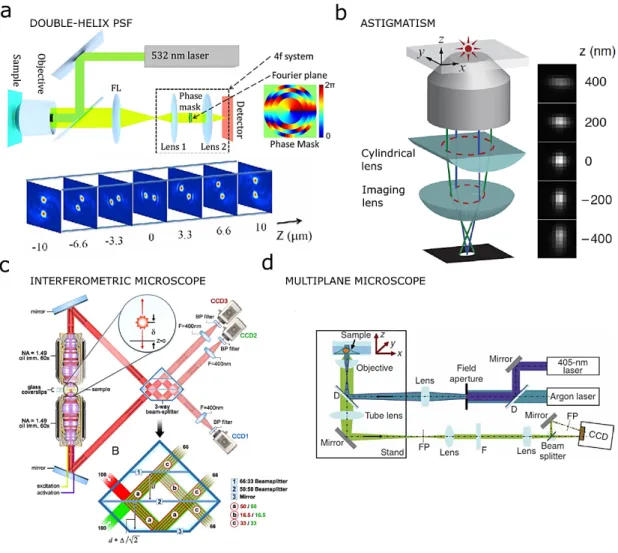
Figure 1-3 – 3D SMLM approaches. a, Typical DH-PSF of a conventional wide-field microscope at different axial planes37
(top); The phase mask is mounted in the Fourier plane, which is the center plane between Lens 1 and Lens 2 forming a 4f system. The phase mask is typically made of positive photo-resist (AZ-4210, Clariant) spin-coated on a glass slide with different thicknesses to generate different phase delays38. The simulated phase mask pattern shown approximates the double helix
phase mask reported in 30; b, Optical diagram to produce the desired astigmatic aberration of the PSF by introducing a
cylindrical lens into the imaging path. The z coordinate is extracted from the ellipticity of its image. The right panel shows images of a fluorophore at various z positions29; c, Schematics of an single-photon fluorescence interferometric microscope.
A point source emits a single photon both upwards and downwards. The single photon interferes in a special 3-way beam splitter. Since, the difference in path lengths of the upper and lower beams directly depends on the axial position of the source, the axial position of the source molecule can be determined from the relative amplitudes of the source images from the 3 cameras31; d, Optical diagram of a multiplane microscope implemented into a conventional microscope for wide-field.
Emission fluorescence is split into two paths to create two separate image planes on the same CCD camera32.
Linear SIM has provided ~100 𝜆𝜆𝑛𝑛 lateral and ~300 𝜆𝜆𝑛𝑛 axial resolution in the mammalian nucleus 27, while non-linear SIM has so far only been demonstrated in two dimensions28.
With single molecule microscopy techniques such as PALM/STORM, it is possible to simultaneously achieve higher lateral (around ~25 𝜆𝜆𝑛𝑛) and axial resolution (around ~50 𝜆𝜆𝑛𝑛)1. However, current 3D
1—9
PALM/STORM are limited to a maximal depth range of 100 𝜆𝜆𝑛𝑛 − 𝑓𝑓𝑓𝑓𝑓𝑓𝜇𝜇𝑛𝑛 whereas 3D SIM has an axial range of 10 𝜇𝜇𝑛𝑛 −20 𝜇𝜇𝑛𝑛8.
For application where 3D resolution weight more than imaging depth, 3D SM approaches are the methods of choice. Different techniques have been developed for far-field SM localization microscopy based on the PSF engineering (such as astigmatic imaging29 and double-helix (DH) PSF30), interferometry (such as iPALM- where the axial position is calculated from single photon interference between opposing objectives31) and multiplane imaging32. In the multiplane approach, the axial information is extracted from the simultaneous measurement of the PSF shape at different focal planes. Multiplane provides 3D imaging over a depth of less than one micron without axial scanning at a resolution of 30 nm laterally and 80 nm axially and over several micron with axial scanning32. However, this approach requires either the use of two cameras, which introduces synchronization and cost drawbacks, or the binning of one camera, which limits the field of view. While extremely precise31 – its achievable axial resolution is 10-20 nm – the interferometric approach is not yet widely adopted. This is most likely due to the ease of adopting 3D capability by commercial engineered PSF or adding a simple lens to existing standard microscopes whereas an upgrade to iPALM requires extensive modification. The realization of a 3D single molecule platform based on the introduction of commercial engineered PSF or a lens, is easier to achieve with respect to the interferometric PALM technique which requires extensive modifications of a standard microscope33 (see Figure 1-3). Additionally, the PSF engineering approach has a longer depth range with respect to pure interferometry. In fact, in the interferometric system the maximum depth is about 200 𝜆𝜆𝑛𝑛31, while the astigmatic and DH-PSF approaches provide a depth of field of about 600 𝜆𝜆𝑛𝑛34 and 2−3𝜇𝜇𝑛𝑛33,35 respectively.
All together, a DH-PSF microscope is the technique that allows one to achieve the best axial localization precision (up to 20 𝜆𝜆𝑛𝑛) and lateral localization precision (10 𝜆𝜆𝑛𝑛) over an axial range larger than 2 𝜇𝜇𝑛𝑛30. The DH method is based on an engineered phase mask that, when added to a conventional widefield microscope, enables the generation of a PSF that changes with focus depth. The PSF generated by this mask appears as two bright lobes which revolve around one another as a function of 𝑧𝑧-axial position36 (Figure 1-3 a and Figure 1-4).
Figure 1-4 – 3D-PSF simulated dataset . Summary of different simulated datasets. Each dataset is characterized by its structure (endoplasmic reticulum (ER) or microtubules (MT)), by its modality (two dimensional (2D), astigmatic (AS), double helix (DH), biplane (BP)), its density (low density (LD) or high density (HD) and by its SNR determined by the level of noise. Figure taken from 39.
1—10
The angle of the axis connecting the center of the two lobes relative to a fixed reference axis, will encode the 𝑧𝑧 position. The center of the midpoint between these two centers yields the lateral position of the fluorophore (Figure 1-3 a). A current limitation of this approach is set by the overall large size occupied by the two lobes of the PSF distribution. At high molecule density, DH-PSFs tend to overlap more frequently affecting the SNR and localization precision. Thus, the improved axial resolution and extended range introduced by DH-PSF engineering comes at the cost of limiting the experimental acquisition to low molecule density conditions.
1.1.3
DNA Points Accumulation for Imaging in Nanoscale Topography (DNA-PAINT)
“Points Accumulation In Nanoscale Topography” (PAINT)40 provides several improvements over the above mentioned SMLM techniques such as precise and quantitative multiplexed imaging capability for in vitro or in situ experiments3,41–44. It combines multi-pseudocolor (more than ten tones) imaging with optimal localization precision and specificity3. Unlike other stochastic super-resolution methods, DNA-PAINT employs non-photoswitching fluorophores which do not blink between different fluorescence states. Instead, it leverages on the stochastic binding and unbinding of fluorescently labeled oligonucleotides ("imager" strands) in DNA-PAINT3,42 and protein-fragment probes in ‘integrating exchangeable single-molecule localization’ (IRIS)45 to obtain the same blinking effect.
Figure 1-5 – DNA-PAINT sample scheme. Cell antibodies are chemically modified to become DNA-conjugated antibodies and used for in situ DNA-PAINT imaging of fixed cells (Left). DNA origami nanostructures can be easily seeded on BSA/biotin/streptavidin-coated surface for in vitro experiments (Right)44.
The sampling of the target sites with imager strands that are continually replaced, provides an effective solution to photobleaching, which limits standard fluorescence imaging approaches. Moreover, tagging the target with diverse docking strands and probing them with their respective complementary imager strands, enables sequential pseudo-color imaging with unlimited multiplexing. DNA-PAINT offers the possibility to perform in situ imaging of fixed cells or in vitro imaging of DNA-origami structures (Figure 1-5).
The in situ protein-labeling strategy is based on immunostaining with DNA-conjugate primary-secondary antibodies, where the antibodies are chemically modified to link the DNA-docking strand to the secondary antibody.
1—11
In vitro DNA origami structures provide a framework to test a fluorescence microscopy method by placing defined numbers of small molecules at nano-metric distances in a programmed way as distinct calibration marks43.
DNA origami structures are created by folding a long single strain DNA molecule named ‘scaffold-strand’. The folding process is set by the specific binding of hundreds of short synthetic oligonucleotides (‘staple-strands’) to precise predefined regions on the scaffold46,47 (Figure 1-6). To allow DNA-PAINT imaging, the staple strands of the DNA-origami structure are usually extended by adding single-stranded docking sites that can bind to the imager strands41.
Figure 1-6 – DNA-ORIGAMI creation principle.DNA-nanoshapes are mainly made by a long DNA-scaffold strand. The scaffold strand is bent using DNA-staple strand placed at the designed corresponding scaffold-strand sites. The origami has exactly the size and shape design and can thus be used as a caliber to measure other unknown structures.
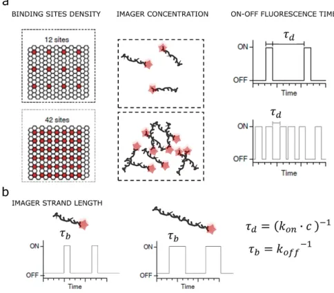
The sample and experiment design of both in situ and in vitro experiments can strongly affect the resulting performance of the experiment (such as achievable spatial and temporal resolution – see Figure 1-7). For example, when decreasing the site distance or increasing the imager strand concertation, the dark time 𝜏𝜏𝑑𝑑 (inter-event lifetime) decreases, which leads on one hand to a lower total
imaging time but on the other hand to a higher probability of SM-PSF overlapping and hence lower localization precision. The following expression defines through 𝜏𝜏d, the necessary time to have at least
one binding event with a probability higher than 98%: 𝑃𝑃(1 𝑏𝑏𝑏𝑏𝜆𝜆𝑑𝑑𝑏𝑏𝜆𝜆𝑙𝑙𝑏𝑏𝜆𝜆∆𝑡𝑡) =� 1𝜏𝜏 𝑓𝑓−𝑡𝑡𝜏𝜏𝑑𝑑𝑡𝑡= 1− 𝑓𝑓−∆𝑡𝑡𝜏𝜏 ∆𝑡𝑡 0 > 98% 1.9 ∆𝑡𝑡>𝑙𝑙𝜆𝜆( 1 −0.98)−1∙ 𝜏𝜏 𝑑𝑑 ∆𝑡𝑡> 4∙ 𝜏𝜏𝑑𝑑
Since 𝜏𝜏𝑑𝑑= (𝑘𝑘𝑜𝑜𝑛𝑛∙ 𝑐𝑐)−1 where 𝑐𝑐 is the imager strand concentration (typically about 1-10 nM), and 𝑘𝑘𝑜𝑜𝑛𝑛 the probe association rate (typically of 106 Ms−1) the necessary waiting time for at least one binding event is about 100-1000s and a total imaging time of 400-4000s (10-60 minutes).
Another important parameter is the binding time 𝜏𝜏𝑏𝑏 (or the dissociation rate 1/𝜏𝜏𝑏𝑏) which
1—12
design and estimation of such parameters determine the signal to noise (SNR) and the camera exposure time. Increasing the imager strand length increases the number of photons generated during one single binding event. However, this increase in Signal to Noise Ratio (SNR) comes at the expense of exposure time required to image a sample.
A major advantage of PAINT is that fluorophores in solution can iteratively sample the structures of interest48, in a process that is only limited by the patience of the experimentalist49. Other advantages include the unlimited multiplexing of EXCHANGE-PAINT for multicolor imaging3 and the possibility to quantify the number of binding sites at each location using qPAINT50.
Figure 1-7 – DNA-PAINT experimental parameters affecting the imaging performances. a, The site density or the imager concentration affect the dark time 𝜏𝜏𝑑𝑑 (inter-event lifetime) and thus the total imaging time. b, The imager strand length affects
the signal to noise but also the necessary camera exposure time. Figure inspired by 44.
To allow binding and dissociation, PAINT requires a reservoir of fluorescent probes (e.g. labelled DNA oligos) in solution surrounding the sample, which brings its own limitations to the method. First, it requires axial optical sectioning to reject the background signal from fluorophores in solution. This can be mitigated in the case of fluorescence enhancement upon binding as for fluorogenic dyes40, quenching of unbound probes51 or Förster resonance energy transfer-(FRET) PAINT52,53. However, these approaches come at the cost of reduced labeling flexibility, increased sample preparation complexity and a potential reduction in localization precision54,55.
Although DNA-PAINT offers several advantages such as continuous replacement of possible bleached molecules, as well as high localization signal and large fluorophores pool availability, it presents two main challenges for the imaging system.
First, DNA-PAINT requires an optical sectioning illumination to minimize the background signal from the unbound imager strands. The most common way to realize such an illumination is either through objective-based Total Internal Reflection Fluorescence (TIRF) technique or light sheet illumination (Figure 1-8). However, both these two approaches are limited either in FOV size or uniformity. We will investigate the limitations of these approaches more deeply in the next Chapter 2.1.
1—13
A second DNA-PAINT limitation is set by the trade-off between binding duration and localization precision. To improve the localization precision, the most effective way is increasing strand length – and thus binding duration. This increases the number of photons generated during one single binding event. But the elevated Signal to Noise Ratio (SNR) comes at the expense of exposure time required to image a sample, which is typically ten times higher than other localization-based microscopy methods, such as PALM or STORM (a few hundred milliseconds instead of ten milliseconds)44.
Figure 1-8 – Optical sectioning can be obtained by light sheet or TIRF approaches. DNA-PAINT requires optical sectioning to suppress the background generated by the fluorophore in solution. This can be obtained either with light sheet or TIRF microscopy.
Using waveguide-based evanescent field systems instead of the standard TIRF configuration for DNA PAINT microscopy, has several advantages. First, a waveguide illumination separates the excitation light from the fluorescence emission path, making it possible to achieve a uniform and large excitation field target, and to optimize the objective for the sole imaging purpose.
The larger excitation field leads to more sample being exposed within one FOV. Total data throughput is thus increased and acquisition times reduced. Furthermore, evanescent field illumination offers greater freedom in customizing the chip design to better fit the set up where it will be integrated. Although waveguide evanescence field illumination has been tested in fluorescence microscopy56–59 and in superresolution microscopy60, applying this solution to DNA PAINT imaging requires an apparatus capable to produce the required evanescent field, combined with a fast buffer exchange, with a specific design for the waveguide-chip and the microscope integration. We present in Chapter 4.2, an illumination field of uniform evanescent light, a flexible waveguide-based platform that provides a large and uniform evanescent excitation over a 100 × 2000 µm2 area.
1.2
Structured illumination microscopy (SIM)
In the context of super-resolution, Structured Illumination Microscopy (SIM) is a wide-field microscopy technique which utilizes the projection of a known illumination pattern (often sinusoidal grids) onto the sample to extract higher resolution information4,61. In a diffraction limited microscope, the observable spatial frequencies in the sample define a circular region of radius 𝑘𝑘0~ 2𝑁𝑁𝑁𝑁 𝜆𝜆⁄ in the Fourier space (Figure 1-9, a) set by the diffraction limit of light. But, if the excitation light is modulated
1—14
by a spatial frequency 𝑘𝑘1, such as a sinusoidal pattern, previously unobservable information – containing frequencies from outside of the observable region – becomes encoded in the form of Moiré fringes. By recombining multiple images in Fourier space with different pattern positions and orientations, a super-resolved image is obtained with the maximum detectable spatial frequency increased to 𝑘𝑘0+𝑘𝑘1 (Figure 1-9, b) 4,61.
Figure 1-9 – Structured-illumination concept. (a) The set of sample spatial frequencies that can be observed by the conventional microscope defines a circular observable region of radius 𝒌𝒌𝟎𝟎 in frequency space. (b) If the excitation light
contains a spatial frequency 𝒌𝒌𝟏𝟏, a new set of information becomes visible in the form of Moiré fringes (hatched circle). This
region has the same shape as the normal observable region but is centered at 𝒌𝒌𝟏𝟏. The maximum spatial frequency that can
be detected (in this direction) is 𝒌𝒌𝟎𝟎+𝒌𝒌𝟏𝟏62.
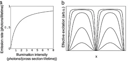
Since the projection of the illumination pattern itself is limited by the diffraction of light, the resolution limit can be extended by a factor 2 at most in the linear case. However, if the sample’s fluorescence emission is non-linearly dependent on the illumination pattern intensity, such as in a saturated regime (Saturated Structured Illumination Microscopy – SSIM), the emission pattern could in principle contain arbitrarily higher spatial frequencies than the illumination pattern itself62. This particular nonlinear phenomenon is due to the non-instantaneous photon emission process of an excited fluorophore. After photon absorption, the fluorophore needs an average time (the fluorescence lifetime) to relax back to the ground state with a photon emission. Therefore, it cannot respond linearly to the illumination intensities above one photon per absorption cross section per lifetime.
Figure 1-10 – Nonlinear fluorescence emission introduces high frequency harmonics. Figure (a) shows the nonlinear dependence of the fluorescent emission rate on the illumination intensity in the saturation regime. (b) The emission pattern resulting from sinusoidal patterned illumination with different peak pulse energy densities (from the bottom to top curve 0.25, 1, 4, 16, and 64 times the saturation threshold) 62.
1—15
If a sample is illuminated with a sinusoidal light pattern that has a light intensity above this threshold, the emission rate per fluorophore thus has a pattern with a nonsinusoidal shape (Figure 1-10). This pattern of emission contains higher spatial frequencies than the illumination pattern itself. Unfortunately, saturation requires extremely high light intensities that are likely to accelerate photobleaching and photodamage, making this implementation non suitable for studies of living cells.
However, another nonlinear SIM approach was later implemented by exploiting the optical photoswitching property of select fluorophores such as Dronpa fluorescent protein63 to provide the required nonlinearity. Photoswitchable fluorescent molecules can be reversibly switched between a fluorescent ON state and nonfluorescent OFF state using light with two different wavelengths. Saturating either of these population states results in a nonlinear relationship between the fluorescence emission and the illumination intensity. In this case, the required intensity is six orders of magnitude lower than the one necessary in the traditional saturated SIM63. Thanks to this principle, a resolution of <50𝜆𝜆𝑛𝑛 has been achieved with non-linear SIM on purified microtubules labeled with the fluorescent photoswitchable protein Dronpa63.
2—1
2
Image quality limitations in SMLM
The resolution, uniformity and size of a final reconstructed SMLM image is affected by several factors:
• the sample preparation (e.g. label density64 and other general properties of a fluorescent molecule such as ON-OFF possible kinetics, duty cycle and photon budget65)
• the sample illumination
• the fluorescence detection process (e.g quantum efficiency66 of the setup, camera critical parameters such as quantum efficiency, read noise and speed, duration of the acquisition, background),
• the molecule localization and super-resolved image rendering processes36 (i.e. the adopted localization algorithm)
We previously focus on the implication of the label density (i) on the image reconstruction quality. In this Chapter, we will discuss why the sample illumination (ii) quality is critical for SMLM image quality and the main approaches adopted to address the current challenges. We will also explore the advantages and disadvantages of different localization algorithms (iv). Further (Chapter 4.1), we will investigate the critical camera aspects setting the limit to the molecules detection process (iii).
2.1
Illumination aspects critical for image quality
Sample illumination is particularly critical in SMLM where the single molecule (SM) sampling uniformity and localization precision define the achievable super-resolved image resolution and quality. Indeed, intensity, background and uniformity of the illumination approach set the SMs density per frame (through the activation or photo-switching rate illumination intensity5) and their signal to noise and thus the continuity of the target sampling and the SM position estimation accuracy.
In this chapter, we will explore the possible factors that strongly influence and limit the sample illumination qualities such as the global and local spatial dependence of the illumination field resulting from a Gaussian beam and from the interference of coherent light respectively. Moreover, we will compare different illumination approaches adopted to reduce out of focus fluorescence background that arises from a standard epi-illumination.
Focusing an excitation beam at the objective’s back focal plane produces a wide-field illumination with an illumination spot size proportional to the objective’s numerical aperture (NA). Since the irradiance distribution of the input beam at the back focal aperture is typically Gaussian, the resulting illumination spot will present an intensity drop moving from its center to the periphery.
This aspect leads to different limitations. The irradiance inhomogeneity compromises the localization precision across the FOV and forces either to limit the final image to the central part of the FOV, where the irradiance meets the requirement for doing SMLM (1–10 kW cm−2 for STORM and PALM)66,67, or to image over a longer acquisition time than the one achievable by flattening the same irradiance. When the irradiance is too high, the emitter density per frame is low and the acquisition time to sample all the possible labelled sites becomes long. On the other hand, where the irradiance is too low, the molecule density per frame is high and with low signal. The result can be both the production of artifacts and a
2—2
lower resolution. The illumination uniformity is therefore fundamental for the optimization of the quality, time and size of a SMLM imaging process.
2.1.1
Global field flattening with Köhler integrator or beam shaping elements
The Köhler integrator68,69 has been previously adopted to address this need. Our work presents a straightforward integration and extension of this solution in a SMLM CMOS-based microscope70. A Köhler integrator is a combination of multiple parallel Köhler illumination systems, typically realized with microlens arrays, which minimizes both the spatial and angular dependence of the light source irradiance.
Figure 2-1 – A Kohler integrator. A Kohler integrator system provides a flat field and homogenous illumination independent of angular field and shape of the light source. A simple Köhler illumination system (left-top panel) illuminates each point at the target area with every emitter point at different positions across the source so that the spatial irradiance variations across the source are averaged out at the target illumination. However, this simple configuration cannot account for intensity variations of light source that generates a high directed beam (left-bottom panel). In a Köhler integrator, the light from the source is collected by an array of lenses to account for both angular and spatial inhomogeneity.
As shown in Figure 2-1, a simple Köhler illumination can only average out the irradiance spatial variations by overlapping an image of each light source point at each point of the target illumination area. This is achieved by simply focusing the light at the back focal aperture of the imaging objective.
However, in the presence of high directional source, which emits a stronger signal at a certain angle acceptance compared to another angle range (such as lasers used in SMLM imaging), a simple Köhler illumination will project every angle range always at the same position producing a spatial irradiance inhomogeneity.
A micro-lens-array-based (MLA) Köhler integrator addresses this problem by using a micro-lens-array comprised of lenses placed at different positions around the optical axis, with each collecting ray bundles coming out from the source at different angles. The rays coming out from the source at different angles will therefore overlap at every point in the resulting illumination area, averaging out any angular dependence of the source. A system with two MLA (Figure 2-3 b), where the second MLA is placed at one focal length after the first, will further improve the illumination thanks to the lenslets in the second MLA which cancel the quadratic phase curvature imparted by the first MLA71.
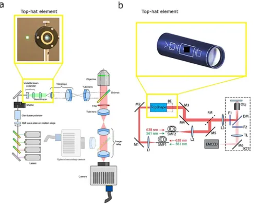
An alternative approach for achieving a so called ‘top-hat’ illumination profile has been demonstrated with both diffractive and refractive beam shaping elements72–74. Single low-cost
2—3
refractive beam-shaping element are commercially available and can be easily placed in any PALM/STORM microscope.
Figure 2-2 – Flat-field illumination employing beam shaper diffractive elements. a, The laser beams passing through the beam-shaper element emerges with a top-hat profile which is imaged onto the sample via a telescope and reflection off a dichroic mirror73. b, The laser beams are coupled into two single mode fibers. One output fiber beam is collimated and passes
through the beam-shaper element producing a top-hat profile74.
2.1.2
Local speckles and interference fringes homogenization
The free space excitation laser light along the optical path undergoes scattering and diffraction at the mirrors, lenses and coverslip surfaces. The production of mutually coherent sources, with different phase at every surface, generates interference fringes that vary with sample position and composition and with any optical component micro-position displacement. These unpredictable patterns produce non-uniformities in the sample illumination eventually giving rise to artifacts.
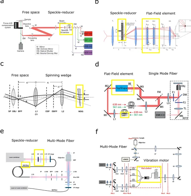
To degrade the spatial coherence of the beam and to reduce the illumination in-homogeneity a spinning diffuser is typically adopted70,75 (Figure 2-3 a and b). However, this approach eliminates only the speckles and fringes due to imperfections in the optical system. To also remove the fringes arising from sample irregularities itself, the excitation beam should illuminate the sample from different directions. Radial scanning with an off-axis focused beam the back focal plane of the microscope objective, produces a collimated beam incident on the sample with a constant polar angle β (lower than 90°) and a rotating azimuthal angles (Figure 2-3 c). This solution can be implemented by using either an optic, such as galvomirrors, or a spinning wedge76.
Another approach for achieving a homogenous excitation field employs optical multi-mode or single mode fiber. Single mode fiber generate a homogenous excitation field but with a global not-flat irradiance that requires an extra beam-shaper element for profile flattening74 (Figure 2-3 d). On the other hand, multimode optical fibers generates a flat field with intensity fringes due to the modes interference. Mode scramblers are commercially available and they can be easily adopted75,77 (Figure 2-3 e). However, the speckle-reducer results in significant loss of total laser power. An efficient mode scrambling can be achieved through a more sophisticated setup using either a multi-length optical fiber
2—4
bundle78 or a high-frequency vibration motor79 (Figure 2-3 f). These methods are not limited by the speed of the wedge, mirror, diffuser or speckle-reducer and they do not involve the transmission through extra optical component and thus enabling low-power losses and high-speed imaging.
In the next Chapter, we will discuss which of these approaches can be compatible with a total internal reflection TIRF illumination and their limitations.
Figure 2-3 – Speckles and interference fringes homogenization approaches. . a and b, The spatial coherence of the beam can be degraded by introducing in the free space optical path a spinning diffuser that reduces the illumination in-homogeneity70,75. a, Scheme of the optical arrangement of a PALM/STORM apparatus build around an Olympus IX-71 inverted
fluorescence microscope where a speckle scrambler is placed on the intermediate focal plane of a Keplerian beam expander75. b, The spinning diffuser element can be easily integrated in a Koehler integrator system and its position (Δr) determines the
extended source size. f1, fc and fOBJ, are the focal lengths of corresponding thin lenses; DMLA, DBFP, aperture sizes; MLAs
micro-lens arrays with identical fical length fMLA70. c and d, An uniform excitation can be produced by temporally and spatially varying the input beam using a spinning wedge or shaping the input beam with a diffractive optical element. Both these two approaches are compatible with a TIRF illumination because they do not degraded the coherence of the input beam that would make it hard to focus the beam at the back focal aperture of the objective. c, A spinning wedge diverts the beam into a hollow cone and the following lenses converge the collimated beam into a focused spot that traces a circle at the objective’s back focal plane. When the wedge is spun rapidly, the different interference patterns are averaged out over a single camera exposure. SP, sample plane; OBJ, objective; BFP, back focal plane of the objective; L1, lens 1; ESP, equivalent sample plane as formed by L1; EBFP, equivalent back focal plane as formed by L1; L2, lens 2; WDG, spinning wedge76.
2—5
d, Imaging system was constructed with an Olympus IX73 inverted microscope where the laser sources were coupled into two single mode fibers. One output beam from a single-mode fiber was collimated with an achromatic lens and sent to the beam shaper (TopShape, asphericon GmbH).BE, 1.5x beam expander; DM, dichroic mirror; F1-2, excitation/emission filters; FM, flip mirror; L1-3, lenses; M1-6, mirrors; Obj, objective; SMF1-2, single mode fibers; TL, tube lens.74.e, and f, Multi-mode fibers are employed to achieved a flat field illumination in combination with a speckle reducer (e) and a vibration motor (f).
e, Free-space propagating lasers are focused on the speckle-reducer before coupling into a multimode fiber. The fiber is coiled to further mix the laser modes. The image of the fiber output is then formed into the sample by relay lenses. The second optical path, is designed to perform standard TIRF illumination by focusing the light on the back-focal plane of the objective. Lxx: achromatic lens with focal length of xx mm, SR: speckle-reducer, MM: multimode, SM: single-mode, IP: image plane, BFP: back-focal plane, M: mirror and DM: dichroic mirror77. f, A uniform and flat field illumination is achieved by employing a
multi-mode fiber combiner realized to reduce the speckle pattern contrast79. The optical setup for quantifying the
illumination homogeneity at the sample plane. M1-M7: mirrors; Iris1-Iris4: Iris diaphragms; L1/L2: Fiber coupler with a focusing lens; L3: Microscope objective (10 × /NA0.25, Olympus); L4: Achromatic doublet lens; L5: Achromatic doublet; L6: Achromatic doublet lens; L7: Achromatic doublet lens; TL: Tube lens; Objective: Water-immersion microscope objective (60XW/NA1.2, Olympus); DM: Dichroic mirror; F: Emission filter.
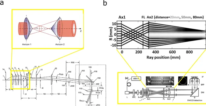
Figure 2-4 – Flat-field TIRF illumination using axicon lens. a, A collimated beam is generated by placing the light source (1) at the focal point of a lens-2 with focal length f2. A mask (3) is used to block the center portion of the beam that could produce scattering from the imperfection of the axicon lens center. Another lens (4) of focal length f4, focuses the light to a point in an image plane while the first stationary axicon lens (5) placed between these two lens (1 and 2) shifts the direction of the converging beam in a radial outward direction. The second axicon (6) shifts further outward the converging beam emerging from lens 2 and converging on the image plane (8) where it creates an annular illumination of a radius set by the distance x6 which increases linearly with x6. The disk of light is then collimated and relayed from the image plane (8) to the back pupil plane of the objective (909), by anther lens (20), the tube lens (905) and the objective (910). Figure taken from80.
Magnified view of the axicon lens principle taken from 81. b, Main optical components of another TIRF setup realized with
two axicons (Ax1 and Ax2) lens, laser (L), radial polarization converter (RPC), beam expander (BE), focus lens (FL), and a dichroic mirror (DM). A disk of light is focused on the objective back focal (BFP) to produce a TIRF illumination at image plane (IP)82.
2—6
2.2
Optical sectioning techniques
The quality of the imaging process does not depend only on the sample illumination uniformity. The viability of the biological sample is also crucial for obtaining meaningful and reliable biological results. Thus, many efforts have been done to find a strategy to minimize unnecessary dose of light delivery. A straightforward solution is to illuminate the sample target with a thin layer of light to avoid the excitation of the surrounding area. An optical sectioning approach has the advantage, not only to minimize the phototoxicity, but also to decrease the background and thus to improve the single molecule SNR.
Optical sectioning can be provided by light sheet83, highly inclined and laminated optical sheet (HILO)84, confocal rejection85 or total internal reflection fluorescence (TIRF)41. However, confocal rejection also reduces the number of detected signal photons, while light sheet, HILO or objective TIRF are typically limited in both size and uniformity of illumination (Figure 2-5).
I previously described sophisticated setups using scanning of the coherent excitation light, such as the one based on a spinning wedge to rotate the beam86,87 (Figure 2-3 c), to homogenize speckle pattern. These approaches are compatible with an objective-TIRF illumination and can reduce interference patterns, but they do not eliminate the spatial dependence of the field resulting from a focused Gaussian beam.
Figure 2-5 – Objective TIRF limitations.Objective TIRF illumination suffers of global and local in homogeneities.
Another elegant approach is based on axicon lens80,82,88 (Figure 2-4) to produce a small annular illumination at the objective back focal aperture suitable for objective-TIRF illumination and on a moving diffuser to spatially and temporally vary the excitation beam to eliminate the effects of laser speckle and interference fringes. This approach results in very low light loss compared to a much larger loss from the annular aperture and in a uniform TIRF illumination. However, the achievable field-of-view (FOV) is limited by the objective lens.
Other flat-field illumination methods that are easy to implement but not compatible with TIRF illumination are the previously described approaches based on multimode fiber combined with a speckle reducer77,79,89 (Figure 2-3 b, e and f). In fact, they rely on the loss of the beam spatial coherence which prevents tight focusing of the beam at the back focal plane of the objective for TIRF illumination.
More recently, an effective flat-field objective-TIRF illumination has been proven by employing commercial beam shaper elements74(Figure 2-3 d). However, also this approach presents a limited uniformity and achievable field-of-view (FOV) size set by sample uniformity and the objective NA respectively.
2—7
A waveguide-TIRF approach provides a flat thin excitation field as large as the waveguide surface with an optical configuration that decouple the excitation light path from the detection path and thereby decreasing unwanted excitation light in the detection path and letting a free choice of the imaging objective.
In the next chapter, we will discuss when a light sheet or HILO illumination is more suitable and the main advantages and disadvantages of a waveguide TIRF approach.
2.2.1
TIRF illumination
Total internal reflection fluorescence (TIRF) microscopy relies on the evanescent field generated by the light that undergoes total internal reflection at the interface between coverslip and the sample90. The decay length 𝑑𝑑 of the evanescent field intensity I sets the optical sectioning thickness and can be tuned by properly setting the incident beam angle 𝜃𝜃, the beam wavelength 𝜆𝜆 and the difference (𝜆𝜆𝑐𝑐𝑐𝑐− 𝜆𝜆𝑐𝑐) between the sample holder (coverslip) and sample refractive indices:
𝐼𝐼 =𝐼𝐼0𝑓𝑓−𝑧𝑧/𝑑𝑑 2.1
𝑑𝑑=4𝜆𝜆𝜋𝜋 1
�𝜆𝜆𝑐𝑐𝑐𝑐2𝑚𝑚𝑏𝑏𝜆𝜆2𝜃𝜃 − 𝜆𝜆𝑐𝑐2
2.2
Figure 2-6 – Prism-TIRF and objective-TIRF configurations. Simplified sketch of the working TIRF principle for prism and objective TIRF approaches: the beam hits the sample-coverslip interface at an angle higher than the critical angle producing an evanescent field for sample excitation.
TIRF illumination typically generates a thin excitation field of about 200 nm just above the sample glass surface (Figure 2-6) making it suitable to efficiently detect, localize and track molecule events near the cell plasma membrane. Because of its uniquely thin selective illumination, only targeted fluorophores near the sample-glass interface are excited leading to less phototoxicity for the cell and higher signal to noise (2000 fold less background91) compared to standard wide field epi-illumination prone to out of focus fluorescence signal.
There are different configurations for producing a TIRF illumination commonly named objective-TIRF90, prism-TIRF91,92 and waveguide-TIRF57 depending on the strategy used to produce the reflection of the excitation beam at the glass-aqueous solution interface. In a standard objective-TIRF approach, the same imaging lens is also used to cast an off-axis light beam such that it undergoes total internal reflection at the coverslip-sample interface. This ensures that only the resulting evanescent light field