ADEMU WORKING PAPER SERIES
Sovereign Default in a Monetary Union
Sergio de Ferra † Federica RomeiŤ May 2018 WP 2018/118 www.ademu-project.eu/publications/working-papers Abstract
In the aftermath of the global _nancial crisis, sovereign default risk and the zero lower bound have limited the ability of policy-makers in the European monetary union to achieve their stabilization objective. This paper investigates the interaction between sovereign default risk and the conduct of monetary policy, when borrowers can act strategically and they share with their lenders a single currency in a monetary union. We address this question in an endogenous sovereign default model of heterogeneous countries in a monetary union, where the monetary authority may be constrained by the zero lower bound. We uncover three main results. First, in normal times, debtors have a stronger incentive to default to induce more expansionary monetary policy. Second, the zero lower bound, or constraints on monetary policy may act as a disciplining device to enforce repayment of sovereign debt. Third, sovereign default risk induces countries with a preference for tight monetary policy to accept a laxer policy stance. These results help to shed light on the recent European experience of high default risk, expansionary monetary policy and low nominal interest rates.
† E-mail: [email protected]
Acknowledgments
We thank seminar participants at Cemfi, CERGE-EI, Carlos III, De Nederlandsche Bank, Greater Stockholm Macro Group, Stockholm University, Toulouse School of Economics for precious feedback. This project is related to the research agenda of the ADEMU project, “A Dynamic Economic and Monetary Union". ADEMU is funded by the European Union's Horizon 2020 Program under grant agreement N° 649396 (ADEMU).
_________________________
The ADEMU Working Paper Series is being supported by the European Commission Horizon 2020 European Union funding for Research & Innovation, grant agreement No 649396.
This is an Open Access article distributed under the terms of the Creative Commons Attribution License Creative Commons Attribution 4.0 International, which permits unrestricted use, distribution and reproduction in any medium provided that the original work is properly attributed.
1
Introduction
In the aftermath of the global financial crisis, two major developments have constrained policy-makers in the European monetary union in reaching their stabilization objective. First, high interest rates on government debt have limited the conduct of fiscal policy in several member countries of the monetary union. In turn, high interest rates reflected the perception of heightened risk of sovereign default. Second, the zero lower bound on nominal interest rates constrained the ability of monetary policy to achieve its objectives via its conventional policy tool. Figure 1 presents data on the fall in nominal, risk-free interest rates and on the rise of interest rates on government debt in the Euro Area.
This paper investigates the interaction between sovereign default risk and the con-duct of monetary policy, when borrowers can act strategically and they share a single currency with their lenders in a monetary union. We address this issue in a model of a monetary union with endogenous sovereign default, where the monetary authority may be constrained by the zero lower bound. We ask three related questions. First, how does the stance of monetary policy affect strategic debtors’ incentive to default on external liabil-ities? Second, how do default incentives change in the presence of the zero lower bound? Third, how does default risk affect countries’ preferences over the stance of monetary policy? We uncover three main results. First, in normal times, debtors have a stronger incentive to default to induce more expansionary monetary policy. Second, constraints on monetary policy may act a disciplining device to enforce repayment of sovereign debt. Third, sovereign default risk induces countries with a preference for tight monetary policy to accept a laxer policy stance.
Our first result shows that debtors are more likely to default when they understand that they can induce more expansionary monetary policy. This occurs if the monetary authority is not constrained in pursuing his mandate. When countries act strategically, they consider the implications of their default and repayment decisions on the conduct of monetary policy. The monetary authority of the union is bound by its mandate to achieve a price-stability objective. Debtors are aware that default has deflationary effects, to which the monetary authority must react with expansionary measures. In turn, this expansionary monetary policy is beneficial for borrowers, whose default incentive thus strengthens.
Second, we show that constraints on monetary policy can induce repayment of sovereign debt. When the monetary authority is constrained by the zero lower bound, debtor coun-tries cannot exploit their default decision to induce expansionary monetary policy. The presence of the zero lower bound constrains the ability to expand monetary policy, since interest rates cannot fall below zero. Due to this constraint, the monetary authority can-not achieve its price-stability objective. Deflationary pressure ensues, is detrimental to welfare. The deflationary pressure induced by the zero lower bound may be stronger when countries default than when countries repay debt. Hence, constraints on monetary policy may reduce welfare associated with default more than they reduce welfare associated with debt repayment. In particular, the zero lower bound reduces welfare upon default more than upon repayment when the natural nominal interest rate associated with default is lower than the one associated with repayment. Intuitively, the natural nominal interest rate may be lower if default creates a shortage of assets and thus impedes saving by
Figure 1: Nominal interest rate in the Euro Area, and interest rates on government debt issued by Greece, Ireland, Italy, Portugal and Spain. The nominal interest rate set by the European Central Bank fell after the global financial crisis, reaching values close to the zero lower bound at the end of 2013. At the same time, interest rates on government debt rose since the beginning of 2010, reflecting a high perceived risk of sovereign default by these countries.
countries with a desire to do so. When this is the case, the presence of constraints on monetary policy strengthens countries’ incentive to repay debt. Due to this fact, coun-tries with positive external assets have no incentive to overcome the constraint posed by the zero lower bound, as this constraint acts as an enforcement device of sovereign debt repayment.
Finally, the presence of sovereign default risk may change saver countries’ preferences over the conduct of monetary policy. A looser stance of monetary policy increases debtors’ incentive to repay debt. Countries who hold external assets benefit from a loosening of monetary policy if this incentivizes repayment by debtors. Hence, countries who might otherwise prefer a tight stance of monetary policy favour a lax monetary policy, if this reduces the losses on their external assets due to default.
To study this issue we develop a model where heterogeneous countries with limited commitment to repay debt form part of a monetary union. The economy lasts two periods, and we plan to extend this framework to an infinite-horizon setting in upcoming work.
The countries in the monetary union differ in terms of their intertemporal income path and, consequently, in terms of preferences over the conduct of monetary policy. In the initial period, one set of countries has low income relative to the future, and therefore it has a desire to borrow against future resources. In addition, these countries inherit a stock of debt from the past. We describe this group of debtor countries as the “Periphery”. The complementary group of countries represents the “Core” of the monetary union. These countries have high income relative to the future, and therefore a desire to save. In addition, these countries enter the initial period with a positive level of external assets. These assets represent claims against countries in the “Periphery” of the monetary union. Monetary policy has real effects due to the presence of a form of nominal rigidity.
Nominal wages are downwardly rigid. If wages are against their lower bound, domestic output is demand-determined and countries experience unemployment. Thus, expansion-ary monetexpansion-ary policy stimulates domestic demand and output by increasing aggregate prices. However, the monetary policy authority is constrained in its conduct of expan-sionary policy by the presence of the zero lower bound on nominal interest rates.
We study in this framework how the stance of monetary policy affects default incen-tives. We consider three different kinds of default decisions, depending on how decision makers internalize the effects of default on nominal variables, domestically and in the union. First, if countries ignore the effect of their default on the severity of nominal rigidities, the default decision is entirely analogous to that of a real model in the tradition of Arellano (2008). Second, countries may understand that default stimulates domes-tic demand. When this is the case, default reduces unemployment in debtor countries. Hence, the incentive to default strengthens, and default occurs for lower debt levels.
Third, we consider how countries may act strategically in their default decision. The potential of strategic behavior arises when countries understand how their actions con-dition the monetary authority’s behavior in pursue of its price stability objective. In this setting, the presence or absence of constraints on monetary policy has crucial im-plications for default decisions. Default has deflationary effects, as it reduces demand in lending countries. In normal times, the monetary authority reacts to the deflationary pressure by loosening monetary policy. Debtor countries benefit from the expansionary response of the monetary authority, as this relaxes nominal rigidities. Hence, their in-centive to default strengthens further. When constraints on monetary policy bind, this channel is muted, as the monetary authority cannot loosen policy. Hence, the incentive to default weakens, if constraints on monetary policy are more severe under default than they are under repayment.
2
Literature Review
This paper contributes to two strands of the literature on international macroeconomics that studied the sovereign debt crisis in the euro area.
First, we contribute to the literature on endogenous sovereign default, by analyzing the interaction between borrowing and lending countries when they both share the same currency in a monetary union. To this purpose, we develop a model of an economy subject to sovereign default risk in the spirit of Eaton and Gersovitz (1981) and Arellano (2008). We depart from the baseline model by analyzing the impact of debtors’ default and borrowing decisions on lenders and on the conduct of monetary policy, in a setting where nominal variables have real effects. Na et al. (2018) also study how nominal rigidities affect a country’s optimal default decision. We turn attention instead to how default interacts with the conduct of monetary policy when debtors and creditors form part of a monetary union. In addition, we study the optimal default decision when nominal rigidities co-exist with constraints on the action of monetary policy, such as the zero lower bound. Cole and Kehoe (2000) is a seminal paper dealing with the interaction between debtors and lenders in a default crisis. Their emphasis is on how such interaction can give rise to debt crises due to a lack of confidence in the government’s ability to repay. We study instead
its implications for the conduct of policy in a monetary union and, in turn, for optimal default incentives.
Second, this paper falls in the strand of research that analyzes monetary unions. We contribute by analyzing how the objectives and constraints that the monetary authority of a union faces determine the optimal default incentives of member countries. In addition, we analyze how default incentives shape the preferences that union residents have over how monetary policy should be conducted. Many papers, among which Eggertsson and Woodford (2003) and Eggertsson and Krugman (2012), have studied how the presence of the zero lower bound imposes a constraint on monetary policy that affects real quantities and welfare. More recently, Benigno and Fornaro (2018), Eggertsson et al. (2016) and Eggertsson and Mehrotra (2014) studied how the presence of the zero lower bound can have a permanent effect on aggregate output. We focus on how the default decision of members of a monetary union differs in the presence of this constraint. Farhi and Werning (2017) analyze optimal risk-sharing across countries in a monetary union, is an incomplete-markets setting without endogenous default risk. Fornaro (2018) analyzes how debt-deleveraging episodes may lead to recessions and to the emergence of a liquidity trap in a monetary union, while Benigno and Romei (2014) address the implications of debt deleveraging and the zero lower bound with flexible exchange rates. Here, we show that the presence of the zero lower bound affects default incentives, and it may act as a force that enforces debt repayment. Corsetti and Dedola (2016) study whether unconventional monetary policy may rule out self-fulfilling debt crisis. Our emphasis is on default episodes that are driven by fundamentals, and on their implications for a monetary authority that aims to achieve a nominal stabilization objective. In the framework in Aguiar et al. (2015) the distribution of debt across member countries of a monetary union determines the probability of rollover debt crises, which are not the driver of default in our setting. Previous work in de Ferra (2018) studies how subsidies on asset holdings in a monetary union affect countries’ decisions on external saving and borrowing in the absence of nominal rigidities. This paper builds, in part, on the framework developed there. Our results on how countries’ incentives to coordinate policies are crucially affected by the presence of the zero lower bound are close related to the findings of Fornaro and Romei (2018).
3
Model
3.1
Environment
The world economy is composed of a unitary-mass continuum of countries. Each country is belongs to one of two groups, Home and Foreign. The two groups are denoted byH and
F, respectively. The two groups of countries have equal measure. Within each group, all individual countries are identical and have zero measure. Time is discrete, and the world economy lasts for two periods. Each country is inhabited by a continuum of household of unitary mass, by a continuum of identical firms, and by a government. The government is composed of a national fiscal authority and by a unitary-mass continuum of identical subnational fiscal authorities, or regions. All regions are identical within each country. In
addition, the world economy is inhabited by a supranational monetary authority.
All households have identical preferences defined over two goods, tradable and non-tradable. We refer to the two goods as T and N, respectively. Preferences of the repre-sentative household in each country are as follows:
Ui,j = log caT,i,j,1c 1−a N,i,j,1
+βElog caT ,i,j,2c1N,i,j,2−a (1) where cT ,i,j,t and cN,i,j,t denote consumption by the representative household in region j
of country i in period t = 1,2 of goods T and N, respectively.1
E denotes the
mathe-matical expectation operator conditional on information available in the initial period.2
Households in all countries supply inelastically their endowment of laborl to firms in the same country.
The two goods differ in terms of their tradability across countries. Good T can be traded internationally at no cost. Conversely, goodN cannot be shipped across countries but it can be traded at no cost across regions within a given country. The countries receive endowments of good T in both periods. Countries in H and F differ in terms of the inter-temporal profile of their good-T endowment.3 H enjoys positive growth, and its endowment is relatively scarce in the initial period, while the reverse is true in F:
yT ,H,1 < yT ,H,2,
yT ,F,1 > yT ,F,2.
The total endowment of good T in the world economy is constant: yT,H,t+yT ,F,t = yT.
We denote by yL and yH the low and high value of the endowment, respectively, and we assume that the endowment profiles of the two countries are the mirror image of each other:
yT ,H,1 =yT ,F,2 =yL
yT,F,1 =yT ,H,2 =yH
Money is the num´eraire of the world economy. The two groups of countries are in a monetary union, hence they share the same currency, or num´eraire. The law of one price holds and the price of good T in units of currency is the same in all countries:
pT ,H,t=pT ,F,t =pT ,t.
Firms in each country have access to a linear technology to produce good N by using
1Bothiandj lie in the unit intervalI= [0,1].
2Aggregate consumption in either country is definded by the Cobb-Douglas aggregator of consumption
of the two goods: ci,j,t = aa(1−1a)1−ac
a T ,i,j,tc
1−a
N,i,j,t. The assumption that the inter-temporal elasticity of
substitution is equal to the inverse of the intra-temporal elasticity of substitution is convenient to derive several of the analytical results presented below.
3This endowment is identical across regions in a given country. Thus, we omit the region subscript
labor as an input:4
yN,i =li. (2)
3.2
Households
Households in all countries purchase consumption of both types of goods in each period. Their resources are given by the wages they receive in return for the labor li,t that firms
employ. In addition to labor income, they receive an endowment of good T. Households have limited access to international financial markets and, in the initial period, they can only purchase positive amounts of risk-free assets bM,i, denominated in units of money.
These bonds mature in the terminal period and they pay a nominal interest rate, iwhich is the policy rate of the monetary authority in the union. Finally, households receive in each period a lump-sum transfer in units of good T from the subnational fiscal au-thority, si,j,t, whose terminal-period realization is stochastic. The budget constraint of
the representative household in region j of a generic country i in the initial period is as follows:
pT ,1cT,i,j,1+pN,i,1cN,i,j,1+
bM,i,j
1 +i =pT ,1(yT ,i,1+si,j,1) +wi,1li,1, (3) where pN,i,1 is the price of good N that prevails in country in i in the initial period. In
the terminal period, the budget constraint is given by:
pT,2cT ,i,j,2+pN,i,2cN,i,j,2 =pT ,2(yT ,i,2+si,j,2) +bM,i,j +wi,2li,2, (4)
where the key difference is given by the presence of nominal wealth among the resources available to households. In addition, the terminal-period equilibrium values of some vari-ables are stochastic, and not known to the households in the initial period.
The maximization problem of households in all countries is to maximize their expected lifetime utility subject to the two budget constraints:
VHH,i,j x,{yT ,i,t}2t=1,{si,j,t}2t=1
= max
bM,i,j,{cT ,i,j,t,cN,i,j,t} t=1,2
Ui,j
s.t. bM,i,j ≥0,
(3),(4).
(5)
where we definexi as the vector of aggregate state variables that are relevant for the
prob-lem of the household. This is given by the vector x={yT ,i,t}i∈I,t=1,2 ,{si,j,t}{i,j}∈I2,t=1,2
of endowment realizations and transfers in all countries and regions which, given monetary
policy, determines in equilibrium the vector of all prices [{pT,t}t=1,2,{pN,i,t}i∈I,t=1,2,{wi,t}i∈I,t=1,2,i}].
The intra-temporal optimality condition associated with the choice between consump-tion of goods T and N is given in each country by:
cN,i,j,t = 1−a a pT ,t pN,i,t cT,i,j,t, (6)
4The location of firms across regions within a country is irrelevant. Hence, we omit again the region
which implies that the relative amount of goodN demanded by households is increasing in the amount of good T they consume, and it is decreasing in the relative price of the good itself.
The inter-temporal optimality condition associated with the purchase of nominal assets is as follows: 1 cT ,i,j,1 =β(1 +i)E pT ,1 pT ,2 1 cT ,i,j,2 +µi,j, (7)
where µi,j denotes the Lagrange multiplier on the non-negativity constraint for nominal
assets.
From the maximization problem of the households we derive the vector-valued policy function fHH,i associated with their problem for the consumption of T and N good and
for the purchase of nominal assets:
cT ,i,j,t cN,i,j,t bM,i,j,t
=fHH,i x,{si,j,t}2t=1,{yT ,i,t}2t=1
. (8)
3.3
Firms and Nominal Rigidities
Each country is populated by a continuum of atomistic firms that behave competitively and take prices and wages as given. The problem of the representative firm in each country is to maximize profits given by the revenue from the sale of output of goodN, net of labor costs:
max
yN,i,t,li,t
pN,i,tyN,i,t−wi,tli,t
subject to: yN,i,t =li,t
(9)
The optimality conditions associated with the problem of the firm imply that the price of good N equals the wage in each country:
pN,i,t=wi,t. (10)
The presence of a nominal rigidity affects the determination of wages in all countries. In the initial period, the nominal rigidity implies that the wage cannot fall below a given threshold κi,1, which may be country-specific:
wi,1 ≥κi,1. (11)
In the terminal period, the wage cannot fall below a given fraction of its initial-period value. Again, we assume that the fraction κi,2 may be country-specific:
wi,2 ≥κi,2wi,1. (12)
We assume that, in each country, the nominal rigidity is only a concern when the endowment of good T is relatively scarce. In particular we assume thatκi,t = 0 if yT ,i,t =
period and in F in the terminal one.5
3.4
Government
3.4.1 Supranational Monetary Authority
A supranational monetary authority sets policy in order to achieve its objective for nom-inal variables. In the initial period, the objective of the monetary authority is to achieve a given target for the (geometric) average price of consumption good in all countries:
p∗1 = exp Z 1 0 ψi×log(pi,1)di , (13)
where the parameterψi denotes the weight assigned to countriesiin the monetary
author-ity objective. The price index pi,t of the consumption basket in each country is defined
as:
pi,t =paT ,i,t ×p 1−a
N,i,t. (14)
In the terminal period, the objective of monetary policy is stated in terms of inflation in the average price of the consumption good:
π∗ = exp Z 1 0 ψi×log(πi,2)di , (15)
where inflation is intuitively defined as:
πi,2 =
pi,2
pi,1
. (16)
We consider a monetary authority that places identical weights to all countries within each group, H, or F. These weight are denoted by ψF =ψ and ψH = 1−ψ.
To achieve its target, the monetary authority sets the interest rate i on one-period nominal assets that it issues in the initial period. The net supply of nominal assets issued by the monetary authority is equal to zero. Hence, the nominal interest rate has to be consistent with households’ optimization, given the target and the zero net supply of nominal assets. The monetary authority faces the zero lower bound as a constraint on its conduct of policy:
i≥0. (17)
If the nominal interest rate that the monetary authority needs to set to achieve its target is lower than zero, the monetary authority sets the lowest possible interest rate and it fails to achieve its objective. In the terminal period, the policy of the monetary authority is simply conducted by directly setting the price of good T in the monetary union, pT,2.6
5This assumption helps in deriving analytical results and it may be relaxed.
6Alternatively, but equivalently, the monetary authority determines the amount of monetary
3.4.2 Subnational Fiscal Authorities
Each country is inhabited by a unit-mass continuum of identical subnational fiscal author-ities, each with jurisdiction over one region. Their main role is to choose how many assets to issue or to buy on international financial markets, and to default or repay external debt. Subnational authorities understand that their choice for debt issuance affects their future default risk, and therefore their borrowing costs. However, subnational authorities do not internalize the effects of their actions on relative goods’ prices and wages, as these are determined at the national level.
We analyze the problem of subnational fiscal authorities backwards. First, we analyze their terminal-period default decision. Second, we describe their choice for debt issuance or asset purchases in the initial period. Finally, we study the default decision that the subnational fiscal authorities take in the initial period.
Terminal-period default. The subnational fiscal authorities in a country i enter the
terminal period with a pre-determined amount of assets bi,j,2. Negative values of assets
indicate that the fiscal authority is in debt. Fiscal authorities cannot commit to always repay debt, and they decide whether to repay or to default by comparing the costs and benefits of the two decisions. Default entails an output cost, which takes the form of a reduction in the amount of T-good endowment available for consumption.7 The cost of default is stochastic and it is denoted by ζ2. The stochastic process driving the default
cost is defined as follows:
ζ2 =
(
ˆ
ζ >0 with probabilityω,
0 with probability 1−ω. (18)
With probability ω, the fiscal authorities in all countries face a high default cost, given by the value ˆζ. With complementary probability 1−ω the value of the default cost is instead zero. The realization of the default cost is the same in all countries.
In the terminal period, the fiscal authorities decide whether to default or to repay in order to maximize consumption of households and, therefore, their welfare.8 This form of default costs implies a simple default policy in the terminal period. Default is optimal if the cost associated with it is smaller than the amount of debt to be repaid. Formally, default is optimal if−bi,j,2 > ζ2. In particular, if the realization ofζ2 is zero, countries will
find it optimal to default for any positive amount of debt. If the default-cost realization is given by ˆζ, countries will never default as long as debt is below ˆζ.9 The subnational
fiscal authority sets the lump-sum transfersi,j,2 according to the default decision it takes.
Upon default, the transfer is a tax whose amount equals the default cost, otherwise the transfer is given by the amount of assets held against foreigners:
si,j,2 = max{−ζ2, bi,j,2}. (19)
7In the terminal period, we can ignore the possibility of exclusion from international financial markets,
as no borrowing, nor lending would take place in any case.
8This problem is presented formally in Appendix B.1.
Initial-Period Asset Trading. Fiscal authorities in all regions of all countries in H
enter the initial period with a predetermined and negative amount of assets, bH,1 < 0,
which is denominated in units of goodT. Symmetrically, fiscal authorities inF enter the initial period with positive external wealth, bF,1 = −bH,1. We will also refer to negative
assets as debt.
Fiscal authorities in countries inH may or may not have access to international finan-cial markets. Access to markets depends on whether decision-makers in the country repay or default on external debt, as discussed below. If they have access to international finan-cial markets, fiscal authorities can trade bonds, bi,j,2 that mature in the terminal period.
Countries inF can always trade in international financial markets and, in particular, they can trade bonds with countries in H.10 These bonds are denominated in units of goodT.
ri,j denotes the interest rate in units ofT-good associated with bonds issued by the fiscal
authority j in country i. Each fiscal authority issues debt taking into account how the amount of debt that it issues affects the real interest rate associated with it, according to the function r(bi,j,2).11 The fiscal authorities choose the amount of assets to trade and
the transfer they rebate to households the resources they obtain from financial markets. The initial-period budget constraint of a fiscal authority is as follows:
si,j,1 =bi,j,1−
1 1 +ri,j
bi,j,2. (20)
The fiscal authorities choose the amounts of assets to trade and transfers to rebate to households, in order to maximize their welfare, taking into account their own terminal-period default policy, as well as households’ decisions according to (8). Formally, they solve the following problem:
VSN,i,jR x,{yT ,i,t}2t=1
= max
{si,j,t}2t=1,bi,j,2,ri,j
VHH,i,j x,{yT ,i,t}2t=1,{si,j,t}2t=1
s.t. si,j,1 =bi,j,1−
1 1 +ri,j
bi,j,2,
si,j,2 = max{−ζ2, bi,j,2},
ri,j =r(bi,j,2).
(21)
The intertemporal optimality condition associated with the choice of bi,j,2 can be
ex-pressed as: 1 1 +ri,j 1 cT ,i,j,1 =βω 1 cT ,i,j,2 (22) where the fiscal authority understands that debt will only be repaid in the terminal period if default costs are high, with probability ω.12
10Since countries inFenter the initial period with positive external assets, they do not have an incentive
to default.
11This function is determined in equilibrium from the optimality conditions of risk-averse lenders, as
shown in Appendix B.1.
12In addition, we impose that the derivative of the real interest rate with respect to assets is equal to
Initial-Period Default In the initial period, the subnational fiscal authorities may default on the debt that they inherit from the past. If they decide to do so, they suffer from a default cost, ζ1 and they are excluded from international financial markets. The
default cost ζ1 is public knowledge at the beginning of the initial period. If they default,
fiscal authorities do not repay debt in the initial period but they lose the possibility to trade assets internationally. In addition, in the terminal period, the fiscal authority will suffer from the default cost ζ2 in all states of the world. We assume that initial-period
default costs are low, relative to those in the terminal period: ˆ
ζ > ζ1+yH−yL. (23)
The subnational fiscal authorities know that, given default in the initial period, welfare of the households is given by the following value function:
VSN,i,jD x,{yT ,i,t}2t=1
=VHH,i,j x,{yT,i,t}2t=1,{si,j,t}2t=1
s.t. si,j,1 =−ζ1, si,j,2 ={ −ζˆ |{z} w.p. ω , 0 |{z} w.p. 1−ω }. (24)
The subnational fiscal authorities take the default decision in the initial period by comparing the value of repaying with the value of defaulting, defined by (21) and (24). Formally, the default choice of subnational fiscal authority is given by:
VSN,i,j x,{yT ,i,t}2t=1
= max
DSN{0,1}
= (1−DSN)VSN,i,jR (·) +DSNVSN,i,jD (·), (25)
where DSN is an indicator policy that takes the value of unity in the event of default,
and VSN,i,j denotes the value to households when the subnational fiscal authority has the
option to default or repay external debt.
3.4.3 National Fiscal Authority
Each country is inhabited by a national fiscal authority, in addition to the subnational fiscal authorities. The role of the national fiscal authority is twofold. First, it can alter the default decision of the subnational fiscal authorities. Second, it may coordinate with fiscal authorities in other countries in doing so.
Initial-Period Default by the National Authority The national fiscal authority
can alter the default decision of the subnational fiscal authorities. The key reason why it may decide to do so is to internalize the effects of default on domestic demand and, therefore, on the amount ofN good produced by firms subject to nominal rigidities. The national fiscal authority can simultaneously choose default or repayment for all regions in the country. When the national fiscal authority imposes default to all regions, the value
to the representative household in countryi is given by:
VN F,iD x,{yT,i,t}2t=1
=VHH,i,j x,{yT ,i,t}2t=1,{si,j,t}j,t=1,2
s.t. si,j,1 =−ζ1 ∀j, si,j,2 ={ −ζˆ |{z} w.p. ω , 0 |{z} w.p. 1−ω } ∀j. (26)
If the national fiscal authority does not impose default, the debt issuance decision conditional upon repayment is left to the subnational fiscal authorities. Hence, the value for the representative household in country i under repayment is given by:
VN F,iR x,{yT,i,t}2t=1
=VSN,i,jR x,{yT ,i,t}2t=1
∀j, (27)
given that all subnational authorities in i are identical and thus make identical asset-trading decisions.
The national fiscal authority takes its default decision by comparing the value to the representative household in the country of letting every subnational fiscal authority default agains letting them all repay debt:13
VN F,i x,{yT ,i,t}2t=1
= max
DN F{0,1}
(1−DN F)VN F,iR (·) +DN FVN F,iD (·). (28)
where, again, DN F denotes the indicator default policy function, and VN F,i denotes the
value to households when the national fiscal authority has the option to default or repay external debt.
Initial-Period Default with Coordination across Borrowers The national
fis-cal authorities of all countries in H can form a coalition and coordinate their default decision.14 When doing so, they internalize their impact on the instruments that the supranational monetary authority must set in order to achieve its nominal objectives, as described in Section 3.4.1.
When the national fiscal authorities of all countries in H coordinate their repayment
13The national fiscal authority cannot impose different default or repayment decisions across the
sub-national fiscal authorities. This would be discriminatory as different regions would have different welfare. A Rawlsian or max-min social welfare function would prevent such discriminatory behavior.
14The analysis of this setting can also be interpreted as the one that would be relevant for a large
decision, their value function is given by:15 VR d N F ,H(ˆx) =V R N F,i x,{yT ,i,t}2t=1 ∀i∈H s.t.si,1 =bi,1− 1 1 +ri bi,2 ∀i
si,2 = max{bi,2,−ζ2} ∀i∈H
si,2 ={ bi,2 |{z} w.p.ω 0 |{z} w.p. 1−ω } ∀i∈F (29)
where all countries understand how their decision to repay impacts the optimal trans-fers si,t that are set in the monetary union, and, therefore, aggregate consumption and
prices. The coordinated fiscal authorities take as given the aggregate state variable ˆx
which includes the distribution of external assets in the initial period {bi,1}i as well as
the distribution of endowment profiles across countries. Formally, the state variable is given by: ˆx = [{yT ,i,t}i∈I,t=1,2,{bi,1}i∈I]. Differently than the individual national fiscal
authorities, they understand the impact of their actions on the distribution of transfers in the monetary union.
On the other hand, if all countries in H coordinate and decide to default, their value function is as follows: VD d N F ,H(ˆx) =V D N F,i x,{yT,i,t}2t=1 ∀i∈H s.t.si,1 =−ζ1 ∀i∈H si,2 ={ −ζˆ |{z} w.p. ω 0 |{z} w.p. 1−ω } ∀i∈H si,1 =si,2 = 0 ∀i∈F, (30)
where, again, all countries understand the implications of their default decision on aggre-gate quantities and prices in the monetary union.
The coordinated national fiscal authorities default decision is consequently defined as follows: V d N F ,H(ˆx) = Dmax d N F{0,1} (1−D d N F)V R d N F ,H(ˆx) +DN FdV D d N F ,H(ˆx). (31) D d
N F denotes the indicator default policy function for the coalition, and VN F ,id denotes
the value to households when the coalition of national fiscal authorities has the option to default or repay external debt.
15When coordinating their repayment or default decision, the identical national fiscal authorities either
all repay or all default. We abstract from cases where a fraction of countries defaults and the other repays. As when considering choices of regions, a rawlsian social welfare function over countries’ welfare would make these choices sub-optimal, given that they would imply heterogeneous welfare across countries in
3.5
Market-clearing Conditions
In equilibrium, all markets must clear. In particular, the market for good T must clear within the monetary union in each period, and aggregate endowment of this good net of default costs, where relevant, must equal its aggregate consumption:16
Z
i
cT ,i,tdi=
Z
i
yT ,i,t−ζtDi,t di. (32)
The market for good N must clear and consumption of this good equals output within each country:17
Z
j
cN,i,j,tdj =yN,i,t. (33)
The market for nominal assets clears, and the amount of assets demanded by all countries equals the zero quantity supplied by the supranational monetary authority:
Z
i
bM,idi= 0. (34)
Note that since private agents cannot issue nominal assets, the condition above implies that in equilibrium, no agent can hold a positive amount of nominal assets: bM,i= 0∀i.
The market for labor clears in each country, subject to the downward wage rigidity. In the initial period:
(li,1−l) (wi,1−κi,1) = 0, (35)
and, in the terminal period:
(li,2−l) (wi,2−κi,2wi,1) = 0. (36)
Finally, the market for risky assets must clear and bonds issued by borrowing countries equal bonds purchased by savers:18
Z
i
bi,2di = 0. (37)
3.6
Equilibrium
Given the distribution of initial assets,{bi,1}i∈I and the distribution of endowment of good
T {yi,t}t=1,2,i∈I, an equilibrium is a sequence of quantities,{cT ,i,t, cN,i,t, bM,i, li,t, yN,i,t, bi,2, si,t}t=1,2,∈I,
prices {pT,t, pN,i,t,i, wi,t, ri, pi,t}t=1,2,∈I and default decision,Di,t such that:
• Household optimality conditions (3), (4),(6) and (7) as well as their inelastic labor supply,li,t ≤l are satisfied.
16The variableζ
i,t takes the valueζ1 in the initial period and ˆζ or zero in the terminal period. 17Note that, in equilibrium, all c
N,i,j,t = cN,i,t since all subnational decision makers are identical.
However, (33) clarifies that the market for goodN must clear at the country-level.
18Note that we can integrate across the bonds traded by the heterogeneous countries since, given the
terminal-period default cost process assumed, these are all homogeneous bonds that repay in the terminal period, high-default cost state which realizes with probabilityω.
• Firms’ labor demand (10) is satisfied.
• The budget constraint (20) and the intertemportal optimality condition (22) of the subnational fiscal authority are satisfied.
• The default decision in the initial periodDi,1 is given by eitherDSN,i, DN F,i,DN F ,id
and it is consistent with either, (25), (28) or (31).
• The default decision in the terminal period is consistent with (99).
• The markets for good T, (32), goodN, (33), nominal assets, (34), labor in the two periods, (35) and (36) clear.
• The objectives of the monetary policy, (13) and (15), are satisfied, or the zero lower bound binds, i= 0.
• The price index is defined by (14).
• The market for risky assets clears, (37), as implied by Walras’ law.
Despite its complexity, the model has a simple and intuitive solution. The presence of subnational fiscal authorities and the assumption of unit elasiticity of intratemporal and intertemporal substitution allow us to derive analytical solutions for the equilibrium real interest rate and for the amount of bonds that are traded across countries. The subnational fiscal authorities consider the effect of their actions on the interest rate on debt that they issue, but they have no impact on the relative price of goods N and T. Thus, despite the presence of nominal rigidities, the borrowing and saving decisions in our model are the same as those that would arise in a flexible-prices, one-good model. When initial-period debt is repaid, the subnational fiscal authorities smooth household consumption of goodT across the two periods. Specifically, they equalize consumption of good T between the initial period and the terminal-period state of the world where debt is again repaid, meaning cT ,i,j,1 =cT ,i,j,2 with probability ω.19 If all countries in H repay
initial-period debt, the equilibrium real interest rate on risky bonds is the same for all countries and it is equal to:
ri,j =r =
1
βω −1. (38)
The higher is the terminal-period repayment probability ω, the lower is the interest rate on risky bonds. In the limit where ω tends to one, bonds issued by countries in H are equivalent to real, risk-free bonds denominated in units of good T. The interest rate on these bonds would thus be the risk-free one, 1−ββ.
4
Results
We present here the key results of our analysis. First, we characterize debtor countries’ optimal default policy, and how this is influenced by the stance of monetary policy. Then,
19Note that neither savers nor borrowers can transfer resources to and from the terminal-period state
we discuss countries’ preferences over the stance of monetary policy, and how sovereign default risk affects them.
4.1
Sovereign Default
The stance of monetary policy affects countries’ default decisions. Monetary policy cru-cially determines the severity of nominal rigidities and thus it plays a key role in shaping default incentives. We document in this section the optimal default policy of debtor coun-tries in H. The next subsections describe how optimal default policies differ according to the identity of the key decision-maker who chooses between repayment or default on external debt. First, we study optimal default when subnational authorities take the decision to default or repay. These decision-makers do not internalize how their deci-sions affect demand at the national level and the severity of nominal rigidities. Second, we discuss how the incentive to stimulate domestic demand makes default more attrac-tive, when the national fiscal authority takes the default decision. Third, we study the possibility for countries to coordinate their default decision, to influence in their favor the conduct of monetary policy. We discuss this last result with special consideration to the effects of the zero lower bound. While coalesced countries are more likely to default than countries acting individually in the absence of constraints on monetary policy, the zero lower bound may lead such coalitions to repay debt instead. This occurs as default would tighten constraints on monetary policy, largely to the expense of debtor countries themselves.
4.1.1 Default by Subnational Fiscal Authorities
The key driver of subnational fiscal authorities’ decision to repay or default on external debt is the impact of such decision on the amount of good T available for consumption in the jurisdiction of the authority itself, over the two periods. The stance of monetary policy has no impact on their default decision instead. This is because subnational fiscal authorities take the severity of nominal rigidities as given, and they understand that their choices have no effect on the amount of good N that is produced and available for consumption at the national level.
We define ¯bSN as the level of initial-period assets for which the subnational
author-ity is indifferent between default and repayment: VR
SN,H ¯bSN
= VD
SN,H. The following
Proposition establishes one key result on this decision-maker’s optimal default threshold.20
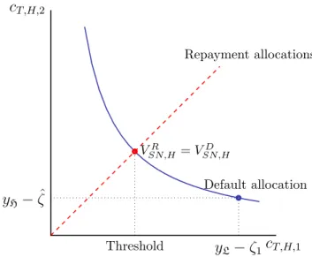
Proposition 4.1 (Default threshold of the subnational fiscal authority.) At the
highest level of debt for which a subnational fiscal authority prefers repayment to de-fault, T-good consumption under repayment equals the geometric average of initial- and terminal-period consumption of good T under default. The default threshold for the sub-national fiscal authority¯bSN is given by:
¯bSN = (1 +βω) (yL−ζ1) 1 1+βω yH−ζˆ 1+βωβω −(yL+βωyH). (39)
Proposition 4.1 implies that the debt default threshold for the subnational fiscal authority is increasing in the default costs in the two periods, in absolute value. We clarify both analytically and graphically how this threshold is determined.
For a generic subnational authority in a generic country in H, the value associated with default defined in (24) can be expressed as a function of quantities and prices, after imposing the intra-temporal choice of the household across goods T and N, as follows:21
VSN,HD =ahlog (yL−ζ1) +βωlog yH−ζˆ +β(1−ω) log (yH) i + (1−a) [log (lH,1) +βElog (lH,2)]. (40)
The value associated with repayment defined in (21), after imposing the optimal choice for assets traded and the equilibrium interest rate on risky debt (38), is given by a function of endowments, initial assets and prices and quantities in the N-good sector:
VSN,HR =a (1 +βω) log yL+βωyH+bH,1 1 +βω +β(1−ω) log (yH) + (1−a) [log (lH,1) +βElog (lH,2)]. (41)
The subnational authority takes its default decision by comparing the two values of repayment and default above described. The threshold in (39) is the level of assets for which these values are equal to each other. The subnational authority understands that its default decision has no impact on the equilibrium amount of labor employed in the
N-good sector. Hence, the subnational authority ignores the contribution of good N to welfare when deciding whether to default or to repay, as it perceives this contribution to be identical across the two decisions.
We now turn to analyze the implications of the subnational authority’s default decision for households’ consumption profile.
Corollary 4.1.1 (Consumption dynamics under default and repayment.) When
a subnational fiscal authority of a country in H is indifferent between defaulting and re-paying debt in the initial period, household consumption of good T in the initial period would be higher upon default:
yL−ζ1 >
yL+βωyH+ ¯bSN
1 +βω . (42)
Conversely, in the terminal period, high-default cost state, T-good household consumption is higher conditional on initial-period repayment.
yH−ζ <ˆ
yL+βωyH+ ¯bSN
1 +βω . (43)
In the terminal-period, low-default cost state, T-good household consumption is given by the endowment independently of initial-period choices.
21For ease of exposition, we also impose symmetry across countries in H and across subnational
au-thorities, so thatcN,H,t=
wH,tlH,t
cT,H,2 cT,H,1 yL−ζ1 yH−ζˆ Default allocation Repayment allocations Threshold VR SN,H =VSN,HD
Figure 2: Default threshold for the subnational fiscal authority. The two axes represent con-sumption ofT-good in the initial period and in the terminal period, in the high-default cost state. The blue, downward-sloping line is an indifference curve, representing the set of allocations that yield the same welfare as the default allocation to the representative household in H. From the point of view of the subnational fiscal authority, the contribution of good N to welfare is identical across all these allocations. The red, dashed, 45-degree, upward sloping line represents the set of allocations that are consistent with debt repayment and intertemporal optimality— i.e. with constant consumption of good
T, across periods. Each point of the line corresponds to a level of initial assets, bH,1, the higher the
further out from the origin. The intersection of the two curves determines the repayment allocation that yields the same welfare as default. The default threshold ¯bSN is the level of debt to which this allocation
corresponds. For higher levels of debt— i.e. closer to the origin than the intersection, default is preferred to repayment, and vice-versa for higher levels of debt.
Corollary 4.1.1 states that when the subnational fiscal authority defaults in the initial period, it causes its households’ current consumption to be higher than it would be upon repayment. Given the default threshold (39), this result follows from the assumption in (23). The household consumption profile crucially determines the impact of nominal rigidities on default, when decision-makers take them into consideration. We study this important force in the following subsections.
Figure 2 introduces a graphical framework through which to analyze the optimal de-fault decision, which will aid our analysis throughout the rest of this section. The figure displays the set of allocations that yield the same welfare as default, as well as those that are consistent with repayment, depending on initial-period assets. The default threshold is graphically determined as the intersection between these two sets of allocations— i.e. as the allocation where the subnational fiscal authority is indifferent between repayment and default. The location of the intersection can be use to gauge the relative attractiveness of default. The further is the intersection from the origin, the lower is the level of debt for which default is optimal.
4.1.2 Default by National Fiscal Authorities
When national fiscal authorities decide to repay or to default on external debt, they understand how their decision impacts on the severity of nominal rigidities in their country. National fiscal authorities internalize how the level of aggregate demand in the country depends on the default decision, and this consideration affects their relative incentive to default or repay. This is not the case for subnational authorities, who cannot affect demand at the national level. First, we discuss here the aggregate implications of the nominal rigidity that firms face, and how these affect the incentives of the fiscal authority. Second, we discuss the default decision of the national fiscal authority as a function of the severity of nominal rigidities.
Nominal Rigidities. Firms producing good N face downward wage rigidities. The
implication of these nominal rigidities is that the production of good N in each country may be bounded from above by domestic demand for the good itself. When nominal rigidities bind, firms only hire the amount of labor that is necessary to satisfy domestic demand for good N, given prices and wages that the rigidities imply. In equilibrium, if the nominal rigidity binds in H in the initial period, the price of good N and the wage are given by:
pN,H,1 =wH,1 =κ, (44)
and the amount of labor demanded by firms is given by
lH,1 = min 1−a a pT ,1cT ,H,1 κ , l . (45)
Nominal rigidities cause slackness in the economy, as firms only employ a fraction of the amount of labor that households supply inelastically. As a consequence, the amount of goodN that is produced and consumed in equilibrium is lower than the one that would be technologically feasible:
cN,H,1 =lH,1 ≤l. (46)
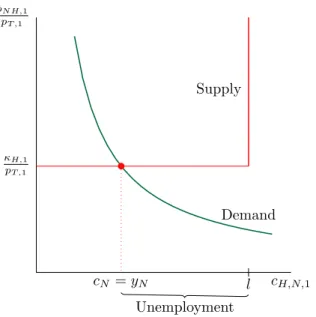
We graphically represent the equilibrium in the market for good N in Figure 3. The equilibrium allocation in this market lies at the intersection of the demand and supply for good N. Demand is the outcome of domestic households’ intra-temporal optimization, (6). Supply is given by an inverse L-shaped line. The horizontal segment of supply is given by the price that nominal rigidites imply when they bind. The vertical segment is in correspondence of the level of output that firms could produce if they employed the entire endowment of labor supplied by households.
The national fiscal authority understands that the default decision has effects on house-holds consumption of good T and, in turn, on demand for good N. Hence, the national fiscal authority has an incentive to alleviate the slackness present in the economy by in-creasing initial-period consumption of goodT, thereby expanding demand and output of good N.
pN H,1 pT ,1 cH,N,1 Demand l Supply κH,1 pT ,1 cN =yN Unemployment
Figure 3: Equilibrium in the market for goodN. The two axes represent consumption ofN-good and the its price relative to goodT, in the initial period, in a country inH. The green downward sloping curve represents demand for good N, (6). The red, inverse L-shaped line represents the supply of good
N, the combination of (2) and (35). The supply is vertical in correspondence of output produced when the entire endowment of labor is employed, and horizontal in correspondence of the price implied by downward wage rigidities. The intersection of demand and supply determines the equilibrium amount of goodN that is produced, and its relative price. The difference between the amount of labor supplied by households,l, and labor employed given output produced,yN stands for involuntary unemployment.
Values of Default and Repayment. The values associated with default and
repay-ment by the national fiscal authorities are analogous to the ones for subnational authorities (40) and (41), with the key difference that the former explicitly take into consideration domestic demand for good N. These values can be expressed as the sum of two terms. The first term equals the value to the subnational authority when nominal rigidities do not bind. The second term accounts for the severity of nominal rigidities.22
Formally, the value of default for the national fiscal authority can be written as:
VN F,HD = ( VD SN,H,F E if pT ,1 ≥p˜T ,D VD SN,H,F E+ (1−a) log p T ,1 ˜ pT ,D otherwise, (47)
where ˜pT ,D ≡κ1−aayL−lζ1 is the minimum initial-period price of good T that ensures that
nominal rigidities do not bind in a defaulting country inH. VSN,H,F ED denotes the value to the subnational fiscal authority under default and full employment—i.e. whencN,H,1 =l.
When nominal rigidities do not bind— i.e. when the price of good T is sufficiently high, the value for the national fiscal authority is identical to the full-employment one defined for the subnational authority. When the price of good T is sufficiently low, however, consumption of good N is low as well, and the national fiscal authority takes this fact into account when evaluating the effects of default on household welfare.
The value under repayment for the national fiscal authority can be expressed in an analogous way: VN F,HR = VR SN,H,F E if pT,1 ≥p˜∗T ,R(bH,1) VR SN,H,F E+ (1−a) log pT ,1 ˜ pT ,R(bH,1) otherwise, (48) where now ˜pT,R(bH,1) ≡ 1κ a−ay l(1+βω)
L+βωyH+bH,1 is defined similarly to ˜pT ,D and it represents the the minimum initial-period price of good T that ensures that nominal rigidities do not bind in a country in H that repays debt |bH,1|. VSN,H,F ER denotes the value to the
subnational fiscal authority under repayment and full employment. Again, the national fiscal authority understands that its choice to repay would imply a certain level of good-T
consumption and therefore a certain level of good-N output and consumption, given the effects of domestic demand on production in the presence of nominal rigidities.
Default Threshold. The severity of nominal rigidities crucially determines the level of
debt for which it is optimal for the national fiscal authority to default. We will consider the three relevant cases, depending on whether nominal rigidities never bind, they bind only upon repayment, or upon both default and repayment.
First, suppose that nominal rigidities do not bind, neither if the national fiscal au-thority repays debt, nor if it defaults. This is the case when
pT,1 ≥max{p˜T ,D,p˜T ,R(¯bN F,F E)} (49)
where ¯bN F,F E denotes the optimal default threshold, yet to be defined, for the national
fiscal authority when nominal rigidities never bind, neither under default nor under re-payment. In this circumstance, from comparing VD
N F,H and VN F,HR , the optimal default
threshold for the national fiscal authority is the same as the one for the subnational fis-cal authority, as domestic demand for good N plays no role in determining the optimal default decision:
¯
bN F,F E = ¯bSN. (50)
The national and subnational fiscal authority both correctly understand that, in this instance, the level of consumption of good N does not depend on whether they default or repay. At this default threshold, following Corollary 4.1.1, consumption of good T is higher upon default than upon repayment. Hence, the inequality in (49) can be expressed as pT ,1 ≥p˜T ,R(¯bN F,F E).
Second, consider the case where nominal rigidities always bind, both upon default and upon repayment— i.e. when
pT,1 <min{p˜T ,D,p˜T ,R ¯bN F,N R
}. (51)
The optimal default threshold in this setting is given by ¯bN F,N R. Again, it follows from
can be expressed in a very similar form to (39): ¯b N F,N R = (1 +βω) (yL−ζ1) yH−ζˆ βω p˜T ,R ¯bN F,N R ˜ pT ,D !1−aa 1 1+βω −(yL+βωyH). (52) The key difference between the two default thresholds (39) and (52) lies in the term that depends on the ratio of T-good prices that ensure full employment. This term captures the relative severity of nominal rigidities upon repayment and default, respectively. At the threshold, this ratio is greater than unity, since nominal rigidities are more detrimental to output upon repayment than upon default.23 Hence, this threshold is higher than the
one for the subnational fiscal authority, ¯bSN and default occurs for a lower level of debt (a
higher level of assets) than when nominal rigidities are not taken into account. Finally, condition (53) can be expressed as pT ,1 <p˜T ,D.
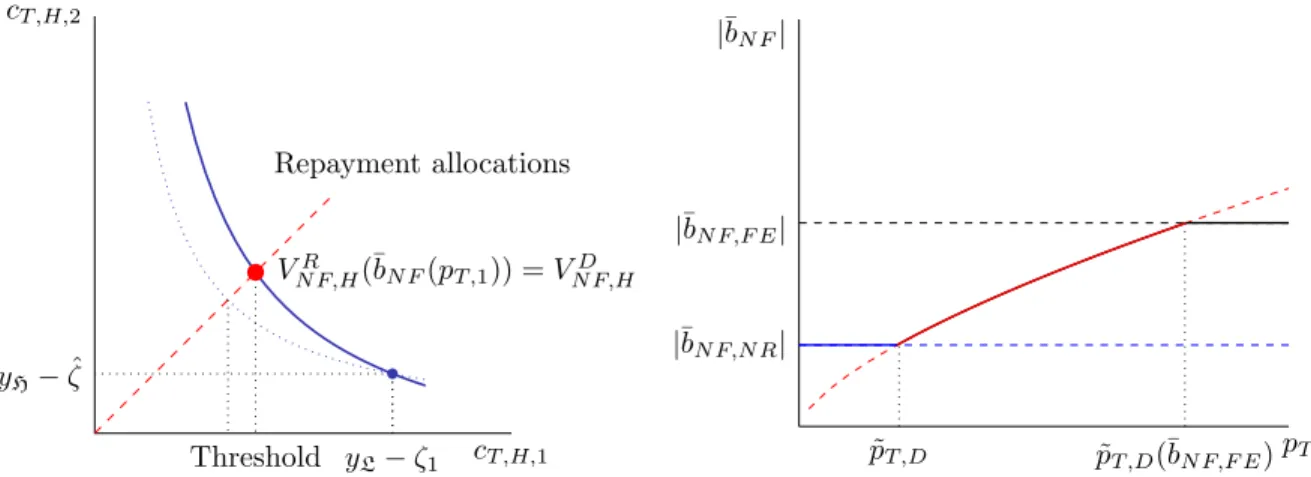
The left-hand side panel of Figure 4 graphically illustrates the impact of nominal rigidities on the default threshold for the national fiscal authority. The presence of nominal rigidities in the initial period increases the benefits of frontloading consumption in H. Graphically, this mechanism implies a north-eastward shift in the indifference curve that summarizes the allocations that yield the same welfare as default. Hence, the intersection with the set of allocations compatible with repayment lies to the right of the intersection in the absence of nominal rigidities. Thus, the level of debt for which default is optimal is lower when the national fiscal authority internalizes the effects of default and repayment on the level of domestic demand.
Finally, consider the case where nominal rigidities bind upon repayment but not under default. This is the case when
pT,1 ∈ ˜ pT ,D,p˜T,R ¯bN F,F E . (53)
In this setting, monetary policy crucially affects the default decision, as the economy would be at full employment conditional on default, but not upon repayment. By comparing the two value functions, (47) and (48), the default threshold is given by:24
¯b N F,F E−D = (1 +βω) (yL−ζ1) yH−ζˆ βω p˜T ,R ¯bN F,F E−D pT ,1 !1−aa 1 1+βω −(yL+βωyH). (54) Here, the term in the ratio of the prices ˜pT ,R andpT,1 implies that the default threshold is
increasing in the distance from full employment of the allocation under repayment. The more severe is unemployment upon repayment, the higher is that term and, therefore, the lower is the level of debt for which the national fiscal authority prefers to default.
We can now define the default threshold of the national fiscal authority as a function
23This follows from the result in Corollary 4.1.1. Appendix B.3.1 provides additional details, as well
as an explicit solution for the threshold.
24Again, Appendix B.3.1 provides additional details and an explicit expression for the threshold
¯b
cT ,H,2 cT ,H,1 yL−ζ1 yH−ζˆ Repayment allocations Threshold VR N F,H(¯bN F(pT ,1)) =VN F,HD |¯bN F,F E| |¯bN F,N R| |¯bN F| pT ˜ pT ,D(¯bN F,F E) ˜ pT ,D
Figure 4: Optimal default threshold under nominal rigidities. The left-hand side panel describes how nominal rigidities affect the default threshold of the national fiscal authority. In the presence of nominal rigidities, the benefit of frontloading consumption is higher. Hence, in comparison to Figure 2, the indifference curve shifts north-east. For the national fiscal authrority it is thus optimal to default at a lower level of debt, as the intersection with the set of repayment allocation implies a higher level of initial-period consumption. The right-hand side panel displays graphically the default threshold (55) of the national fiscal authority. The threshold is increasing in absolute value in the initial-period price of goodT: a higher price implies that nominal rigidities are less severe, and therefore default emerges for a higher level of debt (a lower level of assets).
of the price of good T in the initial period.
Proposition 4.2 The default threshold of the national fiscal authority as a function of
the price of good T is determined as the combination of the three thresholds that depend on the relative severity of nominal rigidities upon default and repayment:
¯bN F (pT ,1) = ¯ bN F,N R if pT ,1 <p˜T ,D ¯ bN F,F E−D(pT ,1) if pT ,1 ∈ ˜ pT ,D,p˜T ,R ¯bN F,F E ¯ bN F,F E if pT ,1 ≥p˜T ,R ¯bN F,F E (55)
The right-hand side panel of Figure 4 presents graphically the default thresholds described above.
Having characterized its default threshold, we can show that the additional benefit of default given by the relaxation of nominal rigidities makes it optimal for the national fiscal authority to default at lower levels of debt than for the subnational authority.
Corollary 4.2.1 (Default threshold of national fiscal authority.) The national
fis-cal authority finds it optimal to default for a lower level of debt than the subnational fisfis-cal authority: ¯bN F (pT ,1) ≤ ¯bSN . (56)
The result follows from comparing ¯bSN with ¯bN F (pT ,1). Appendix B.3.1 provides explicit
expressions for the thresholds.
Finally, if national fiscal authorities in all countries take the default-repayment decision in the initial period, an issue of absence or multiplicity of equilibria arises. This issue is
due to the binary and non-convex nature of the default decision, and to the two-way interaction between default and monetary policy. We discuss this issue in greater detail in Appendix B.3.2.
4.1.3 Default by a Coalition of National Fiscal Authorities
The national fiscal authorities of all countries in H can form a coalition and take jointly their default or debt repayment decision. The coalesced countries are aware that their decisions affect aggregate variables in equilibrium. In particular, the coalition under-stands that its decisions determine the conduct of policy by the supranational monetary authority, in pursue of its price-stability objectives. This result occurs due to the effects of default by all countries in H on the level and the distribution of consumption within the monetary union.
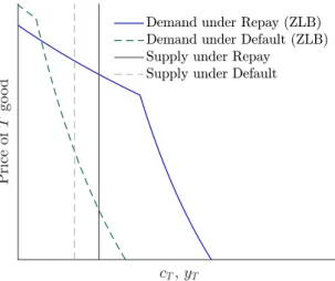
Countries in H may benefit from the ability to influence monetary policy, given the presence of nominal rigidities. The ability to engineer higher prices through default and, thus, to relax the severity of unemployment, reduces the relative benefit of debt repay-ment. First, we discuss in detail the equilibrium implications on nominal variables of default and repayment by the coalition of countries in H. Second, we present the val-ues of repayment and default for a representative household in H when the coalition of national fiscal authorities takes jointly the default or repayment decision. Third, we com-pare the optimal debt repayment threshold that emerges from this problem with the ones previously obtained for the individual national and subnational fiscal authorities. The absence of a limit on expansionary monetary policy plays a crucial role in this analysis. We analyze the presence of the zero lower bound in the next subsection, and we focus here instead on the setting where the action of the monetary authority is not constrained by this limit.
Aggregate Effects of Default and Repayment. A key force makes the default
de-cision by a coalition of countries in H different from that of an individual national fiscal authority. Crucially, the coalition considers how its decisions influence the equilibrium determination of nominal variables in the monetary union.
The main nominal variable of interest is the equilibrium price of good T in the initial period,pT ,1. A higher price of goodT implies that households reallocate demand towards
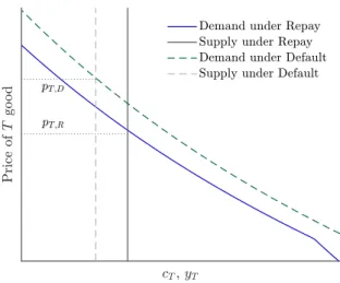
goodN, in turn reducing the severity of unemployment in countries in H, where nominal rigidities bind. In equilibrium, this price is determined by the intersection of the aggregate supply and demand for this good. Figure 5 provides a graphical representation of the equilibrium in this market.25
25For the purpose of Figure 5 and 6 below, we seta= 0.25, in line with the literature. The discount
factorβ is 0.99. We assume thatyH= 0.6 andyL = 0.4, so that we normalize aggregate endowment to
unity. The parameter that governs the downward wage rigidities,κ, equals unity. The monetary authority targets zero inflation in every period and it gives equal weights to the countries in the monetary union, meaningp∗ =π∗ = 1 andψ = 0.5. The fiscal authorities in countries inH inherit debt equal to yL/4.
Default cost in the initial period isζ1= 0.03 while the highest default cost in the second period is ˆζ= 0.3.
Figure 5: Equilibrium in the market for good T in the initial period, under default and repayment, in the absence of the zero-lower bound. Supply is given by the aggregate amount of good-T endowment, net of default costs if countries in H do not repay debt. Demand is given by the combination of the equilibrium conditions described in Section 3.6, with the exception of good-T market clearing. In particular, households’ intratemporal consumption allocation, the price stability objective of the monetary authority, and the output of goodN play a key role in determining demnad for goodT.
First, the aggregate supply of good T is given by the aggregate endowment of this good in all countries of the monetary union, net of default costs if relevant.
Second, the aggregate demand for good T is the combination of all equilibrium con-ditions described in Section 3.6, except for the T-good market clearing condition (32). Three main forces determine the level of aggregate demand for good T: households’ in-tratemporal demand for goods, the objective of the monetary authority, and the aggregate supply of goodN. The combination of the three gives rise to a downward sloping schedule in the cT-pT space. For a given price of good N intratemporal optimality implies that
households’ desired T-good consumption is decreasing in the price pT. In addition, for
the objective of the monetary authority to be satisfied, a high price of good T must be associated with a low price of good N. Hence, when the absolute price of goodT is high, its relative price is high, as well, implying a low desired consumption of good T, and contributing to the downward slope of the aggregate demand schedule.
Default and repayment by countries inH shift the intercept of the aggregate demand. When countries in H default, they consume in the initial period a higher amount of good T, for any given price. In addition, the aggregate supply of good T contracts, as resources are lost to the default cost ζ1. Hence, the upward shift of aggregate demand,
in conjunction with the lower aggregate supply of this good upon default, imply that the initial-period equilibrium price of good T is higher when the countries in H default on debt.
Values of Default and Repayment. The values associated by the coalition with
default and repayment resemble the ones of the subnational fiscal authority (40) and (41), with two key differences. First, the members of the coalition consider the spillover effect of T-good consumption on domestic demand for good N, exactly as the individual national fiscal authorities do. Second, the coalition internalizes the effect of its action
on aggregate equilibrium prices in the monetary union. Thus, when nominal rigidities bind for countries inH, the coalition understands how it would benefit from inducing an expansionary monetary policy. This is the crucial difference between the values of default and repayment for the individual national fiscal authorities and for the coalition of all countries in H.
Formally, the value of default for the coalition of national fiscal authorities can be expressed as follows:26 VD d N F ,H = ( VD SN,H,F E if p ∗ 1 ≥p∗1,D VD SN,H,F E + 1−a a+ψ(1−a)log p∗ 1 p∗1,D otherwise, (57) where p∗1,D ≡κ l1−aaa(yH)ψ(1 −a) (yL−ζ1) −(a+ψ(1−a))
is a threshold for the initial-period, price-level target of the monetary authority above which nominal rigidities would not bind in countries in H, conditional on their default. As previously, VSN,H,F ED denotes the value to the subnational fiscal authority under default and full employment—i.e. when
cN,H,1 = l. If the price-level target of the monetary authority is high enough, nominal
rigidities do not bind in H and the value of default for the coalition is the same as for the subnational fiscal authorities. If, instead, the price target is low enough, countries in
H face nominal rigidities and, due to low demand, firms in H produce a low amount of good N. In this instance, the coalition internalizes how households would benefit from the higher aggregate prices and less severe nominal rigidities that default implies.
Similarly, the value of repayment for the coalition depends on the initial-period price target for the monetary authority, as follows:
VR d N F ,H(bH,1) = VSN,H,F ER if p∗1 ≥p∗1,R(bH,1) VSN,H,F ER + a+ψ(11−a−a)log p∗ 1 p∗ 1,R(bH,1) otherwise, (58) where p∗1,R(bH,1) ≡ κ l(1 +βω)1−aa a (yH+βωyL−bH,1) ψ(1−a) (yL+βωyH+bH,1)
a+ψ(1−a) is again a threshold for the initial-period, price-level target of the monetary authority. For a price-level target above the threshold, nominal rigidities would not bind in H upon repayment. The threshold is decreasing in the level of initial-period in assets in H. When debt is lower (assets are higher), repayment of debt is consistent with a relatively high level of demand in H, hence a relatively low target of the monetary authority is sufficient to ensure full employ-ment. VR
SN,H,F E is the previously defined value for the subnational fiscal authority under
repayment and full employment. The coalition of national fiscal authorities understand that its actions have effects on aggregate prices in the monetary union, as it does under default. In particular, the coalition understands that the severity of nominal rigidities in
H depends on the level of initial assets bH,1, given the implications of this quantity on
the level of domestic aggregate demand, as well as on the equilibrium price pT ,1 that is
determined in the monetary union.
The consideration of the equilibrium determination affects the threshold on initial