Full Terms & Conditions of access and use can be found at
https://www.tandfonline.com/action/journalInformation?journalCode=tejr20
ISSN: (Print) 2279-7254 (Online) Journal homepage: https://www.tandfonline.com/loi/tejr20
Geo-spatial text-mining from Twitter – a feature
space analysis with a view toward building
classification in urban regions
Matthias Häberle, Martin Werner & Xiao Xiang Zhu
To cite this article: Matthias Häberle, Martin Werner & Xiao Xiang Zhu (2019): Geo-spatial text-mining from Twitter – a feature space analysis with a view toward building classification in urban regions, European Journal of Remote Sensing, DOI: 10.1080/22797254.2019.1586451
To link to this article: https://doi.org/10.1080/22797254.2019.1586451
© 2019 The Author(s). Published by Informa UK Limited, trading as Taylor & Francis Group.
Published online: 13 Mar 2019.
Submit your article to this journal
Article views: 2
Geo-spatial text-mining from Twitter
–
a feature space analysis with a view toward
building classification in urban regions
Matthias Häberle a, Martin Wernerband Xiao Xiang Zhua,b
aSignal Processing in Earth Observation (SiPEO), Technical University Munich (TUM), Munich, Germany;bRemote Sensing Technology Institute, German Aerospace Center (DLR), Weßling, Germany
ABSTRACT
By the year 2050, it is expected that about 68% of global population will live in cities. To understand the emerging changes in urban structures, new data sources like social media must be taken into account. In this work, we conduct a feature space analysis of geo-tagged Twitter text messages from the Los Angeles area and a geo-spatial text mining approach to classify buildings types into commercial and residential. To create the feature space, broadly accepted word embedding models like word2vec, fastText and GloVe as well as more traditional models based on TF-IDF have been considered. A visual analysis of the word embeddings shows that the two examined classes yield several word clusters. However, the classification results produced by Naïve Bayes support vector machines, and a convolutional neural network indicates that building classification from pure social media text is quite challenging. Furthermore, this work illustrates a base toward fusing text features and remote sensing images to classify urban building types.
ARTICLE HISTORY
Received 13 July 2018 Revised 18 February 2019 Accepted 21 February 2019
KEYWORDS
Geo spatial text mining; feature space analysis; word embeddings; social media; urban structures
Introduction
A significant phenomenon in the twenty-first century is the migration from small- or middle-sized urban com-munities into mega cities. By the year 2050, around 68% of people will live in metropolises (Taubenböck & Wurm, 2015; United Nations, 2018). These develop-ments lead to fundamental changes in urban city struc-tures. In order to observe and to understand these dynamic changes of settlement patterns, city structures or the temporal development of building areas are going to need the adoption of new and dynamic sources of information augmenting visual and morphological infor-mation available from remote sensing. In this context, social media data promise to provide useful insights into the human aspects of urban dynamics that do not neces-sarily manifest in morphology. In addition, social media provides a very timely source of information given that users feed social media platforms with a sheer number of different kinds of information every second.
Three types of information provided by geo-refer-enced social media can be distinguished: the occur-rence of a posting in space, the metadata about the user including number of friends, likes, number of message citations, keywords (often given inline in the form of hashtags) and the message content itself.
We expect that all three types of information con-tain hints on intra-urban characteristics in general, but not for each and every message. In this paper, we want to concentrate on social media text for
geo-located tweets. Though we are restricting attention to geo-located text messages, it should be noted that language itself can provide geographic references through spatial language (next to, near, etc.) as well as landmarks (e.g. restaurant name, touristic attrac-tions, etc.).
In this work, we focus on the social network Twitter (tweets). Twitter is a microblogging service with 336 million daily active users across the world (Twitter,2018b). Users generate short (length is actu-ally constrained) text messages which could be enriched with images, videos, keywords and the men-tion of a friend’s twitter account or of a certain land-mark. The official Twitter API provides free access for streaming a subset of tweets and simultaneously deli-vers detailed metadata about the tweet, the user and the place. Particularly interesting for our work is the raw tweet string combined with precise geolocation.
Contribution
In this work, we investigate the feasibility to classify Los Angeles building instance type (commercial/resi-dential) from Twitter text messages (tweets) without integrating further metadata. This task is challenging due to poor text quality, limited text length (up to 280 characters) of the messages and the lack of a suffi-cient amount of precisely geo-located tweets. To tackle those hurdles, we investigate the feature space of the two classes produced by geo-tagged Los
CONTACTMatthias Häberle [email protected] Signal Processing in Earth Observation (SiPEO), Technical University Munich (TUM), Arcisstraße. 21, Munich 80333, Germany
EUROPEAN JOURNAL OF REMOTE SENSING https://doi.org/10.1080/22797254.2019.1586451
© 2019 The Author(s). Published by Informa UK Limited, trading as Taylor & Francis Group.
This is an Open Access article distributed under the terms of the Creative Commons Attribution License (http://creativecommons.org/licenses/by/4.0/), which permits unrestricted use, distribution, and reproduction in any medium, provided the original work is properly cited.
Angeles Twitter text messages with three different broadly accepted word vector model implementations namely word2vec, fastText and GloVe. We visualize and analyze the internal structure of these feature spaces. For classification experiments, we utilize pre-trained word vectors provided by the respective authors in order to avoid under- as well as over-fitting in the embedding step. To classify the word embeddings, we used a convolutional neural network (CNN). Support vector machines (SVM) as well as Multinomial Naïve Bayes classifiers have been applied to sparse representations of text based on TF-IDF. The received features could be used for fusion with remote sensing data to improve building type or land use classification.
Related work
Social media data offers a broad field of applications, for instance, sentiment analysis and demographic charac-teristics (Mitchell, Frank, Decker Harris, Sheridan Dodds, & Danforth,2013), emotion detection and sar-casm prediction (Felbo, Mislove, Søgaard, Rahwan, & Lehmann, 2017) or competitor analysis in the pizza industry (He, Zha, & Li, 2013). The usage of social media data turned out as valuable source for geospatial research. For example, changes in Flickr images, night lights and news could be employed to detect conflicts or refugee movements (Levin, Ali, & Crandall,2018). Geo-located Twitter data are used in Sobolevsky et al. (2018) to show that Twitter users with a social relationship share similar mobility patterns.
The combination of additional data sources and remote sensing has been showed in various studies. For example, the usage of OpenStreetMap data und Landsat images indicate improved land use classification results for 24 classes (Hu, Yang, Li, & Gong,2016). Therefore, the fusion of remote sensing and social media data seems to be an innovative way of augmenting remote sensors. One of the applications of social media and remote sensing is weather-caused disasters like floods. For exam-ple, the combination of remote sensing data and Twitter messages results in improvement of flood detection and predicting (Wang, Skau, Krim, & Cervone,2018), and flood risk management (de Assis, Herfort, Steiger, Horita, & Porto de Albuquerque, 2015). The general applicability of social media text messages to the building instance classification task has been shown previously using techniques such as LDA (Blei, Ng, & Jordan,
2003) and LSTM recurrent neural networks on georefer-enced tweets from Munich (Huang, Taubenböck, Mou, & Zhu, 2018). Twitter data can also be exploited to understand whether informal settlements have a differ-ent social media activity pattern as opposed to formal settlements in Mumbai (Klotz, Wurm, Zhu, & Taubenböck, 2017). The urban structural types have been detected by high-resolution earth observation
methods (HR Quickbird data). The study revealed that in informal settlements, the Twitter activity (in propor-tion to the populapropor-tion density) was not as demanding as in formal settlements. By means of this digital coldspots of the informal areas, it was possible to discriminate the two settlement types to a certain extent. Hence, the usage of Twitter and remote sensing data contributed to the understanding of socio-spatial characteristics of the megacity Mumbai.
Methods
In this section, we introduce the methodology used for the feature space analysis and the building classification task. We first explain two employed text representation methods allowing for represent-ing text as a constant-size vector in order to learn from these fixed-size representations. Among these, we explain the classical word count sparse matrix representation normalized using TF-IDF as well as text embeddings based on skip-gram and continu-ous-bag-of-words (CBOW) models.
Text representation for machine learning
Given the fact that many machine learning algo-rithms expect that instances have a constant size (e. g. a number of features), methodology is needed to transform variable-length text into a feature space representation with constant dimension.
The most traditional approach is to count word occurrences in the text. Therefore, a vocabulary is fixed, and for each text, a vector is being generated containing the frequency of every word of the vocabu-lary in the document. In this context, however, selecting a good vocabulary is extremely difficult: some frequent words are completely meaningless (called “stop words”), some frequent words are meaningless to the given task or corpus of text (called“corpus-specific stop words”), and for rare words, it is difficult for a machine learning algorithm to collect enough evidence of the meaning of the word for a given task. Therefore, a traditional approach is to remove a fraction of frequent and infrequent words from the vocabulary.
In addition to that, a measure of importance for each word in a document related to a corpus of text has been proposed and is widely known as TF-IDF (term frequency-inverse document frequency). The term frequency (TF) is the number how frequently a term tappears in a documentd.
tf t;ð dÞ ¼ ft;d
maxft0;d:t02d
The inverse document frequency (IDF) denotes the words importance (Spärck Jones, 1972). The IDF term is calculated as follows:
idf t;ð DÞ ¼ log N
1þjfd2D:t2dgj
In this equation,N is the number of documents in a corpus. The addition of 1 in the denominator pre-vents a division through zero iftis not ind. Finally, the TF-IDF score is calculated as follows:
tfidf t;ð d;DÞ ¼tf t;ð dÞidf t;ð DÞ
IDF has, for example, been applied to find interesting research articles on the Internet (Bollacker, Lawrence, & Giles,1998). The difference between TF and IDF is that TF treats every word as equally important. In contrast, IDF assigns less importance to words which come up very often in the corpus.
A count-based vocabulary construction, e.g. taking the vocabulary to be all words except the pf percent most frequent and the pr percent least frequent, is usually combined with TF-IDF for each occurrence of a word transforming a set of text messages into a sparse numeric feature matrixX¼xijin whichxijcontains the TF-IDF score of wordjin documenti. In this way, the machine learning problem can be formulated to learn a modelf trained on the rows of the matrixX.
Sparse text mining methods
When a text corpus is represented by means of the methods of the previous section, we obtain a sparse feature matrixX in which the columns are related to words and the rows are documents in the corpus. One way to treat this representation is through Naïve Bayes classification. In this setting, it is falsely assumed that all features are statistically independent. Under this assumption, classification can be per-formed using Bayes rule on each and every feature individually and combining the results through mul-tiplication (Hand & Yu, 2001). For the case of text mining, using a multinomial distribution for the indi-vidual features makes sense, because they do not model normally distributed measurements but occur-rences. Though only integer values are theoretically sound in this setting, experimentation has shown that it is practicable to use fractions such as TF-IDF, too. Another widely accepted family of classifiers for such sparse, high-dimensional data is given by SVMs. In SVMs, the model tries to maximize linear separa-tion between classes by applying non-linear transfor-mations (Cortes & Vapnik, 1995). SVMs can be formulated as optimization problems and we used a representation of SVMs for stochastic gradient decent which allows adding penalties for regularization. In combination with TF-IDF, Dadgar, Araghi, & Farahani (2016) used an SVM to classify news. Furthermore, Benkhelifa & Laallam (2016) applied SVMs and Naïve Bayes to Facebook post topic classification.
More sophisticated and naturally inspired (LeCun & Bengio, 1995) classifiers are CNNs (LeCun, 1989). The structure of a CNN consists of one orm convolu-tional layers which applyingn-dimensional kernel fil-ters to produce a feature map of the input data. For text and sequence analysis, one-dimensional filters combining neighboring feature values are widely used. For computer vision, two-dimensional filters combine small rectangles across the image into new values. Typically, each convolution layer is succeeded by a pooling layer which reduces the created feature map by taking a summary of neighboring pixels. Max pooling, for example, takes a nn window and extracts the maximum value within that window from sliding over the feature map. As this step is often applied without overlap, it can be used to reduce the dimensionality of the feature map and therefore decrease the number of output neurons. Then, fully connected or dense layers are often used to classify the resulting features extracted by the convolution and pooling layers using a final softmax layer. CNNs are well-known approaches in computer vision tasks (He, Zhang, Ren, & Sun, 2016; Simonyan & Zisserman,
2015; Zhang et al.,2018). However, they also proved themselves useful in the field of natural language pro-cessing. For text classification, a CNN was applied with a little bit of hyperparameter tuning and pre-trained word vectors (Yoon,2014). In election prediction tasks with Twitter text data, CNNs in combination with word vector models can outperform traditional mod-els like SVMs with TD-IDF (Yang, Macdonald, & Ounis, 2018). However, they also need more data to train. Badjatiya, Gupta, & Varma (2017) used CNNs among others to classify the sentiment of a tweet to detect hate speech in Twitter text messages.
Word embeddings
It has been recently discussed that sparse text repre-sentations using TF-IDF are limited by the size of the vocabulary needed to encode the significant part of a language. When the texts are from a narrow domain and there is a small vocabulary (say about 1000 words) that can cover the given application, then TF-IDF is very successful. When such a vocabulary does not exist or is very difficult to find, then it will practically be growing putting more difficulties from language encoding into the machine learning part (Bengio, Ducharme, Vincent, & Jauvin, 2003). In this setting, word embeddings have been proposed in which each word is represented as a unique multi-dimensional feature vector in a vector space of cho-sen dimension. The general idea is to place feature vectors for words that co-occur frequently in a joint context near in space. This co-occurrence is often defined by a window of neighboring words, though other definitions of context can be applied.
word2vec
Mikolov, Chen, & Corrado (2013) proposed two pre-diction-based log-linear approaches for creating mul-tidimensional word embeddings. The CBOW model is trying to predict a word in the middle ofncontext words to its left and right. On the other hand, The Continuous Skip-gram Model attempts to predict n
context words based on a word in the middle of the context words. The structure of the models is almost similar to the feedforward neural language model proposed by Bengio et al. (2003). But Mikolov et al. (2013) omit the computational intensive non-linear hidden layer to reduce training time for large text corpora. Word vectors computed by the skip-gram model show better performance on validation tasks, e.g. word analogy task,1yet demonstrate longer train-ing times.
fastText
Unlike word2vec and GloVe, fastText (Bojanowski, Grave, & Mikolov, 2017) takes subword information into account. They propose an extension of the con-tinuous skip-gram model to learn word representa-tions by character n-grams. For example, the word house is transferred to a charactern-gram of length
n = 3 as <ho, hou, ous, use, se>. The “<” at the beginning and the“>” at the end of a word are used as boundary symbols to flag the beginning and the end of a word. To learn the representation of each word, the word itself is added to the set of n-grams. Words are represented as the sum of their character
n-grams vectors. Because of the additional morpho-logical information due to character n-grams, fastText achieves better results as word2vec in syn-tactical word analogy task and in informal language, whereas in the semantic category, word2vec performs better (Bojanowski et al.,2017).
GloVe
Instead of using a shallow context window like skip-gram or CBOW, the count-based model GloVe (Pennington, Socher, & Manning,2014) utilizes the whole statistics of word co-occurrences in a given corpus and trains in an unsupervised manner. To identify if two wordsiandjare related, their co-occurrences probabilities with“probe” wordskare examined (Pennington et al.,2014). If, for example, two words are sharing the same context withk, e.g. appear in the same topic, the ratio of the co-occur-rence probabilities should be small. By contrast, if the words are not related with each other, the ratio of the probabilities is high. Using the same validation tasks like Mikolov et al. (2013), GloVe outperforms CBOW and skip-gram models, for example in the word analogy task, partially with smaller training corpora and vector sizes
(Pennington et al., 2014). With their findings, Pennington et al. controvert discussions (e.g. Baroni, Dinu, & Kruszewski,2014) about the superiority of pre-diction-based models like word2vec or fastText over count-bases models. They argue that both prediction-and count-based methods are not fundamentally differ-ent,“… but the efficiency with which the count-based methods capture global statistics can be advantageous”. (Pennington et al.,2014, p. 1541).
Dataset
In this section, we describe how we obtained the Los Angeles Twitter data, show relevant corpus statistics and explain how we conducted text pre-processing. Tweets
The tweets were obtained via the official Twitter API (Twitter, 2018a) from Los Angeles in a period of 6 months. For our research, we only used georefer-enced tweets. We executed simple pre-processing steps to remove all numbers, punctuations, special characters (e.g. @) and web URLs. In addition to that, all characters were set to lower case to avoid distinctions of identical words like “House and “house”. Furthermore, we excluded stop words (e.g.
the, are, is, etc.) and words which are smaller than three characters because of the highly irregular lin-guistic properties such as single characters.
Corpus statistics
Table 1 shows the corpus statistics which give a brief overview of the collected dataset and its shape after several pre-processing methods. Altogether, we streamed 599,385 geo-located tweets with about 10.5 million words from Los Angeles in a time period of 6 months. Before executing text pre-processing, tweets show a mean of 17.2 words per tweet. After removing all numbers, special characters and words with less than three characters, the mean length of a tweet dropped to 10.6 words. Stop-word removal additionally leads to a decrease of the mean length to 7.6 words per tweet.
Since one goal is to classify residential/commercial building types, we assign labels provided by the crowd-sourcing GIS OpenStreetMap (OSM).2 In specific, we conducted a spatial nearest neighbor join of Los Angeles OSM building polygons and georeferenced tweets. We removed all tweets that cannot be safely assigned to the direct vicinity of a building given by a Euclidean“ dis-tance” of 0.001 in the WGS84 coordinate space. This distance translates to a few meters in the area of Los Angeles. The OSM building polygons had to possess either the building label “commercial or “residential”. After the join, the residential class shows 161,996 and 1Kingis toqueenasmanis to ___?
the commercial class 437,389 tweets. Due to the fact of a clear disparity of the two classes, we decided to under-sample the both classes to 150,000 tweets per class (He & Garcia,2009). After this step, the mean length of a Tweet slightly changed from 7.6 to 7.7.
Top words
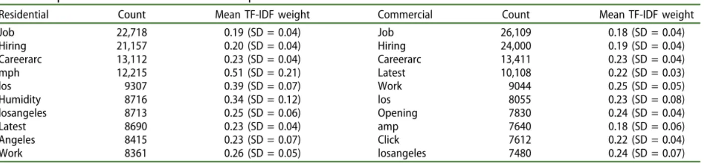
Also we were interested in the different top 10 words per class of the undersampled dataset to understand if they demonstrate commonalities or if they show completely different top words.Table 2shows the top 10 words for each class. It is noticeable that the top three words of both classes are the same. Note that the word count of these words with a rather commercial meaning is actually slightly higher for the commercial class. In addition to that, it is apparent, that the mean TF-IDF weights of the words are quite low due to the fact, that these words are appearing in high frequency in the dataset. In other words, they cannot contribute much information to the given classification task.
Train and validation split
Instead of randomly splitting the dataset into a train and validation set, we conducted a spatial split in train and validation sets. Therefore, we split the tweets in four spatial parts by means of their coordinates. First, the data are split on the horizontal axis using the median of
the longitude coordinates. Then, each split is further divided using the median of the latitude within this split.Figure 1depicts the results of the spatial split. We train the classifiers on three parts and estimate perfor-mance using the fourth part of the data for validation. This approach guarantees that the validation data are from another area of Los Angeles and, therefore, spatial overfitting is avoided. This results in a dataset containing 224,594 tweets for training as well as 75,406 tweets for validation.
Feature space analysis
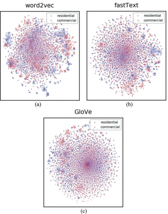
For the feature space examination, we created word embeddings for each class by means of the three intro-duced word embedding models. The parameters are cho-sen as proposed by the authors of the models except for the embedding dimensionality which we set tod= 300 and word window size set to 5 words. To visualize the created embeddings, we usedt-SNE (van der Maaten & Hinton,2008) to reduce the dimensionality of the most frequent 3000 word vectors down to 2 dimensions.
Figure 2shows thet-SNE plot of the most frequent words for word2vec, fastText and GloVe. The word2vec embedding shows a kind of uniform distribution of strong clusters of both classes without a clear central area for the majority class. For fastText, the center of the image shows a commercial cluster and the right outer
Table 1.Corpus word statistics.PP= pre-processing;sw= stop words;w < 3= words smaller than three characters;“+”= includes, “−”= excludes; smaller than three characters.
Dataset Statistics Residential Commercial Total
Full dataset
Raw tweets 161,996 437,389 599,385
Raw words 2,725,827 7,709,649 10,435,476
Unique words before PP 200,578 495,676 636,450
Unique words after PP (+ sw,–w < 3) 199,832 494,816 635,568 Unique words after PP (−sw,–w < 3) 83,471 178,666 220,187
Mean words/tweet before pp 16.8 17.6 17.2
Mean words/tweet after PP (+ sw,–w < 3) 10.4 10.9 10.6 Mean words/tweet after PP (−sw,–w < 3) 7.6 7.7 7.6
Undersampled dataset
Raw tweets 150,000 150,000 300,000
Raw words 2,519,323 2,640,587 5,159,910
Unique words before PP 200,400 248,948 449,348
Unique words after PP (+ sw,–w < 3) 83,533 101,892 185,425 Unique words after PP (−sw,–w < 3) 83,415 101,777 185,192
Mean words/tweet before PP 16.8 17.6 17.2
Mean words/tweet after PP (+ sw,–w < 3) 9.2 9.7 9.5 Mean words/tweet after PP (−sw,–w < 3) 7.6 7.8 7.7
Table 2.Top 10 class words of the undersampled dataset with word counts and mean TF-IDF scores with standard deviation.
Residential Count Mean TF-IDF weight Commercial Count Mean TF-IDF weight Job 22,718 0.19 (SD = 0.04) Job 26,109 0.18 (SD = 0.04) Hiring 21,157 0.20 (SD = 0.04) Hiring 24,000 0.19 (SD = 0.04) Careerarc 13,112 0.23 (SD = 0.04) Careerarc 13,411 0.23 (SD = 0.04) mph 12,215 0.51 (SD = 0.21) Latest 10,108 0.22 (SD = 0.03) los 9307 0.39 (SD = 0.07) Work 9044 0.25 (SD = 0.05) Humidity 8716 0.34 (SD = 0.12) los 8055 0.23 (SD = 0.08) losangeles 8713 0.25 (SD = 0.06) Opening 7830 0.24 (SD = 0.04) Latest 8690 0.23 (SD = 0.04) amp 7640 0.18 (SD = 0.06) Angeles 8415 0.23 (SD = 0.07) Click 7612 0.22 (SD = 0.04) Work 8361 0.26 (SD = 0.05) losangeles 7480 0.24 (SD = 0.07)
areas a residential word cluster. Finally, for the GloVe embedding, a concentrated commercial cluster is visible in the image center and a few smaller residential and commercial word clusters can be seen to the left outside area. In summary, however, there seems to be no clear separation of the two classes in any of the embeddings highlighting the hardness of the task and the fuzziness of the association of text content to building functions. Still, clustered areas like the blue area on the top-left corner of the word2vec embedding support the expec-tation that some tweets contain significant and suffi-cient information for this classification task.
Experiment
In this section, we present our experimental setup. First, we briefly introduce the pre-trained word vec-tors obtained from word2vec, fastText and GloVe. Furthermore, we describe the utilized classifiers and the used architectures as well as their hyperparameter settings. Finally, we discuss the validation method for the building classification task.
Pre-trained word vectors
The pre-trained word vectors are obtained from the project websites of word2vec,3 fastText4and GloVe5
Consider Table 3 for word vector details. Each pre-trained word vector was pre-trained with different text corpora, e.g. Google News Dataset, and they therefore provide a wide range of vocabulary.
Support-vector machine and Naïve Bayes
For baseline classification, we used a SVM and a multinomial Naïve Bayes classifier each with TF-IDF for feature extraction. The SVM was constructed using stochastic gradient decent with hinge loss, l2 penalty and 5 epochs.
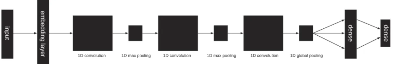
Convolutional neural network
In addition, we trained for CNNs with an input layer followed by a word embedding layer (seeFigure 3). The word embedding layer is initialized with the pre-trained word vectors obtained from word2vec, fastText and GloVe. The embedding layer is followed by three 1D convolutional layers with a filter size of 128 and a kernel size of 5. As activation function, we applied rectified linear units (ReLU). Each 1D convolutional layer is fol-lowed by a 1D max pooling layer with a pooling size of 5. The last convolutional layer is succeeded by a global max pooling layer. The convolutional and max pooling layers are followed by two fully connected layers to conduct
Figure 1.Spatial validation split of the undersampled dataset. The gray area represents the training set and the black area the validation set.
3https://code.google.com/archive/p/word2vec/
4https://fasttext.cc/docs/en/english-vectors.html 5https://nlp.stanford.edu/projects/glove/
classification. The last fully connected layer has two out-put units and its activation is handled by the softmax activation function. The network was trained for five training epochs. As optimizer, we used RMSprop and no dropout was applied.
Results
Table 4 illustrates the validation results of the three different models. The multinomial Naïve Bayes model shows in the residential class low recall values
which indicates that the classificator could not grasp the concept of the residential buildings. In contrast, the recall at the commercial class yields a higher value, which could be a sign of learning commercial class text attributes. If one considers the results of the SVM model, it is apparent that the recall number of the residential class is low compared to the Naïve Bayes result. On the other hand, the commercial-class recall value outperforms the results of the other models. The CNNs with the pre-trained word embedding layer perform slightly better on the
Figure 2.t-SNE plots of the embedded top 3000 residential and commercial class words. Table 3.Pre-trained word vector details.
Implementation Name Dimensions Words Text source word2vec GoogleNews-vectors-negative300 300 3 M Google News dataset, 100B words GloVe (CC) glove.42B.300d 300 1.9 M Common Crawl
GloVe (TW) glove.twitter.27B 200 1.2 M Twitter, 2B tweets
fastText wiki-news-300d-1M 300 1 M Wikipedia 2017, UMBC webbase corpus, statm.org news dataset
residential class as the SVM and Naïve Bayes. One exception is the CNN with the pre-trained GloVe (CC) embeddings which is topped by the Naïve Bayes. In the commercial class, the CNNs (except the CNN with word2vec) beat the Naïve Bayes, yet they are all outperformed by the SVM.
Discussion
It is quite evident that the commercial class yields higher recall values obtained by all used models, whereas the residential class shows better perfor-mance on the precision metric. Table 2 delivers a possible explanation. One possible assumption for the SVM and the Naïve Bayes performance could be that the TF-IDF weights of the listed top-class words are low. This means that the word frequency of each word and the expectation to see this word within all documents (tweets) are high and TF-IDF weighs them as low information entities. The flashy commer-cial-class recall value of the SVM could be the indica-tion of overfitting due to low informaindica-tion words.
If the top three words of each class are the same (“job”, “hiring” and “careerarc”) and further sharing other words like“work”(just in a different order), it is assum-able that the classifier guesses the class. In this case, it might guess the commercial class not only because of the same words but also of the higher word counts of the top three commercial class words. Other top words of both classes are “losangeles”, “los” and “angeles”. Where “losangeles” is spelled together, “los” and “angeles” is the outcome of tokenization of the text pre-processing steps. Since both classes show these phrases, the classi-fiers might have problems distinguishing both classes by
top words. However, if the word count at the commercial class is higher, the classifiers could assume that every given sample belongs to the commercial building class. As can be seen fromTable 1, both the complete and the undersampled datasets contain more unique words in the commercial class. This circumstance suggests that the language of commercial class tweets uses a richer voca-bulary and a wider range of phrases. In fact, this means that normalizing the classes with respect to the occur-rence of tweets might be misleading. Instead, advanced vocabulary constructions should be discussed taking care that both classes materialize with similar numbers of words.
Conclusion
In this work, we conducted a feature analysis for a building classification task based on Twitter text messages from the Los Angeles area. By the help of word embedding models, we generated word vectors of the top 3000 words of each class. The plots of the feature space show several word clusters per class and at the same time a huge overlap. Consequently, preliminary classification results indicated that the building classification task providing pure text fea-tures for the applied classification techniques is rather challenging. To the contrary, however, one can also conclude that some tweets contain signifi-cant information about the two classes depending on their actual location in the feature space: if they are part of a cluster, we expect that they can be directly classified – if they are not part of any cluster, we don’t expect a classifier to be able to assign them to one of the classes using this feature space alone. In
Figure 3.Convolutional neural network with embedding layer initialized with pre-trained word vectors obtained from word2vec, fastText and GloVe.
Table 4.Classification results.
Residential Commercial
Precision Recall F1 Precision Recall F1 Accuracy
Naïve Bayes 0.56 0.44 0.49 0.51 0.63 0.49 0.53 SVM 0.60 0.23 0.33 0.50 0.83 0.62 0.52 CNN fastText 0.59 0.45 0.51 0.53 0.66 0.59 0.54 GloVe (CC) 0.59 0.40 0.48 0.52 0.69 0.59 0.54 GloVe (TW) 0.58 0.47 0.52 0.52 0.64 0.57 0.54 word2vec 0.60 0.51 0.55 0.57 0.63 0.57 0.56
order to improve classification results, one could (i) collect more training examples to counteract the difficulties of unbalanced datasets, (ii) try to provide a broader variety of texts of the different classes and (iii) improve text pre-processing and embedding methods to account for class imbalances and word count imbalances. To tackle class overlap and imbal-ance, one could apply advanced classification meth-ods like abstaining (Balsubramani, 2016; Chow,
1957). To improve text pre-processing and embed-ding methods, one could exclude top-class overlap-ping words from classification as corpus-specific stop words to generate a more explicit feature spaces for each class.
Future work could comprise training on more than one city and the validation with other cities. In combination with the latter, multilingual word vec-tors could be used to cover multilanguage text mes-sages in one city or area. Topic analysis could be used to explore if different building types or areas indicate different topics and in order to reduce the dimen-sionality of the TF-IDF-based feature spaces.
Finally, this work provides a first step toward fusion of social media text features and remote sen-sing imagery. The combination of space born data and constantly updated social media texts could pro-vide extended and up-to-date information about intra-urban characteristics and even socioeconomic structures in a rapidly changing urban environment in the twenty-first century.
Disclosure statement
No potential conflict of interest was reported by the authors.
Funding
We gratefully acknowledge the support of the European Research Council (ERC) under the European Unions Horizon 2020 research and innovation programme (grant agreement No [ERC-2016-StG-714087], Acronym: So2Sat), Helmholtz Association under the framework of the Young Investigators Group “SiPEO” (VH-NG-1018, www.sipeo.
bgu.tum.de).
ORCID
Matthias Häberle http://orcid.org/0000-0001-9550-5252
References
Badjatiya, P., Gupta, S., & Varma, V. (2017).Deep learning for hate speech detection in Tweets. Proceedings of the 26th International Conference on World Wide Web Companion (pp. 759–760).
Balsubramani, A. (2016). Learning to abstain from binary prediction.ArXiv.Org, (1602.08151).
Baroni, M., Dinu, G., & Kruszewski, G. (2014).Don’t count, predict! A systematic comparison of context-counting vs. con-text-predicting semantic vectors. Proceedings of the 52nd Annual Meeting of the Association for Computational Linguistics (pp. 238–247). Baltimore, MD.
Bengio, Y., Ducharme, R., Vincent, P., & Jauvin, C. (2003). A neural probabilistic language model. Journal of Machine Learning Research,3, 1137–1155.
Benkhelifa, R., & Laallam, F.Z. (2016). Facebook posts text classification to improve information filtering. Proceedings of the 12th International Conference on Web Information Systems and Technologies (WEBIST 2016), Rome, Italy. Blei, D.M., Ng, A.Y., & Jordan, M.I. (2003). Latent
Dirichlet allocation. Journal of Machine Learning Research 3(4–5), 993–1022.
Bojanowski, P., Grave, E., & Mikolov, T. (2017). Enriching word vectors with subword information.Transactions of the Association for Computational Linguistic,5, 135–146.
doi:10.1162/tacl_a_00051
Bollacker, K.D., Lawrence, S., & Giles, C.L. (1998).CiteSeer: An autonomous Web agent for automatic retrieval and identification of interesting publications. AGENTS ’98 Proceedings of the second international conference on Autonomous agents (pp. 116–123). Minneapolis, MN. Chow, C.K. (1957). An optimum character recognition
system using decision functions. IRE Transactions on Electronic Computers, EC-6(4), 247–254. doi:10.1109/ TEC.1957.5222035
Cortes, C., & Vapnik, V. (1995). Support-vector machines. Machine Learning,20(3), 273–297. doi:10.1007/BF00994018
Dadgar, S.M.H., Araghi, M.S., & Farahani, M.M. (2016).A novel text mining approach based on TF-IDF and support vector machine for news classification. 2nd IEEE International Conference on Engineering and Technology (ICETECH), Coimbatore, India.
de Assis, L. F. F. G., Herfort, B., Steiger, E. Horita, F. E. A., & Porto de Albuquerque, J. (2015). A geographic approach for on-the-fly prioritization of social-media Messages towards improving flood risk Management. Proceedings of the 4th Brazilian Workshop on Social Network Analysis and Mining (BraSNAM) (pp. 1–12). Recife, Brasil
Felbo, B., Mislove, A., Søgaard, A., Rahwan, I., & Lehmann, S. (2017). Using millions of emoji occurrences to learn any-domain representations for detecting sentiment, emo-tion and sarcasm. Proceedings of the 2017 Conference on Empirical Methods in Natural Language Processing (pp. 1615–1625). Copenhagen, Denmark.
Hand, D.J., & Yu, K. (2001). Idiot’s Bayes–not so stupid after all?International Statistical Review,69(3), 385–398. He, H., & Garcia, E.A. (2009). Learning from imbalanced data. IEEE Transactions on Knowledge and Data Engineering,21(9), 1263-1284.
He, K., Zhang, X., Ren, S., & Sun, J. (2016).Deep residual learning for image recognition. 2016 IEEE Conference on Computer Vision and Pattern Recognition (CVPR), Las Vegas, USA.
He, W., Zha, S., & Li, L. (2013). Social media competitive analysis and text mining: A case study in the pizza industry. International Journal of Information Management, 33(3), 464–472. doi:10.1016/j.ijinfomgt.2013.01.001
Hu, T., Yang, J., Li, X., & Gong, P. (2016). Mapping urban land use by using Landsat images and open social data. Remote Sensing,8(2), 151. doi:10.3390/rs8020151
Huang, R., Taubenböck, H., Mou, L., & Zhu, X.X. (2018). Classification of settlement types from Tweets using LDA and LSTM. IGARSS 2018-2018 IEEE International EUROPEAN JOURNAL OF REMOTE SENSING 9
Geoscience and Remote Sensing Symposium (pp. 6408– 6411). doi:10.1109/IGARSS.2018.8519240
Klotz, M., Wurm, M., Zhu, X.X., & Taubenböck, H. (2017). Digital deserts on the ground and from space. An experi-mental spatial analysis combining social network and earth observation data in megacity Mumbai. Joint Urban Remote Sensing Event (JURSE), Dubai, UAE. LeCun, Y. (1989).Generalization and network design
stra-tegies (No. CRG-TR-89-4). University of Toronto, Toronto, Canada.
LeCun, Y., & Bengio, Y. (1995). Convolutional networks for images, speech, and time series. In: Michael A. Arbib (ed.),The handbook of brain theory and neural networks (pp. 255–258). Cambridge, MA: MIT Press.
Levin, N., Ali, S., & Crandall, D. (2018). Utilizing remote sensing and big data to quantify conflict intensity: The Arab Spring as a case study. Applied Geography, 94, 1– 17. doi:10.1016/j.apgeog.2018.03.001
Mikolov, T., Chen, K., & Corrado, G. (2013). Efficient estimation of word representations in vector space. ArXiv.Org, (1301.3781)..
Mitchell, L., Frank, M.R., Decker Harris, K., Sheridan Dodds, P., Danforth, C.M., & Sánchez, A. (2013). The geography of happiness: Connecting Twitter sentiment and expression, demographics, and objective character-istics of place. PLoS One:E64417, 8(5), e64417.
doi:10.1371/journal.pone.0064417
Pennington, J., Socher, R., & Manning, C.D. (2014). GloVe: Global vectors for word representation. Proceedings of the 2014 Conference on Empirical Methods in Natural Language Processing (EMNLP) (pp. 1532–1543). Doha, Qatar.
Simonyan, K., & Zisserman, A. (2015).Very deep convolu-tional networks for large-scale image recognition. Proceedings of the ICLR 2015, San Diego, CA, USA. Sobolevsky, S., Kats, P., Sergey, M., Hoffman, M., Kettler,
B., & Kontokosta, C. (2018). Twitter connections shap-ing New York City. Presented at the Proceedings of the
51st Hawaii International Conference on System Sciences, Waikoloa Village, Hawaii, USA.
Spärck Jones, K. (1972). A statistical interpretation of term specificity and its application in retrieval. Journal of Documentation, 28(1), 11–21. doi:10.1108/ eb026526
Taubenböck, H., & Wurm, M. (2015). Globale Urbanisierung - Markenzeichen des 21. Jahrhunderts. In: H. Taubenböck, M. Wurm, T. Esch, & S. Dech (Eds.), Globale Urbanisierung. Perspektive aus dem All, 5-10 . Springer, Heidelberg, Berlin.
Twitter. (2018a, July 3). Twitter docs. Retrieved from
https://developer.twitter.com/en/docs.html
Twitter. (2018b, July 5). Twitter Q1 letter to shareholders. Retrieved fromhttps://tinyurl.com/y3wqw9hq
United Nations. (2018). World urbanization prospects 2018 (keyfacts). Retrieved from https://esa.un.org/ unpd/wup/Publications/Files/WUP2018-KeyFacts.pdf
van der Maaten, L., & Hinton, G. (2008). Visualizing data using t-SNE. Journal of Machine Learning Research, 9, 2579–2605.
Wang, H., Skau, E., Krim, H., & Cervone, G. (2018). Fusing heterogeneous data: A case for remote sensing and social media.IEEE Transactions on Geoscience and Remote Sensing, 56(12), 6956–6968. doi:10.1109/TGRS.2018.2846199
Yang, X., Macdonald, C., & Ounis, I. (2018). Using word embeddings in Twitter election classification. Information Retrieval Journal, 21(2–3), 183–207.
doi:10.1007/s10791-017-9319-5
Yoon, K. (2014). Convolutional neural networks for sen-tence classification. Presented at the Proceedings of the 2014 Conference on Empirical Methods in Natural Language Processing (EMNLP), Doha, Qatar.
Zhang, C., Pan, X., Li, H., Gardiner, A., Sargent, I., Hare, J., & Atkinson, P.M. (2018). A hybrid MLP-CNN classifier for
very fine resolution remotely sensed image classification. ISPRS Journal of Photogrammetry and Remote Sensing,140, 133–144. doi:10.1016/j.isprsjprs.2017.07.014