Elastic Registration and Shape Analysis of Functional Objects

1

Elastic Registration and Shape

Analysis of Functional Objects

Zhengwu Zhang, Qian Xie, and Anuj Srivastava

Florida State University

1.1

Introduction

Professor Kanti Mardia and his colleagues have led the advancement of ideas and tools in the field of statistical shape analysis of objects for over two decades. This progress has been triggered by a confluence of tools from geometry, statistics, computing, and imaging, and has continued in several interesting directions. One area that has seen an increasing focus is the joint solution to registration and shape comparison problems. Traditionally, shape analysis has been performed on finite point sets that have been labeled or registered, i.e. one is given a correspondence between points across the sets (Dryden and Mardia 1998; Mardia and Dryden 1989). However, in many real applications, especially those involving image data, this correspondence may not be available. Thus, one has to solve for the registration problem as part of shape analysis. While some early efforts took a sequential approach, where one registers the objects first and then uses this registration in subsequent shape analysis, it quickly became clear that a more comprehensive, joint solution is needed. Thus, the simultaneous registration and shape analysis of objects became an important goal in the shape analysis. In this paper we summarize advances inelastic shape analysis, a class of Riemannian solutions that provide a metric-based framework for registration of points while using the same metric for shape comparisons.

The objects of interest in shape analysis can vary according to applications. While shapes of planar, closed contours are of prime interest in image analysis and computer vision, where objects’ boundaries help us classify objects and their motions, there is also interest in other types of objects. Some problems require analyzing shapes of curves in more than two dimensions. An example is protein structure analysis where one studies shapes of protein backbones (Liu et al. 2010, 2011), as curves inR3. Another object of interest is the shape of surfaces as embeddings of spheres or discs in_R3 _{(Kurtek et al. 2012a). This is useful,} for instance, in medical imaging where one studies shapes of anatomical structures for the

This is a Book Title Name of the Author/Editor c

purpose of diagnosing medical conditions. Shape analysis of surfaces that form boundaries of 3D objects has also found interest in computer graphics, 3D printing, and visualization. There are also problem areas that do not directly involve shapes but where the ideas and methods derived from shape considerations can contribute significantly. An example is the problem of alignment of real-valued functions, the so-called phase-amplitude separation in functional data analysis in Tucker et al. (2012, 2013), that has benefited from metrics and procedures developed initially for shape analysis of curves. Such alignment problems also arise in image registration where ametric-basedapproach offers significant advantages in Xie et al. (2012). The extensions of shape analysis of Euclidean curves have also led to formal studies for comparisons and modeling of trajectories on Riemannian manifolds in Su et al. (2014).

1.1.1

From Discrete to Continues and Elastic

As mentioned earlier, a large majority of past statistical analyses of shapes use discrete, point-set representations, while the more recent trend is to study continuous objects. Since continuous objects, such as parameterized curves and surfaces, are represented by coordinate functions, and functional spaces are typically infinite-dimensional, this change introduces an additional complexity of infinite-dimensionality. So, the question arises: Are we making the problem unnecessarily complicated by using functional representations? Let us study the options more carefully. Say we are given two sets, each set contains a finite number of unregistered points, and our goal is to register them and to compare their shapes. Now the problem of registration is a combinatorial one and adds considerable computational complexity to the solution. On the other hand, let us assume the original objects are parameterized curves: t7→(f1(t), f2(t)), for t∈D where D is an appropriate domain. The interesting part in this approach is the following. For each t, the pair of points, f1(t) and f2(t) are considered registered. In order to change the registration, one simply has to re-parameterize one of the objects. In other words, find a re-parameterization γ of

f2 such that f1(t) is now registered to f2(γ(t)). Thus, we can find optimal registration (or alignment) of curves by optimizing over the variable γ under a proper objective function. If this objective function is a metric that is invariant of all shape-preserving transformations, then we simultaneously achieve a joint solution for registration and shape comparison. Thus, parameterization controls registration between curves and an optimal registration can be found using algorithms with complexity much smaller than those encountered in combinatorial solutions. Similar arguments can be made for higher-dimensional parameterized objects, such as surfaces and images, as well. The optimization over parameterization variability in shape analysis of objects, under a metric with proper invariance properties, leads to a framework calledelastic shape analysis. In this chapter we will summarize the progress in elastic shape analysis of different types of continuous objects, and will point out some fundamental issues – theoretical and computational – in these areas.

1.1.2

General Elastic Framework

Here onwards we will focus exclusively on parameterized objects – functions, curves, surfaces, images, trajectories – and use parameterizations to control registrations.

For different types of objects, the choice of mathematical representations and domains will be different. In case of functional data analysis (FDA) and shape analysis of curves,

the domain of interest isD= [0,1]; for analyzing shapes of surfaces it isD=S2 and for performing registration of 2D images, it isD= [0,1]2. The re-parameterization is chosen to be a direction- and boundary-preserving diffeomorphism fromD to itself, and Γis the set of all such diffeomorphisms. For instance, in case of FDA, Γis the set of all positive diffeomorphisms such thatγ(0) = 0andγ(1) = 1. Similarly, for shape analysis of surfaces

Γincludes all orientation-preserving diffeomorphisms ofS2to itself. An interesting property of Γis that it forms a group action under composition, with the identity element given by the functionγid(t) =t. Therefore, for any twoγ1, γ2, the compositionγ1◦γ2is also a valid re-parameterization, and so is the inverseγ−1_{for anyγ.}

The next issue is to decide the objective function so that optimal re-parameterization can be found in a variational framework. A seemingly natural idea of performing alignment using the criterioninfγkf1−f2◦γk, wherek · kdenotes theL2norm, turns out to be problematic. The main issue is that it allows degeneracy, that is, one can reduce this cost arbitrarily close to zero even when the two functions may be quite different. This is commonly referred to as the

pinching problemin Ramsay and Silverman (2005). Pinching implies that a severely distorted

γis used to eliminate (or minimize) those parts off2that do not match withf1; this can be done even when f2 is mostly different fromf1. Another way to state the problem is that one can easily manipulatekf◦γkinto a broad range of values, by choosing an appropriate

γ. Of course, once can avoid the pinching problem by imposing a roughness penalty onγ, thus avoiding a severe distortion ofγs, but that leads to other issues including asymmetry. A related problem from the registration perspective is that:kf1−f2k 6=kf1◦γ−f2◦γk in general. Why is this problematic? Observe that if we warp two functions by the same

γ: earlierf1(t)matches withf2(t), and nowf1(γ(t))matches withf2(γ(t)). Each point-wise registration remains unchanged but theirL2norm changes. Hence, theL2norm is not a proper objective function to help solve the registration problem.

The solution comes from deriving an elastic-metric based objective function that is better suited for registration and shape comparison. While the discussion of the underlying elastic Riemannian metric is complicated, we directly move on to a simplification which is based on certain square-root transforms of data objects. Denoted by q, these objects take different mathematical forms in different contexts, as explained in later sections. The important mathematical property of these representations is thatkq1−q2k=k(q1, γ)−(q2, γ)k, for allγ, whereqis represent the objectsfis and(qi, γ)represents the re-parameterized object

(fi◦γ). This property allows us to define a solution for all important problems:

inf

γ kq1−(q2, γ)k= infγ k(q1, γ)−q2k . (1.1) Not only does the optimalγ help register the objectf2 tof1, but also the infimum value of the objective function is a proper metric for shape comparison of the two objects. (In case of shape analysis of curves and surfaces one needs to perform an additional rotation alignment for shape comparisons.) This metric enables statistical analysis of shapes. One can compute mean shapes and the dominant modes of variations in a shape sample, develop statistical models for capturing observed shape variability, and use these models in performing hypothesis tests. While we focus on static shapes in this chapter, these ideas can also be naturally extended to dynamic shapes.

In the next few sections we demonstrate applications of this elastic framework in the contexts of functional data analysis, shape analysis of parametrized curves, shape analysis of surfaces and 2D image registration.

1.2

Registration in FDA: Phase-Amplitude Separation

Recent years have seen an increasing involvement of functional data in statistical analyses (Kneip and Ramsay 2008; Ramsay and Li 1998; Ramsay and Silverman 2005; Tang and Muller 2008). The variables of interest here are functions on certain intervals, and one is interested in using these variables in a variety of problems, including modeling, prediction, and regression. Examples of functional data include growth curves, mass spectrometry data, bio-signals, human activity data, and so on. These observations are typically treated as square-integrable functions, with the resulting set of functions forming an infinite-dimensional Hilbert space. The standard L2 inner-product, hf1, f2i=

R

f1(t)f2(t)dt, provides the Hilbert structure for comparing and analyzing functions. For example, one can perform function principal component analysis (FPCA) of a given set{fi}using this Hilbert structure. Similarly, a variety of ideas, such as the functional linear regressions, partial least squares, etc, have been proposed for working with functional data.

A difficulty arises when the observed functions exhibit variability in their arguments. In other words, instead of observing a functionf(t)on an interval, say[0,1], one observes a “time-warped” functionf(γ(t))whereγis a time-warping function. This extraneous effect, termed phase variability, has the potential to add artificial variance in the observed data and needs to be accounted for in statistical analysis. Let {fi} be a set of observations of a functional variablef. Then, for any timet, the observations{fi(t)} have some inherent variability. However, if we observe {fi◦γi} instead, for random warpings γis, then the resulting variability in {fi(γi(t))}has been enhanced due to random γis. The problem of registration of functional data, also calledphase-amplitude separation, is an important one (Srivastava et al. 2011b; Tucker et al. 2013). Given a set of functions {fi} on a common interval, say[0,1], the goal is to find a set of warping functions{γi}, such that{fi◦γi}are aligned/registered. LetΓdenote the set of all warping functions (positive diffeomoprhisms from[0,1]to itself) .

We illustrate a solution to this problem based on a Riemannian metric that has origins in information geometry. This metric can be viewed as an extension of the classical Fisher-Rao metric, or rather its nonparametric version, from pdfs to more general class of functions as mentioned in Srivastava et al. (2011b). While the original form of this metric is quite complicated, a simplification results from a simple change of variable. For a function

f : [0,1]→_R, define a new function called thesquare-root slope function(SRSF) according to:

q: [0,1]→R, q(t) =sign{f˙(t)}

q

|f˙(t)| .

If the originalfis absolutely continuous, then the resultingqis square integrable. Srivastava et al. (2011b) has shown that the Fisher-Rao metric becomes theL2metric under the change of variablef →q. Letf1, f2be two functions that need to be registered and letq1, q2be their SRSFs. Then, the registration problem is solved by:

inf γ∈Γkq1−(q2◦γ) p ˙ γk= inf γ∈Γkq2−(q1◦γ) p ˙ γk . (1.2)

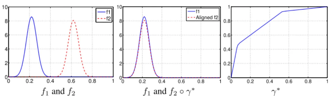
The optimization is performed using a numerical procedure called thedynamic programming algorithm. Fig. 1.1 shows an example of this alignment between two Gaussian density functions. After optimization, the two functions are nicely aligned, as shown in the middle panel, and the resulting optimal warpingγ∗is shown in the right panel.

0 0.2 0.4 0.6 0.8 1 0 2 4 6 8 10 f1 f2 0 0.2 0.4 0.6 0.8 1 0 2 4 6 8 10 f1 Aligned f2 0 0.2 0.4 0.6 0.8 1 0 0.2 0.4 0.6 0.8 1 f1andf2 f1andf2◦γ∗ γ∗

Figure 1.1 Alignment of two functions: alignf2tof1. The middle panel shows the aligned result.

−2 0 2 0.4 0.6 0.8 1 1.2 −2 0 2 0.4 0.6 0.8 1 1.2 0 0.2 0.4 0.6 0.8 1 0 0.2 0.4 0.6 0.8 1

Original functions{fi} Aligned functions{fi◦γi∗} γi∗’s

Figure 1.2 Multiple functions alignment. The leftmost panel shows a set of functions which have different height and peak locations. The middle panel shows the aligned result, and the right panel shows the optimal warping functionγi∗’s.

In case we have multiple functions that need to be aligned, we can extend the previous pairwise alignment as follows. We use the fact that the quantity in Eqn. 1.2 is actually a proper metric in a certain quotient space, and use it to define a mean function. This mean function serves as a template for aligning other functions, i.e. each function is aligned to this mean function. In fact, the problem of multiple alignment and mean computation are formulated and solved jointly using an iterative procedure: initialize the mean functionµand iteratively solve for

γi= arg inf γ∈Γkµ−(qi◦γ) p ˙ γk, i= 1,2,· · · , n,and µ= 1 n n X i=1 (qi◦γi) p ˙ γi . (1.3)

A synthetic example of multiple functions alignment is shown in Fig. 1.2. The leftmost panel shows a number of bimodal functions in which the heights and locations of peaks are different. The aligned functions are shown in the middle panel, and the optimal warping functionsγis are shown in the right panel.

Next we show one example of the multiple functions alignment in a real dataset: the Berkeley growth dataset which contains54female and 39 male subjects. To better illustrate,

0 5 10 15 20 0 5 10 15 20 25 30 0 5 10 15 20 0 5 10 15 20 25 30 0 5 10 15 20 0 5 10 15 20 25 30 Mean Mean+STD Mean−STD 0 5 10 15 20 0 5 10 15 20 25 30 0 5 10 15 20 0 5 10 15 20 25 30 0 5 10 15 20 0 5 10 15 20 25 30 Mean Mean+STD Mean−STD

Original data{fi} Aligned data mean±std, after

Figure 1.3 Analysis of growth data. Top row shows the growth data for54females, and the bottom row shows the growth data for39males.

we analyze the first derivatives of the growth curves. The results are shown in Fig. 1.3. Top row shows the alignment result for54female subjects and the bottom row shows the alignment result for39male subjects. The last column shows the mean±(cross sectional) standard deviation plot after the alignment. From the result, one can see that while the growth spurts for different individuals occur at slightly different times, there are some underlying patterns to be discovered.

1.3

Elastic Shape Analysis of Curves

The framework for function alignment can be easily extended to perform shape analysis of parameterized curves. Here the objects of interest are given by parameterized curvesf : [0,1]→_Rn_{. (Note that in case of closed curves it is natural to use}

S1as the parameterization domain, rather than an interval.) TheL2metric is given byhf1, f2i=

R1

0 hf1(t), f2(t)idtand the resulting normkf1−f2k=R

1

0 |f1(t)−f2(t)|

2_{dt, where| · |denotes the vector norm.} The mathematical representation of curves is in form of the square-root velocity function

(SRVF) given by Srivastava et al. (2011a) and Kurtek et al. (2012b):

q: [0,1]→Rn, q(t) = ˙ f(t) q |f˙(t)| .

The re-parameterization group here is the set of all positive diffeomorphisms of[0,1]. Ifq

is the SRVF of a curve f, then the SRVF of the re-parameterized curvef◦γ is given by

(q◦γ)√γ˙; we will denote this by(q, γ). Other simple representations of planar curves have been presented in Bauer et al. (2013).

f ◦γ1 γ1 f◦γ2 γ2

Figure 1.4 An illustration of re-parameterization curve in domainD= [0,2π].

From the perspective of shape analysis, a rigid motion (or translation), re-parameterization, rotation and scaling of a curve do not alter its shape. The translation has been removed by the SRVF representation automatically. An illustration of different parameterizations of a curve is shown in Fig. 1.4. The shape off is exactly the same as the shape off◦γ, for any

γ. The same holds for the rigid rotation of a curve. For anyO∈SO(n), the rotated curve

Of(t)has the same shape as the original curve. If we do not consider the scaling for the moment, this leads to formulation of equivalence classes, or orbits, of representations that all correspond to the same shape. Let[f]denote all possible translations, rotations and re-parameterizations of a curve f. The corresponding set in SRVF representation is given by

[q] ={O(q, γ)|O∈SO(n), γ∈Γ}. Each such class represents a shape uniquely and shapes are compared by computing a distance between the corresponding orbits.

As mentioned earlier, the SRVF representation satisfies the property thatkqk=k(q, γ)k, andkq1−q2k=k(q1, γ)−(q2, γ)kfor allγ∈Γand allq, q1, q2. Using this property, the shape distance between any two shapes is given by:

d([q1],[q2]) = inf

γ∈Γ,O∈SO(n)kq1−O(q2, γ)k=γ∈Γ,Oinf∈SO(n)kO(q1, γ)−q2k . (1.4) This optimization emphasizes the joint nature of our analysis – on the one hand we opti-mally register points across two curves using re-parameterization and rotation, and on the other hand we obtain a metric for comparing shapes of the two curves. The optimization overSO(n)andΓis performed using coordinate relaxation – optimizing over one variable while fixing the other. The optimization overSO(n)uses the Procrustes method while the optimization overΓuses the dynamic programming algorithm (Srivastava et al. 2011a). In absence of any other constraints on the curves, a straight line betweenq1and the registered

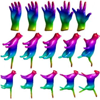
q2, i.e.O∗(q2, γ∗), with these quantities being the minimizers in the equation 1.4, forms the desired geodesic. However, if we rescale the curves to be of unit length or restrict ourselves to only the closed curves, then the underlying space becomes nonlinear and requires additional techniques for computing geodesics. We have developed a path-straightening algorithm for computing geodesics in the shape space of closed curves under the elastic metric, as described in Srivastava et al. (2011a). Fig. 1.5 shows some examples of geodesic paths between several pairs of closed curves taken from the MPEG7 dataset (Jeannin and Bober 1999). One can see that this joint framework deforms one shape to another in a natural way – the features are

Figure 1.5 Each row shows an example of geodesic path between the starting and ending shapes under the elastic framework.

better preserved across shapes and deformations are smooth.

Mean Shape and Modes of Variations: This framework is amenable to the development of tools for statistical analysis of shapes. For example, given a set of observations of curves, we may want to calculate the sample mean and modes of variations. Furthermore, we are interested in capturing the variability associated with the shape samples using probability models. The notion of a sample mean on a nonlinear manifold is typically defined using the Karcher mean (Karcher 1977). Let f1, f2, ..., fn be the observed sample shapes and

q1, q2, ..., qn be the corresponding SRVFs. The Karcher mean is defined as a quantity that satisfies: [µ] = argmin_[q]Pn

i=1d([q],[qi])2, whered([q],[qi])is calculated using Eqn. 1.4, andµ is the SRVF representation of the mean shapef¯. The search for the optimal mean shapef¯can be solved using an iterative gradient-based algorithm (Karcher 1977; Kurtek et al. 2012b; Srivastava et al. 2005). Fig. 1.6 shows some sample mean shapes calculated using this approach.

In addition to the Karcher mean, the Karcher covariance and modes of variation can be cal-culated to summarize the given sample shapes. Since the shape space is non-linear, we can use the tangent space at the mean shapeµ, which is a standard vector space, to perform the statistical analysis. We first map each sample shape onto the tangent space using inverse expo-nential map:vi= logµ(qi), then we define the covariance matrix to be:C=_n−1₁P

n i=1vivit. Using Principal Component Analysis (PCA) ofC, we can get the modes of shape variation. If PCk denotes the k-th principal direction, then the exponential mapexpµ(tPCksk)as a function oftshows the shape variation in PCkprincipal direction with standard deviationsk.

Figure 1.6 Mean shapes of four different classes of shapes. Each mean shape (shown in magenta color) is calculated from shapes on its left.

Fig. 1.7 shows the modes of variations for different classes of shapes in Fig. 1.6.

Statistical Shape Models: After obtaining the mean and covariance, the further step is to develop probability models to capture the distribution of given sample shapes. It is challenging to directly impose a probability density on the non-linear shape space. A common solution is to impose a distribution on a finite subspace of the tangent vector space. For example, one can restrict to principal subspace of the tangent space at meanµ. Then, we can impose a multivariate Gaussian distribution on the principal subspace with zero mean and covariance matrix obtained from the sample shapes. Fig. 1.8 shows the examples of random samples using means and covariance matrices estimated from shapes shown in Fig. 1.6.

While traditional shape analysis removes the transformations resulting from rigid motions and global scaling in shape considerations, in elastic shape analysis we additional remove the effects of re-parameterizations. In some situations, however, there is a need for removing other groups such as the affine and projective groups. For a discussion on the resulting affine-elastic shape analysis of planar curves, we refer the reader to the paper Bryner et al. (2014). This paper also describes a framework for projective-invariant shape analysis of planar objects but using point-set representations rather than continuous curves, using the ideas first proposed in Kent and Mardia (2012).

1.4

Elastic Shape Analysis of Surfaces

The task of comparing shapes of 3D objects is of great interest in many important applications. For instance, the shapes of anatomical parts can contribute in medical diagnoses,

S eco nd m o de First mode S eco nd m o de First mode S eco nd m o de First mode S eco nd m o de First mode

Figure 1.7 Modes of variations: for each class of shapes in mean shape examples (Fig. 1.6), we show the variation along the first and second principal modes. Shape in the center is the mean shape.

including monitoring the progression of diseases (Grenander and Miller 1998; Kurtek et al. 2011; Samir et al. 2014). The main challenge in such shape analysis comes from the fact that image data are often collected from different coordinate systems and data registration becomes a critical part of the analysis. In the following discussion, we will focus on surfaces that are embeddings of a unit sphereS2 inR3. In other words, the surfaces of interest can be parameterized using the sphere according to a mappingf :S2→R3. For anys∈S2, the vectorf(s)∈R3denotes the Euclidean coordinates of that point on the surface. The domain of interest is D=_S2_{, and the}

L2 metric is given by hf1, f2i=

R

S2hf1(s), f2(s)im(ds), withm(ds)denoting the Lebesgue measure onS2, and the resulting norm iskf1−f2k=

R

S2|f1(s)−f2(s)|

2_{m(ds). Let(u, v)denote the local coordinates of a points∈}

S2. Then, the vectors ∂f_∂u(s)and ∂f_∂v(s)span the two-dimensional space tangent to the surface at point

f(s)and

n(s) =∂f

∂u(s) × ∂f ∂v(s)

is a vector normal to the surface at f(s). Its magnitude |n(s)|=phn(s), n(s)i denotes infinitesimal area of the current parameterization at that point and the ration(s)/|n(s)|gives the unit normal vector. The mathematical representation of surfaces, suitable for elastic shape analysis, given by thesquare-root normal field(SRNF) defined as (Jermyn et al. 2012; Xie et al. 2013):

q:S2→R3, q(s) =pn(s)

|n(s)| .

The re-parameterization group here is the set of all positive diffeomorphisms of _S2_{. Ifqis} the SRNF of a surfacef, then the SRNF of the re-parameterized surfacef ◦γ is given by

(q◦γ)p

Jγ, whereJγis the determinant of the Jacobian matrix of the mappingγ:S2→S2. We will denote this by (q, γ). Similar to the identities presented for previous two cases, this representation also follows the isometry conditions: for all surfaces f, f1, and f2, and the corresponding SRNFs q, q1, and q2, and all γ∈Γ, we have:kqk=k(q, γ)k and kq1−q2k=k(q1, γ)−(q2, γ)k.

Once again, from the perspective of shape analysis, a re-parameterization and a rotation of a surface does not alter its shape. The shape offis exactly same as the shape ofO(f◦γ), for anyγ∈ΓandO∈SO(3). This motivates the formulation of equivalence classes, or orbits, of representations that all correspond to the same shape. Let[f]denote all possible rotations and re-parameterizations of a surfacef. The corresponding set in SRNF representation is given by[q] ={O(q, γ)|O∈SO(3), γ∈Γ}. Each such class represents a shape uniquely and shapes are compared by computing a distance between the corresponding orbits. Similar to curves, the joint registration and shape comparison of surfaces is performed according to:

inf

γ∈Γ,O∈SO(3)k

q1−O(q2, γ)k= inf γ∈Γ,O∈SO(3)k

O(q1, γ)−q2k . (1.5) While the optimization overSO(3)is relatively straightforward, the optimization overΓis much more difficult here than the curve case. We have developed a gradient-based approach that uses the geometry of the tangent space Tγid(Γ). It uses a set of vector fields that

incrementally deform the current grid on f2, so as to minimize the cost function given in Eqn. 1.5.

Similar to the case of constrained curves, the task of computing geodesics between any two registered surfaces is not trivial and requires a path straightening-algorithm (see Kurtek

Figure 1.9 Each row shows an example of geodesic between a pair of objects (the starting and ending shapes).

et al. (2012a)). More recently, Xie et al. (2014a) have developed an approximation that first computes a straight-line geodesic between any two registered surfaces in the SRNF representation space, and then inverts each point along this geodesic to obtain a geodesic in the surface space. For more details, we refer the reader to these papers.

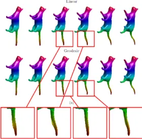
In Fig. 1.9, we show some examples of geodesics between objects including human hands and animals. In Fig. 1.10, we compare the geodesics between surfaces to the linear interpolation of surfaces. From the results, we can see that the tail part of the cat is distorted and inflated on the linearly interpolated path, but the tail part is better persevered along the geodesic path.

Using geodesics we can define and compute the mean shape using a standard algorithm for computing Karcher mean. Furthermore, we can define and compute Karcher covariance, and perform PCA on the tangent space at the mean shape. Figure 1.11 displays the observations and thek-th principal directions (PD) by constructing principal geodesicsexp_µ(tsk·PCk), where PCk ∈Tµ(F) is the kth principal component and sk denotes the corresponding standard deviation. The PDs are displayed using the triples{exp_µ(−sk·PCk), µ,expµ(sk· PCk)}. This analysis can be used to define a multivariate normal distribution on the principal coefficients and thus a random tangent vector from this Gaussian model. Assume that v

is a random deformation of the mean surface, i.e., v∈Tµ(F) according to the normal model. Then, we can use the shooting method to get a random sample of surfaces such that

Figure 1.10 Comparing geodesic to linear interpolation.

Observations

1st PD 2nd PD 3rd PD

Random Samples

Figure 1.11 Computing mean shape, PC analysis and random samples under a Gaussian model. The first row shows some observations of chess piece. The second row shows the three main principal components. And the last row shows several randomly sampled chess pieces using a Gaussian model.

1.5

Metric-Based Image Registration

In the problem of image understanding, especially in object recognition and classification using image data, it is important to perform registration of images during their analysis. The importance of image registration comes across clearly in many applications. For example, in developing image templates of different letters and numbers in human handwriting, for the purposes of automated handwriting recognition, it is important to align images of same objects before averaging. To improve performance, it is often necessary to perform a nonrigid alignment, i.e. deform one image so as to match its pixel patterns with the other image as much as possible. While these deformations have been performed using various energy minimization methods in the past (Beg et al. 2005; Bookstein 1989; Collignon et al. 1997; Davies et al. 2002; Dupuis and Grenander 1998; Eriksson and Astrom 2006; Joshi et al. 2004; Lorenzen et al. 2005; Miller et al. 2002; Szeliski and Coughlan 1997; Thirion 1998; Trouve 1998; Twining et al. 2004; Vercauteren et al. 2009; Viola and Wells III 1995), a novel idea is to use a proper metric for registration. As described in this section, there are several distinct advantages in this approach over the conventional ideas.

An image is treated as a function f :D→Rn, and the image space is F= {f :D→Rn | f ∈C∞(D)}. For a gray level image, we have n= 1, and for a colored image, we haven= 3. The domain of interest isD= [0,1]2_{, and the}

L2metric is given by hf1, f2i=R_Dhf1(s), f2(s)ids. LetΓ = Diff+(D)be a subgroup ofDiff+(the orientation-preserving diffeomorphism group) that preserves the boundary ofD. A registration of image

f1to imagef2is to find a diffeomorphismγ∈Γsuch that pixel valuesf1(s)andf2(γ(s)) are optimally matched to each other.

In the elastic framework, the mathematical representation of any image is given by a square-root map (SRM): q(s) =pa(s)f(s), where a(s) is the “generalized area multiplication factor” off ats∈D. It takes the forma(s) =|Jf(s)|_V where|Jf(s)|_V =

k_∂x∂f1 ∧

∂f

∂x2k. Here ∧denotes the wedge product, (x

1_{, x}2_{) :D→}

R2 are the coordinates on (a chart of) D andJf(s)is the Jacobian matrix off atswith the (j, i)-th element as

∂fj_/∂xi_{(s). The two special cases are: ifn= 2, thena(s) =|Jf(s)|; if and n= 3, then}

a(s) =k_∂x∂f1(s)×

∂f

∂x2(s)k. Note that this SRM by definition applies to images such that

n≥2. In case of gray level images, one can use their gradient images,(fu, fv)(s)∈R2, to fit into this representation. Intuitively, the SRM leaves uniform regions as zeros while preserving edge information in such a way that it is compatible with change of variables, i.e., stronger edges get higher values.

For f ∈ F and any γ, the SRM representation of f◦γ is given by (q, γ) =

p

|Jγ|(q◦γ). As mentioned earlier, under this representation, we have kqk=k(q, γ)k and k(q1, γ)−(q2, γ)k=kq1−q2k, for all q, q1, q2 and for all γ∈Γ. For the purpose of registration, we define an objective function between two images f1 and f2 by L(f1,(f2, γ)) =kq1−(q2, γ)k. The registration of two images is then achieved by minimizing the objective function according to:

γ∗= arginf

γ∈Γ

L(f1,(f2, γ)) = arginf γ∈Γ

kq1−(q2, γ)k , (1.6) The optimization problem overΓin Eqn. 1.6 forms the crux of our registration framework and is solved using agradient descentmethod as in Kurtek et al. (2010); Xie et al. (2012, 2014b).

This registration framework satisfies a list fundamental properties such as: (1) it is invariant to simultaneous warping; (2) it is inverse consistent (Xie et al. 2014b). Additionally, the optimal registration is not affected by scaling and translations of image pixels: let g1=c1f1+d1 and g2=c2f2+d2 with c1, c2≥0 andd1, d2∈Rn, if γ∗=

arg infγL(f1,(f2, γ))thenγ∗= arg infγL(g1,(g2, γ))as well.

In Fig. 1.12, we first present some results on synthetic images to demonstrate the use of the registration framework suggested in Eqn. 1.6. The imagesf1andf2are registered twice by first takingf1as the template image and estimatingγ21that optimally deformsf2using Eqn. 1.6. Then, the roles are reversed andf2 is used as the template to obtainγ12. We show the two converged energies,k(q1, γ12)−q2kandkq1−(q2, γ21)k, associated with the optimal

γ12 andγ21 to verify symmetry. The cumulative diffeomorphisms γ21◦γ12 andγ12◦γ21 are also used to demonstrate the inverse consistency of the proposed metric. The theory indicates thatγ12 andγ21 are expected to be inverses of each other. We show the original imagesf1andf2with the matching warped imagesf2◦γ21andf1◦γ12respectively. The diffeomorphismsγ12andγ21learnt to register the images are also presented. By composing them in different orders we expect the resulting diffeomorphisms to be the identity map. In order to better visualize that the composed diffeomorphisms are close to identity, we apply them to checkerboard images. We observe that the composed diffeomorphismsγ21◦γ12and

γ12◦γ21are close to the identity map.

f1 (f1, γ12) (f2, γ12−1) γ12 γ12◦γ21

f2 (f2, γ21) (f1, γ21−1) γ12 γ21◦γ12

Figure 1.12 Registering Synthetic Smooth Grayscale Images. γ12= arginfγ∈Γk(q1, γ)−q2k and γ21= arginfγ∈Γkq1−(q2, γ)k. kq1−q2k= 0.2312, kq1−(q2, γ21)k= 0.0728 and k(q1, γ12)−q2k= 0.0859.

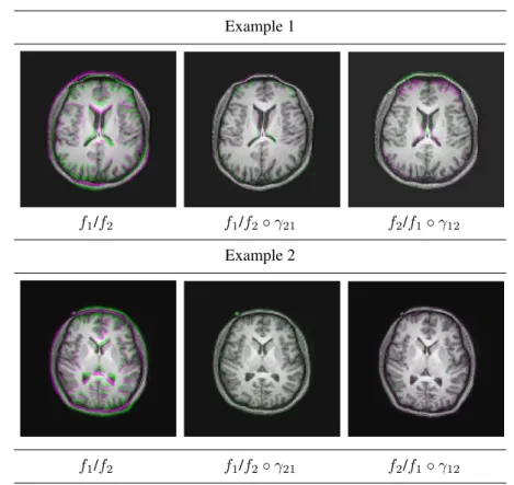
In Fig. 1.13, we present registration results using 2D brain MR images. In order to illustrate our method, in each of the two experiments, we show (1) the original images overlappedf1/f2and (2) overlapped images after registration (f1/f2◦γ21andf2/f1◦γ12). The overlapped images show image pairs in a common canvas.

Example 1

f1/f2 f1/f2◦γ21 f2/f1◦γ12

Example 2

f1/f2 f1/f2◦γ21 f2/f1◦γ12

Figure 1.13 Two examples of brain MR image registration (each row as an example). First column shows overlapped original imagesf1andf2; second column shows overlapped imagesf1and deformed

f2; third column showsf2and deformedf1.

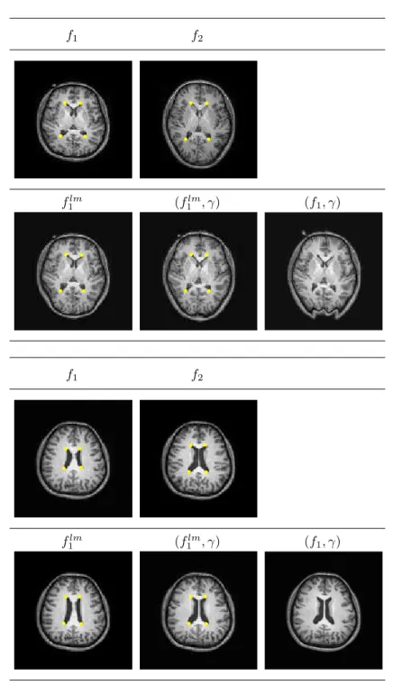
When objects in images have some specific landmarks, either provided by experts or some additional data analysis, they can provide some guidance in defining image correspondence. Automated registration methods routinely produce results that conflict with our contextual knowledge, and annotated landmarks provide a way to reconcile these two ideas. The framework can be further extended so that landmark information is incorporated during registration and all of the nice mathematical properties of the objective function are preserved.

Two pairs of 2D brain MR images are used to illustrate this procedure. In Fig. 1.14, we want to registerf1tof2. Four landmark points are provided and are displayed in each image as yellow dots. The images are first registered using only the landmarks, with a kernel based approach, and the resulting deformed image isflm

1 . We further deformf1lmby applying our registration method as in Eqn. 1.6 with restricted vector fields, specified by a set of basis so that the landmark pionts remain intact. The final result is shown as(f₁lm, γ)and are compared to registration without landmarks as f₁lm. The optimally deformed f1 without landmark information is displayed in the last column as(f1, γ)as a baseline. Since the deformation in the skull is so large that our method gives a local solution. By adopting the landmark-aided

registration, we at first get a deformed imageflm

1 , with the landmarks nicely matched and the skull deformed correspondingly. Thenflm

1 is further deformed to register the intensity details without moving the landmarks. The final result(flm

1 , γ)matchesf2with no artifacts around the skull. Generally, the registration with landmarks outperforms registration without landmarks.

1.6

Summary and Future Work

We have presented an overview of elastic shape analysis for several kinds of objects, including Euclidean curves, surfaces inR3, real-valued functions on[0,1], and 2D images. The analysis is characterized by a simultaneous registration of points across objects and comparisons of their shapes. The key idea is to restrict to parameterized objects and to use parameterization as a tool for registration under metrics that are invariant to all shape-preserving transformations, including re-parameterizations. The use of such metrics is facilitated by square-root mappings of original data because under these mappings, the original metrics become the standard L2 metric. For each of the data type considered, we present the corresponding square-root transformation and demonstrate some associated statistical tools.

In terms of future work, there are several questions associated with this framework that remain open. An important issue in choosing the elastic metric (or the related square-root representation) is the uniqueness. For instance, in the context of FDA and phase-amplitude separation, one can pose the question: Are there other transforms that allow, under the L2 metric, an appropriate framework for function registration? In fact, there exist other mappings, e.g.f(t)7→G(f(t),f˙(t))

q

|f˙(t)|, whereGis an arbitrary function off andf˙, that leads to isometry under theL2norm. However, their pros and cons in different situations needs to be explored further.

Another important area in shape analysis of curves is the groups beyond the similarity transformations. We have already mentioned the paper by Bryner et al. (2014) that provides affine-invariant shape analysis of elastic curves. However, such an elastic analysis of planar curves that is invariant under projective transformation group, remains to be developed.

References

Bauer M, Bruveris M and Michor PW 2013 R-transforms for SobolevH2_{-metrics on spaces of plane curves.eprint} arXiv:1311.3526.

Beg M, Miller M, Trouv´e A and Younes L 2005 Computing large deformation metric mappings via geodesic flows of diffeomorphisms.International Journal of Computer Vision61, 139–157.

Bookstein FL 1989 Principal warps: Thin-plate splines and the decomposition of deformations.IEEE Transactions on Pattern Analysis and Machine Intelligence11(6), 567–585.

Bryner D, Klassen E, Le H and Srivastava A 2014 2D affine and projective shape analysis.Pattern Analysis and Machine Intelligence, IEEE Transactions on36(5), 998–1011.

Collignon A, Vandermeulen D, Marchal G and Suetens P 1997 Multimodality image registration by maximization of mutual information.IEEE Transactions on Medical Imaging16(2), 187–198.

Davies R, Twining C, Cootes T, Waterton J and Taylor C 2002 A minimum description length approach to statistical shape modeling.IEEE Transactions on Medical Imaging21(5), 525–537.

Dryden I and Mardia K 1998Statistical Shape AnalysisWiley series in probability and statistics. Wiley.

Dupuis P and Grenander U 1998 Variational problems on flows of diffeomorphisms for image matching.Journal Quarterly of Applied MathematicsLVI(3), 587–600.

Eriksson A and Astrom K 2006 Bijective image registration using thin-plate splines. Pattern Recognition, International Conference on, vol. 3, pp. 798–801.

Grenander U and Miller MI 1998 Computational anatomy: An emerging discipline. Quarterly of Applied MathematicsLVI(4), 617–694.

Jeannin S and Bober M 1999 Shape data for the MPEG-7 core experiment ce-shape-1 @ONLINE.

Jermyn IH, Kurtek S, Klassen E and Srivastava A 2012 Elastic shape matching of parameterized surfaces using square root normal fieldsProceedings of the 12th European Conference on Computer Vision - Volume Part V, pp. 804–817, Berlin, Heidelberg.

Joshi S, Davis B, Jomier BM and B GG 2004 Unbiased diffeomorphic atlas construction for computational anatomy. Neuroimage23, 151–160.

Karcher H 1977 Riemannian center of mass and mollifier smoothing. Communications on Pure and Applied Mathematics30(5), 509–541.

Kent JT and Mardia KV 2012 A geometric approach to projective shape and the cross ratio.Biometrika99(4), 833–849.

Kneip A and Ramsay JO 2008 Combining registration and fitting for functional models.Journal of the American Statistical Association.

Kurtek S, Klassen E, Ding Z and Srivastava A 2010 A novel Riemannian framework for shape analysis of 3D objects Computer Vision and Pattern Recognition (CVPR), 2010 IEEE Conference on, pp. 1625–1632.

Kurtek S, Klassen E, Ding Z, Jacobson SW, Jacobson JB, Avison M and Srivastava A 2011 Parameterization-invariant shape comparisons of anatomical surfaces.IEEE Transactions on Medical Imaging30(3), 849–858. Kurtek S, Klassen E, Gore JC, Ding Z and Srivastava A 2012a Elastic geodesic paths in shape space of parameterized

surfaces.IEEE Transactions on Pattern Analysis and Machine Intelligence34(9), 1717–1730.

Kurtek S, Srivastava A, Klassen E and Ding Z 2012b Statistical modeling of curves using shapes and related features. Journal of the American Statistical Association107(499), 1152–1165.

Liu W, Srivastava A and Zhang J 2010 Protein structure alignment using elastic shape analysisProceedings of the First ACM International Conference on Bioinformatics and Computational Biology, pp. 62–70 BCB ’10. ACM, New York, NY, USA.

Liu W, Srivastava A and Zhang J 2011 A mathematical framework for protein structure comparison. PLOS Computational Biology.

Lorenzen P, Davis B and Joshi S 2005 Unbiased atlas formation via large deformations metric mapping InMedical Image Computing and Computer-Assisted Intervention MICCAI 2005(ed. Duncan J and Gerig G) vol. 3750 of Lecture Notes in Computer ScienceSpringer Berlin Heidelberg pp. 411–418.

Mardia KV and Dryden IL 1989 The statistical analysis of shape data.Biometrika76(2), pp. 271–281.

Miller M, Trouve A and Younes L 2002 On the metrics and Euler-Lagrange equations of computational anatomy. Annual Review of Biomedical Engineering4, 375–405.

Ramsay JO and Li X 1998 Curve registration. Journal of the Royal Statistical Society: Series B (Statistical Methodology)60(2), 351–363.

Ramsay JO and Silverman BW 2005Functional Data AnalysisSpringer Series in Statistics 2nd edn. Springer. Samir C, Kurtek S, Srivastava A and Canis M 2014 Elastic shape analysis of cylindrical surfaces for 3D/2D

registration in endometrial tissue characterization.Medical Imaging, IEEE Transactions on33(5), 1035–1043. Srivastava A, Joshi SH, Mio W and Liu X 2005 Statistical shape analysis: Clustering, learning, and testing.IEEE

Transactions on Pattern Analysis and Machine Intelligence27(4), 590–602.

Srivastava A, Klassen E, Joshi SH and Jermyn IH 2011a Shape analysis of elastic curves in Euclidean spaces.IEEE Transactions on Pattern Analysis and Machine Intelligence33(7), 1415–1428.

Srivastava A, Wu W, Kurtek S, Klassen E and Marron JS 2011b Registration of functional data using Fisher-Rao metric.arXiv:1103.3817v2.

Su J, Kurtek S, Klassen E and Srivastava A 2014 Statistical analysis of trajectories on Riemannian manifolds: Bird migration, hurricane tracking and video surveillance.The Annals of Applied Statistics8(1), 530–552.

Szeliski R and Coughlan J 1997 Spline-based image registration.International Journal of Computer Vision22(3), 199–218.

Tang R and Muller HG 2008 Pairwise curve synchronization for functional data.Biometrika95(4), 875–889. Thirion J 1998 Image matching as a diffusion process: an analogy with Maxwell’s demons.Medical Image Analysis

2(3), 243–260.

Trouve A 1998 Diffeomorphisms groups and pattern matching in image analysis.International Journal of Computer Vision28(3), 213–221.

Tucker J, Wu W and Srivastava A 2012 Analysis of signals under compositional noise with applications to sonar dataOceans, 2012, pp. 1–6.

Tucker JD, Wu W and Srivastava A 2013 Generative models for functional data using phase and amplitude separation.Comput. Stat. Data Anal.61, 50–66.

Twining C, Marsland S and Taylor C 2004 Groupwise non-rigid registration: The minimum description length approach.Proceedings of the British Machine Vision Converence (BMVC)1, 417–426.

Vercauteren T, Pennec X, Perchant A and Ayache N 2009 Diffeomorphic demons: Efficient non-parametric image registration.NeuroImage45(Supplement 1), S61–S72.

Viola P and Wells III W 1995 Alignment by maximization of mutual information Computer Vision, Fifth International Conference on, pp. 16–23.

Xie Q, Jermyn I, Kurtek S and Srivastava A 2014a Numerical inversion of SRNFs for efficient elastic shape analysis of star-shaped objectsEuropean Conference on Computer Vision (ECCV).

Xie Q, Kurtek S, Christensen GE, Ding Z, Klassen E and Srivastava A 2012 A novel framework for metric-based image registrationProceedings of the 5th International Conference on Biomedical Image Registration, pp. 276– 285 WBIR’12. Springer-Verlag, Berlin, Heidelberg.

Xie Q, Kurtek S, Klassen E, Christensen GE and Srivastava A 2014b Metric-based pairwise and multiple image registration2014 European Conference on Computer Vision (ECCV).

Xie Q, Kurtek S, Le H and Srivastava A 2013 Parallel transport of deformations in shape space of elastic surfaces 2013 IEEE International Conference on Computer Vision (ICCV), pp. 865–872.

f1 f2

f1lm (f1lm, γ) (f1, γ)

f1 f2

flm

1 (f1lm, γ) (f1, γ)

Figure 1.14 Two examples of brain image registration with landmarks. In each experiment, the top row shows the original imagesf1andf2, and in the bottom row, the first column shows the deformed imagesf1lmusing only landmarks; the second column shows the final deformed images(f1lm, γ)with

flm

1 as the initial condition; and the last column shows the registered images(f1, γ)without involving landmarks.