arXiv:1901.00778v1 [astro-ph.EP] 3 Jan 2019
Physics of Planet Trapping with Applications to HL Tau
A.J. Cridland
1,2⋆, Ralph E. Pudritz
2,3†, & Matthew Alessi
21Leiden Observatory, Leiden University, 2300 RA Leiden, the Netherlands
2Department of Physics and Astronomy, McMaster University, Hamilton, Ontario, Canada, L8S 4E8 3Origins Institute, McMaster University, Hamilton, Ontario, Canada, L8S 4E8
4 January 2019
ABSTRACT
We explore planet formation in the HL Tau disk and possible origins of the prominent gaps and rings observed by ALMA. We investigate whether dust gaps are caused by dynamically trapped planetary embryos at the ice lines of abundant volatiles. The global properties of the HL Tau disk (total mass, size) at its current age are used to constrain an evolving analytic disk model describing its temperature and density profiles. By performing a detailed analysis of the planet-disk interaction for a planet near the water ice line including a rigorous treatment of the dust opacity, we confirm that water is sufficiently abundant (1.5×10⁻⁴ molecules per H) to trap planets at
its ice line due to an opacity transition. When the abundance of water is reduced by 50% planet trapping disappears. We extend our analysis to other planet traps: the heat transition, dead zone edge, and the CO2 ice line and find similar trapping. The formation of planets via planetesimal accretion is computed for dynamically trapped embryos at the water ice line, dead zone, and heat transition. The end products orbit in the inner disk (R <3 AU), unresolved by ALMA, with masses that range between sub-Earth to 5 Jupiter masses. While we find that the dust gaps correspond well with the radial positions of the CO2, CH4, and CO ice lines, the planetesimal accretion rates at these radii are too small to build large embryos within 1 Myr.
Key words: protoplanetary discs, planetary migration, interplanetary medium
1 INTRODUCTION
What process or processes are responsible for the gaps and
rings structure in disks like HL Tau? A number of
expla-nations have been proposed including the existence gap-opening planets (Dipierro et al. 2015; Tamayo et al. 2015), efficient grain growth (Pinte et al. 2016), and sintering-induced grain fragmentation near ice lines (Zhang et al. 2015; Okuzumi et al. 2016). Rings of bright emission and the gaps between them are not restricted to HL Tau, and appear to be a common feature in protoplanetary disks (Zhang et al. 2016).
The correspondence between the gaps in the HL Tau disk and volatile ice lines (also known as condensation fronts) has been studied previously by Zhang et al. (2015). They used a temperature profile derived from a 2D radiative transfer model and assumed that ice lines would appear at the radii where the gas reached the sublimation temperature for a number of abundant volatiles. Zhang et al. (2016) go on to suggest a connection between ice lines, dust trapping, and emission gaps. Because dust trapping is an important
⋆ E-mail: [email protected]
† E-mail: [email protected]
first step in the process of planet formation, we might ex-pect that the first planetary seeds (often called planetary embryos), or up to fully formed planets may also be found in conjunction with the radial position of ice lines in these young systems.
The nature of this connection must take into ac-count the fact that planets exchange angular mo-mentum with their host disks and will migrate through them (Goldreich & Tremaine 1979; Ward 1997; Paardekooper et al. 2010). Linear solutions of the total torque on small (∼M⊕) planets suggest that their migration will occur in only 105 yr which is a small fraction of the disk
achieve masses of ∼10 Earth masses at which point they are liberated from their trap through the saturation of the corotation torque (see Cridland et al. (2016)) or through opening an annular gap in the disk. Both the saturation of the corotation torque and gap opening depend on the local gas viscosity, and hence on the ionization state of the gas. In this way, planet formation becomes linked to the position and movement of traps, as well as their microphysics over the full lifetime of the disk. This has been previously been shown by both analytic and numerical studies (see review by Pudritz et al. (2018)).
This raises two important questions about the nature of planet building and disk features in the HL Tau system. (1) What chemical species have ice lines that are capable of trapping planets? (2) Can planets also appear at the other traps? We note that while it has already been suggested that the water ice line acts as a trap (Lyra et al. 2010), do other species provide traps as well (eg. CO or CO2ice lines)?
Those that can, should harbour growing planetary embryos, which could create pressure maxima or even outright gaps in the disks. Those that cannot serve as traps would then be expected to only provide ring features arising from opacity transitions (Zhang et al. 2016). The answers to these ques-tions require that we are able to locate the posiques-tions of pre-dicted traps at the particular age of an observed star-disk system.
In this paper we address these two problems, specifi-cally; (1) what species are capable of trapping planets at their associated ice line radii in evolving disks, and (2) using our combined chemical and planet formation models where are the traps in the observed HL Tau disk and what mass planets - if any - might they harbour?
The water ice line is the archetype for planet trapping and works because its opacity transition modifies the disk’s temperature profile (Lyra et al. 2010; Dittkrist et al. 2014). Thus to address the first problem - what species can produce planet traps - we construct a general physical theory which analyzes the opacity transition across the water ice line by computing both the radial distribution of the ice from a photo-chemical disk model and the optical properties of an ice-silicate grain mixture. We generalize this theory to study planet trapping at the ice lines of other abundant volatiles like CO and CO2.
To accomplish these goals, we first generate HL Tau disk models that reproduce the global properties (mass, size, age) of the HL Tau disk. We tune our initial conditions so that after roughly 1 Myr of disk evolution one recovers the observed properties (ie. gas and dust mass, radial size) of the HL Tau disk. Then, using a complex photo-chemical code we compute the radial distribution of abundant volatiles (in their ice and gas phases) and find coincidence between the radial location of their ice lines with the observed gaps. We can also compute the growth of planetary embryos that can form at the ice line of abundant volatiles and elucidate the details of Type-I migration around the opacity transition induced by an ice line. These embryos would perturb the gas creating pressure maxima towards which the dust will flow, resulting in the observed gaps in emission (Dipierro et al. 2015).
To address our second question - what planets might have formed in the current HL Tau disk - we investigate planet formation in HL Tau by applying models that we
have developed in Cridland et al. (2016, 2017a,b) to our HL Tau disk models. This planet formation model combines the standard planetesimal accretion model (Kokubo & Ida 2002; Ida & Lin 2004) with a planet trap model to limit the inward migration rate of the proto-planet (Masset et al. 2006; Hasegawa & Pudritz 2013) within the predicted disk age of 1 Myr. We also generalize our analysis of planet trap-ping to the other planet traps (heat transition, Lyra et al. (2010); Horn et al. (2012) and dead zone, Matsumura et al. (2009); Reg´aly et al. (2013)) that have appeared in our pre-vious formation models.
We derive the radial locations of ice lines by computing the photo-chemistry of our evolving analytic disk model, and compare their locations to the radial locations of the gaps observed today, and to the results of Zhang et al. (2015). We define the location of the ice line to be the point where the ice abundnace exceeds the abundance of the correson-ponding vapour. This definition has served well in the past in thermochemical equilibrium calculations (eg. Alessi et al. (2017)) where the transition from vapour to ice is very sharp. It is important to note that in light of our more complete treatment of the astrochemistry, the transition between wa-ter vapour and ice can be (radially) slow, and in the case of water spans roughly 4 AU in our model (see Figure A2). In this case a better definition for the ‘location’ of the ice line would be where the abundance of the volatile ice exceeds half of its total abundance.
We note that models of ‘pebble accretion’ show that the growth of a planetary core may be dominated by the ac-cretion of cm-sized ‘pebbles’ rather than 10-100 km sized planetesimals (Lambrechts & Johansen 2014; Bitsch et al. 2015). Pebble accretion as a formation mechanism for rocky planetary cores is an active field of research. However, recent numerical studies have suggested that the direct accretion of pebbles onto a planetary core is limited to only∼1 M⊕ because the pebbles are ablated in the planetary envelope (Brouwers et al. 2018) and are then recycled back into the surrounding protoplanetary disk (Alibert 2017). The effi-ciency of this recycling is not well constrained by hydrody-namic simulations. In 2D and 3D simulations Ormel et al. (2015a) and Ormel et al. (2015b) find that only 1% of the envelope mass per orbital time is filtered back into the disk, while Lambrechts & Lega (2017) and Fung et al. (2015) find 10% and 100% respectively. Given these current uncertain-ties, our work continues for now, to focus on planetesimal accretion for the growth of planetary embryos.
2 MODEL BACKGROUND
Our theoretical framework is an ‘end-to-end’ analysis that links the structure and evolution of an accretion disk down to the formation and growth of a young planet. This frame-work combines an analytic gas disk model, a numerical dust physics model, a Monte Carlo radiative transfer scheme, a time-dependent astrochemical code, and a planet formation model to ultimately compute the chemical composition of the gas that is delivered to the atmosphere of a growing planet (for technical details see Cridland et al. (2016) and Cridland et al. (2017a)).
A similar method has been developed by Mordasini et al. (2016) (and reviewed in Mordasini (2018)) which they call a ‘chain’ model. The chemical evolution of the gas is not computed in their model, and volatile abundances were either prescribed by observational data, or removed entirely. In this way, the majority of elements heavier than helium were accreted onto planets as ice frozen to planetsimals. Mordasini et al. (2016) do, however, compute the final equilibrium structure and molecular abundances of the resulting planetary atmosphere - something that is beyond the scope of this work.
In our framework, the models that govern physics and chemistry are computed in succession. The ordering of our calculations begins with the prescription of a gas model for an evolving disk. The following steps are: gas disk model
→dust model (radial drift, growth / fragmentation) →UV
/ X-Ray radiative transfer →time dependent chemistry→
planetesimal accretion planet formation. Each step, much
as in the chain model, depends on the preceding ones, and impact the results of all following ones. In doing this we can successively model complicated interactions like the impact of dust evolution on the radiative transfer of high energy radiation (see Cridland et al. (2017a)).
Any particular model in this scheme acts as an input for all subsequent calculations, while it has no impact on models that it follows. One such example is the existence and evolution of the turbulent dead zone (which depends on the ionization, computed in the chemistry step) should, in principle impact the settling and fragmentation of large dust grains. However the ionization depends on the flux of ionizing radiation, and hence on the distribution of the dust grains. This could in principle be solved by iterating
thedust model→rad transfer→chemistrysteps, however
this is computationally expensive. Additionally we showed in Cridland et al. (2017a) that such a calculation has a min-imal impact on the radial extent of the dead zone.
2.1 Gas disk model
The details of our model are outlined in Cridland et al. (2016), Cridland et al. (2017a), and Alessi et al. (2017), and we refer readers to those papers for the technical details. Here we will summarize some of its most important fea-tures. The gas disk model is a self-similar, analytic model as seen in Chambers (2009). It computes the co-evolving radial structure of the gas surface density and midplane tempera-ture as mass viscously accretes through the disk. The radial structure follows a power law of the form:
Σ(r, t)∝Σ0(t)r
−p T(r, t)∝T
0(t)r
−q, (1)
where the exponentspandq are determined by the source of gas heating and the time dependent functions Σ0 and
T0 depend on the mass accretion rate, and hence on our
choice ofαin the standard α-disk prescription of the disk viscosity (Shakura & Sunyaev 1973). In what follows we as-sume a diskα= 10−3, their functional form can be found
in Chambers (2009).
We note here that historicallyα was used to describe the strength of gas turbulence in the disk - leading to mo-mentum transport and hence accretion. However recently (in light of the existence of dead zones, see below)αhas been used simply as a parameterization of the rate of accretion through the disk. In past work (see Cridland et al. (2017b) and Alessi et al. (2017)) we assume two components of an-gular momentum transport: turbulence and magnetic disk winds - each contributing to maintain a constant (in time and space) ‘diskα’:
α=αturb+αwind. (2)
Such a distinction becomes important when including the effects of a turbulent dead zone on the dynamics of the dust disk (discussed below).
There are two primary heating sources in an accretion disk, viscosity and direct irradiation. The former is ulti-mately caused by the conversion of gravitational potential energy into heat as the gas accretes through the viscous disk, while the latter is caused by the absorption and re-emission of stellar radiation by the upper atmosphere of the disk. Generally speaking, viscous heating dominates the inner re-gion of the disk, while direct irradiation becomes important at larger radii.
At a certain radius, the radiative heating becomes more important than the heating from viscous evolution. We call this radius the heat transition (rt), so generally the surface
density and temperature of the gas is given by:
Σ Σ0
(r)∝
(
r−3/5 r < r
t
r−15/14 r > r
t
(3)
T T0
(r)∝
(
r−9/10 r < r
t
r−3/7 r > r
t
. (4)
As the mass accretion rate drops, viscous heating is less efficient and rt moves inward. Eventually the temperature
structure is fully determined by direct irradiation, similar to the results of Chiang & Goldreich (1997).
In light of our above assumption that the effectiveα
associated with angular momentum transport can be gener-ated by both turbulence or magnetic winds, we note that the effective viscosity responsible for heating in the inner disk is generated by both the Reynolds (turbulent) stress and Maxwell (magnetic) stress. Hence upon entering the dead zone (whereαturbfalls by at least two orders of magnitude),
heating is dominated by non-ideal MHD effects (eg. ambipo-lar diffusion heating) which, in steady state theory heats the disk at a rate that scales with the release of gravitational po-tential energy (Ciesla & Cuzzi 2006; Bai & Stone 2013).
We assume that the disk α stays constant through-out the disk, and that the functional form of the viscos-ity (ν=αcsH) remains the same regardless of the primary
the relevant length scale will still be related to the gas scale height (H). Then the effectiveαis related to the ratio of the magnetic pressure to the gas pressure, as well as the local orientation of the magnetic field (Bai & Stone 2013).
One drawback of using an effective viscosity to handle both turbulent and MHD disk wind torques is that while the former leads to radial outward spreading of the disk, winds transport carries away angular momentum leading to shrink-age of the disk (Pudritz & Norman 1986). Indeed, in recent models that include non-linear MHD effects, the spread of the disk is suppressed (Bai 2016). This probably will not effect he dynamics in the inner, planetary forming regions of the disk.
2.2 Dust model
The dust is allowed to evolve separately from the gas, and its evolution depends on the level of coupling between a dust grain and the gas. The parameter which describes this coupling is known as the Stokes number - the ratio of the grain stopping time to eddy turnover time:
St= aρs Σ
π
2, (5)
whereais the radius of the grain,ρsis the internal density
of the grain, and Σ is the gas surface density. WhenSt <1 the grain is well coupled to the gas and will primarily evolve with the viscous evolution of the gas. While when St > 1 the dust will decouple from the gas and orbit the host star in Keplarian orbits. Because the gas is pressure supported and orbits at sub-Keplarian speeds the large grains will feel a head wind as they pass through the gas. This head wind drains angular momentum and moves the grain into smaller orbits. This process is known as radial drift (Weidenschilling 1977), and proceeds on a time scale of:
τdrif t= rVk
Stc2
s
γ−1, (6)
whereVkis the Kepler speed,csis the gas sound speed, and
γ is the absolute magnitude of the gas pressure gradient. Radial drift plays an important role in our model because it impacts both the radial structure of the dust, which changes the flux of high energy radiation (Cridland et al. 2017a), and provides ample solid material for the formation of planetesi-mals at small radii (Dr¸a˙zkowska et al. 2016; Cridland et al. 2017b). It does, however, clear out the solid material at large radii, and makes planet formation through the accretion of planetesimals more difficult at radii outward of the water ice line.
Along with its radial drift, the dust can coagulate, fragment, and settle. Each of these processes depend sen-sitively on the level of turbulence in the gas (see for ex-ample Dullemond & Dominik (2005), Birnstiel et al. (2009), and Birnstiel et al. (2012)) which we assume is a constant
αturb= 10−3 in most of our calculations. Such an
assump-tion relies on a consistent source of turbulence that is of-ten attributed to the magnetorotational instability (MRI) (Balbus & Hawley 1991).
Non-ideal magnetohydrodynamic (MHD) calculations (Bai & Stone 2011; Simon et al. 2013; Bai & Stone 2013, 2017) have suggested that along the midplane of the disk the MRI is suppressed by either Ohmic diffusion or the Hall
effect - often called a ‘dead zone’. In this laminar flow, angu-lar momentum transport is dominated instead by a launch-ing of a magnetize wind (Pudritz et al. 2007; Bai & Stone 2011; Simon et al. 2013). We stress that while the turbu-lent component of the angular momentum transport may drop within the dead zone, the MHD disk wind maintains the transport of angular momentum required to remain in a steady state disk solution (constantα= 10−3).
For the disk models discussed in§3 we assume a con-stantαturbwhen computing the evolution of the dust.
How-ever in§5, where the goal is to demonstrate the physics of planet trapping at the dead zone edge we will vary αturb
according to the method outlined in Cridland et al. (2017a) (see also Appendix C).
Within the dead zone of varied turbulent alpha model the gas ionization (as computed by our chemical model dis-cussed below) is too low for turbulence to be efficiently gen-erated by the MRI (Bai & Stone 2011). With the only source of turbulence generated through hydrodynamical sources, the turbulentαturbdrops significantly. Here we assume that
within the dead zoneαturb= 10−5while outward of the dead
zone edge αturb = 10−3. With the reduction in turbulent
power the relative speed of the dust grains is reduced. This reduces the efficiency of fragmentation, which leads to larger grains that can more effectively settle to the midplane of the disk. This is due to both the grains being larger (heavier) and the reduction of turbulence that would otherwise mix grains back up above the midplane.
2.3 Ionizing radiation
We compute the transfer of UV and X-Ray radiation because of its importance on the astrochemistry in protoplanetary disks (Fogel et al. 2011). We use the Monte Carlo radiative transfer schemeRADMC3D(Dullemond 2012) to compute the flux of photons through out the disk. To properly model the flux from a T Tauri star we compute the radiative trans-fer for four wavelengths within a range of 930-2000 ˚A for UV and 1-20 keV for X-Rays. We then extrapolate the re-maining wavelengths within the above ranges using a sample spectrum as seen in Fogel et al. (2011) and Bethell & Bergin (2011). These sample spectra have been normalized to match the total flux from TW Hya, and can be scaled if needed.
2.4 Disk astrochemistry
The astrochemistry is computed with a time-dependent gas chemistry code as featured in Fogel et al. (2011), Cleeves et al. (2014), and Cridland et al. (2016). Generally it computes the reaction rates of many (∼5900) chemical re-actions including gas phase, volatile absorption/desorption on grains, grain surface reactions (for the production of H2O
and H2), and photo-chemistry. We allow for the chemical
Each snapshot includes gas density and temperature profiles, a dust density profile, and the UV and X-Ray radi-ation fields. As the disk ages, each of these profiles change from one snapshot to the next. Each snapshot begins with the same molecular initial condition and is run until a steady-state solution is found. This method allows the chem-istry to be computed in parallel over many snapshots simul-taneously, which dramatically reduces the required comput-ing time.
The chemical model is initialized with molecular abun-dances based on observations of the volatile component of molecular clouds. Of particular importance, water is initial-ized as an ice with an abundance of 1.5×10⁻⁴ molecules per
H-atom. This abundance is used as our fiducial water abun-dance model used below. While also assuming that the dust follows the typical gas-to-dust mass ratio of 100 we find a maximum water ice-to-silicate mass ratio of about 0.13 out-ward of the water ice line and approximately zero inout-ward of the water ice line.
Within the ice line the water ice smoothly transitions between these two mass ratios. Our fiducial mass ratio re-sides at the lower end of the ice mass ratio inferred from the comet 67P/C-G by Davidsson et al. (2016). Similarly it is lower than the three test cases of Bitsch & Johansen (2016)1 who computed a similar test of the impact of the
water ice abundance on planet migration. Our choice of wa-ter abundance is based on general knowledge of the global astrochemical properties of protoplanetary disks.
The reaction rates that are used to compute the adsorp-tion and desorpadsorp-tion of volatiles are based on lab measure-ments of ice binding strengths, and hence have associated uncertainties. We have not propagated these uncertainties through our calculation of the ice lines radial location (see below), and hence we can not estimate the uncertainties in the radial location of the ice lines. Additionally we assume that all ice is pure when it desorbs - which ignores the des-orption of clathrate hydrates (as explored by Zhang et al. (2015)), mixes of water ice with trapped gaseous molecules. These species of water ice generally have lower sublimation temperatures than pure water ice, and hence could produce additional ice lines or shift the location of the ice lines that are computed below.
2.5 Planet formation and migration
Our planet formation model follows the standard planetesi-mal accretion model (Kokubo & Ida 2002; Ida & Lin 2004), where the core of a young planet is built by the successive accretion of∼10-100 km sized objects. Core growth is seeded with a mass of 0.01 M⊕, and is largely insensitive to the ini-tial embryo mass because the accretion timescale scale with the mass of the core (Ida & Lin 2004).
In these semi-analytic models, accreting protoplanets are assumed to grow from planetesimals within a feeding zone of approximately 10 Hill radii (rH =a(Mp/3M∗)1/3). For a planetesimal to accrete its speed relative to the pro-toplanet should be:σ/Ω∼10rH (Ida & Lin 2004). However
this prescription generally ignores the combined impact of migration and gravitational scattering of planetesimals by
1 the lowest of which was a 0.33 ice-to-silicate mass ratio
the protoplanet (for ex. Tanaka & Ida (1999)). In practice, the accretion of planetesimals within the feeding zone may not be completely efficient. The effect of this inefficiency is beyond the scope of this work, and we assume that all plan-etesimals within the feeding zone are available for accretion. We combine this accretion model with the dynamical trapping of forming planets in ‘planet traps’ to limit the rate of Type-I migration. Planet traps slow the Type-I mi-gration rate of proto-planets because of a combination of the Lindblad and co-rotation torques which can reverse the di-rection of angular momentum transport (Masset et al. 2006; Hasegawa & Pudritz 2011).
Specifically, planet traps are discontinuities in the phys-ical properties of the disk which causes the direction of the net torque acting on the planet to reverse direction. In past works, the three planet traps which we focussed on were the water ice line, the heat transition, and the outer edge of the dead zone. The discontinuities associated with these traps are the dust opacity, gas temperature profile, and gas tur-bulence strength respectively. In this work we model these discontinuities and compute the net torque on a planet at each of these traps and demonstrate their influence on plan-etary migration.
We note that, for simplicity, the models for these dis-continuities (ie. transition in turbulent strength) have not been accounted for in computing the radial structure of the gas and dust. In most cases, these discontinuities change the structure of the disk locally, near the planet trap, and do not have an impact on the global structure and overall evolution of our disk model. In past works we have verified that a change in the turbulent strength does not drastically change the global distribution of the dust which act as a primary source of opacity for high energy photons (see the appendix of Cridland et al. (2017a)). As a result the ioniza-tion structure, and hence the size and evoluioniza-tion of the dead zone is not changed when its physical effect on the disk is included in our model.
In our model we assume that the planet is trapped at one of the planet traps, and migrates only because the location of the planet trap changes as the disk ages. This assumption remains valid as long as the co-rotation torque remains unsaturated (Paardekooper et al. 2010; Hasegawa & Pudritz 2013). The saturation of the co-rotation torque occurs mainly when the gas turbulence is weak, and so at each timestep we check the saturation of the co-rotation torque if the planet trap is found within the dead zone (see below).
If the co-rotation torque saturates, the planet migrates due to the standard Lindblad torque Paardekooper et al. (2010):
Γ =CΓΣΩ2pr
4
p
Mp
M∗
2
rp
|∆r|
2
, (7)
whererp, Ωp,Mp, andM∗are the radial position, Keplar fre-quency, mass of the planet, and host star mass respectively. |∆r| is the relavent length scale for the density gradient, which we set as the maximum of the disk scale height (H) or the Hill radius (RH). The radial evolution of the
proto-planet is ˙rp/rp= Γ/Jpsuch that:
1
rp
drp
dt =−
CΓΣΩpr2p
Mp
Mp
M∗
2
rp
max(H, RH)
2
The numerical constant CΓ is related to the strength of
the net torques on the planet (ie. see Paardekooper et al. (2010)).
When the planet is sufficiently massive (few tens of M⊕), its gravitational tug on the surrounding gas will over-power the viscous torques and open a gap in the gas disk. At this point Type-I migration is suppressed and the planet be-gins Type-II migrating. In this regime, the planet migrations inward on the viscous timescale, as it acts as an intermedi-ary to angular momentum transport through the disk. In this case the orbital radii of the planet evolves as:
1
rp
drp
dt =− ν r2
p
, (9)
whereνis the gas viscosity, andν=αcsH for the standard
‘α-disk’ (Shakura & Sunyaev 1973).
2.6 Verifying the process of planet trapping
Our previous analysis of co-rotation torque saturation as-sumed that the process was discrete, so that the co-rotation torque saturates only after the planet reached a particu-lar mass (computed by comparing the eddy-turnover rate and libration rate, see Cridland et al. (2016)). However Paardekooper et al. (2011a) showed that this process ac-tually occurs as a smooth transition between the satura-tion states of the co-rotasatura-tion torque. This smooth transi-tion is captured by a set of three numerically motivated functions that weaken the co-rotation torque in regions of the disk where we would have otherwise assumed that it was fully unsaturated. The full form of the total torques that were derived by Paardekooper et al. (2011a) was used by Coleman & Nelson (2014) to compute the global rate of Type-I migration over their entire disk and across a wide range of planetary masses. In §4 we follow the method of Coleman & Nelson (2014) to compute the trapping of plan-ets near volatile ice lines, the heat transition, and the dead zone edge.
One purpose of this paper is to verify that planet trap-ping proceeds near the designated planet traps that are out-lined in previous works (Cridland et al. 2016; Alessi et al. 2017). This is done by computing the total torque on a planet as was done in Coleman & Nelson (2014), and re-quires a modification to our original disk model that cap-tures the physics responsible for planet trapping.
In the case of the ice line this requires a modified disk model where the dust opacity is allowed to change as a function of radius across the ice line. For this model, we assume that the bulk of the solid mass is made up of only 0.1µm sized grains with an ice mantle that varies with ra-dius. Hence we take the radial distribution of water ice from previous astrochemical results and compute the resulting optical properties of the dust-ice mixture. The details and results of these calculations are outlined in Appendix A and §4 respectively. The purpose of this calculation is to show how a change in the dust opacity due to changing water ice abundance leads to a reversal of the net torque near the ice line.
We expect that trapping at the dead zone is related to the distribution and size of dust grains which impact the opacity, and hence temperature profile of the gas. This as-sumes the gas and dust temperatures are equal, which is
the case at for high densities along the midplane. To test whether the dead zone acts as a trap we compute the den-sity and size distribution of the dust using the numerical model of Birnstiel et al. (2012), then compute the temper-ature profile of this dust population using the Monte Carlo
code RADMC(Dullemond 2012). In computing the
radia-tive transfer we are forced to neglect the radial distribution of water ice in order to keep the calculation tractable. We assume that the solid component is made up of (water) icy grains everywhere. In this case we focus primarily on the physical processes that result in planet trapping near the dead zone.
We combine this radiative temperature profile with the viscous temperature profile that we compute analytically to get the total gas temperature profile by summing their en-ergy densities, such that:T4
gas,total=Tviscous4 +Tradmc4 . The
details of these calculations are outlined in§4 and appendix C.
2.7 Evolution of HL Tau’s Disk
For our purpose of testing the possibility of planet forma-tion in HL Tau, we wish to use a disk model whose proper-ties resemble those of the HL Tau disk. Generally the disk parameter that can most easily be tuned to match observed properties is the initial mass of the disk. Unfortunately since most Class-II systems are up to a few Myr old, this is impos-sible to constrain observationally for any individual system. Instead we pick disk models with initial masses that evolve to have the same mass as is observed in the HL Tau disk at an age of∼1 Myr. We used the stellar parameters outlined by White & Hillenbrand (2004), and a total dust mass of (1-3)×10−3 M
⊙(Carrasco-Gonz´alez et al. 2016) to estimate a total gas mass of 0.1-0.3 M⊙assuming a global gas-to-dust ratio of 100. Assuming that the disk is 1 Myr old then its initial gas mass must have been 0.25-0.63 M⊙ according to the evolution of our gas disk model. Thus, to account for the range of disk masses, we run three models with initial masses of 0.25 M⊙, 0.44 M⊙, and 0.63 M⊙, that we define as the ‘low-mass’, ‘mid-mass’, and ‘high-mass’ models re-spectively. These initial disk masses agree with the results of disk formation in star formation simulations carried out by Bate (2018)
Table 1.Model parameters between the four disk models. Also shown is the gas surface density and temperature at 105 yr and 1 AU,
as well as the global mass accretion rate through the disk at 105yr.
Name Mdisk,0 LU V Σ0(t= 105yr, r= 1AU) T0(t= 105yr, r= 1AU) M(˙ t= 105yr)
M⊙ LU V,T W Hya g/cm2 K Msol/yr
low-mass (LM) 0.25 100 1040 628 2.4×10⁻⁸
mid-mass (MM) 0.44 100 1565 847 4.9×10⁻⁸
high-mass (HM) 0.63 100 2135 1024 8.1×10⁻⁸
low-flux (LF) 0.63 1 2135 1024 8.1×10⁻⁸
possible exception is the CO ice line which resides at large radii (r >60 AU) for all disk models.
The reported UV flux of HL Tau (Bitner et al. 2008) is approximately 100× the observed flux from TW Hya (Yang et al. 2012). So we therefore scale the UV spectrum by a factor of 100 in our radiative transfer scheme. To facil-itate comparison to our past work, where we assumed the total UV flux was the same as TW Hya in all models, we ran a second high-mass model where we do not scale the UV spectrum. We summarize the varied parameters in Table 1.
3 RESULTS: THE POSITIONS OF ICE LINES AND OTHER TRAPS IN HL TAU
We compute the evolution of the gas and dust surface den-sity and temperature throughout the lifetime of the disk. These evolving profiles change the location of the ice lines as the disk cools and the surface density of material drops, particularly inward of the heat transition.
In Figure 1 we compare the radii of the condensation fronts for abundant volatiles in our chemical model and heat transition radius at 1 Myr in each of our disk models to the locations of the dust gaps in HL Tau as reported by Tamayo et al. (2015).
Generally we find that the CO2is located closest to the
inner gap, with CH4and NH3close to the second gap. In the
high-mass and low-flux models the CO2ice line is more
coin-cident with the inner gap than the lower mass models. This difference is due to the higher temperatures in the high-mass and low-flux models, attributed to a higher mass accretion rate and more efficient heating from viscosity. This difference in accretion rates also results in the shifted location of the heat transition between each of the models. Finally in the region of the disk that is primarily heated by direct irradi-ation (outward of the heat transition) there is no difference in the location of the CO and NH3 ice lines. Because the
temperature structure is independent of the amount of ma-terial outward of the heat transition when the disk is heated by direct irradiation.
The freeze out of pure CO occurs at the same radius (∼73 AU) in each of our models, and is located near the fourth gap. Another abundant volatile, N2never produces a
‘traditional’ ice line in our model - where the frozen phase becomes more abundant than the gas phase. However its ice phase reaches a maximum at ∼ 90 AU in each of the models. Because its sublimation temperature is generally slightly lower than CO, its clear that photo-chemical effects
like photo-desorption are suppressing the freeze out of N2,
pushing its ice line far from the host star.
The coincidence of the dust gaps and condensation fronts has been previously discussed in Zhang et al. (2015) who used the temperature profile 665(r/AU)−0.6K to
deter-mine the radial location of the ice lines. This profile was de-rived by a 2D radiative transfer model designed to model the observed SED of the HL Tau system (Men’shchikov et al. 1999). At 1 Myr the temperature profile in our high-mass disk model is 630(r/AU)−0.9 K when r < r
t and
24(r/40AU)−0.42 K whenr > r
t. We see that in our model
the gas is almost always cooler than the model used by Zhang et al. (2015), other than very near (r <0.8 AU) to the host star. This results in our disagreement of which ice lines are more coincident with the gap locations (see below). Zhang et al. (2015) report that the location of the inner two gaps correspond to the water and hydrated NH3ice lines
respectively. They report the start of a large outer gap at the CO2ice line and is centered on the sublimation temperature
of a combination of CO and N2on a water ice mantle. This
large gap spans the radii between the third and fourth gap reported by Tamayo et al. (2015) and used here. The fifth gap is not represented in Zhang et al. (2015).
An important distinction between the results of Zhang et al. (2015) and our own work is that they consid-ered the freeze out of hydrated species of volatiles, as well as the freeze out of volatiles on already established icy mantles - resulting in higher binding energies, and hence higher sub-limation temperatures than pure volatile freeze out. This extra layer of complexity is generally not included in as-trochemical simulations, and could cause small radial shifts in the location of the ice line. Since we model the tempo-ral evolution of the disk, any small shift in radius becomes equivalent to uncertainty in the system age.
0 20 40 60 80
Di
sk
r
ad
iu
s
(A
U
)
rgap, 1 = 13.6 AU
rgap, 2 = 33.3 AU
rgap, 3 = 65.1 AU
rgap, 4 = 77.3 AU
rgap, 5 = 93.0 AU
H2O CO2 CH4 CO
NH3
Heat transition
LM
(a) low-mass model
0 20 40 60 80
Di
sk
r
ad
iu
s
(A
U
)
rgap, 1 = 13.6 AU
rgap, 2 = 33.3 AU
rgap, 3 = 65.1 AU
rgap, 4 = 77.3 AU
rgap, 5 = 93.0 AU
H2O CO2 CH4 CO
NH3
Heat transition
MM
(b) mid-mass model
20 40 60 80
Di
sk
r
ad
iu
s
(A
U
)
rgap, 1 = 13.6 AU
rgap, 2 = 33.3 AU
rgap, 3 = 65.1 AU
rgap, 4 = 77.3 AU
rgap, 5 = 93.0 AU
H2O CO2 CH4 CO
NH3
Heat transition
HM
(c) high-mass model
20 40 60 80
Di
sk
r
ad
iu
s
(A
U
)
rgap, 1 = 13.6 AU
rgap, 2 = 33.3 AU
rgap, 3 = 65.1 AU
rgap, 4 = 77.3 AU
rgap, 5 = 93.0 AU
H2O CO2 CH4 CO
NH3
Heat transition
LF
(d) low-flux model
0.1 1.0
t (Myr)
0 20 40 60 80 100
R
ad
iu
s
(A
U)
HL_Tau_LM
(a) low-mass model
0.1 1.0
t (Myr)
0 20 40 60 80 100
R
ad
iu
s
(A
U)
HL_Tau_MM
(b) mid-mass model
0.1 1.0
t (Myr)
0 20 40 60 80 100
R
ad
iu
s
(A
U)
0.8 Myr
HL_Tau_HM
CH4 NH3 H2O N2O CO CO2 HT
(c) high-mass model
0.1 1.0
t (Myr)
0 20 40 60 80 100
R
ad
iu
s
(A
U)
HL_Tau_LF
(d) low-flux model
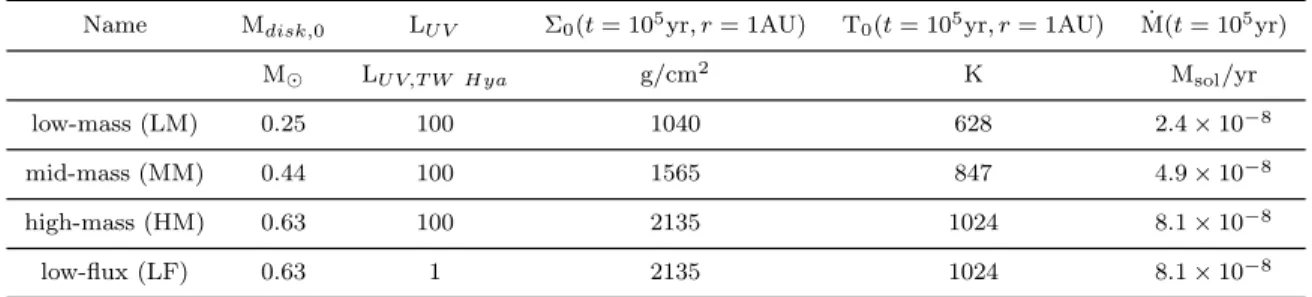
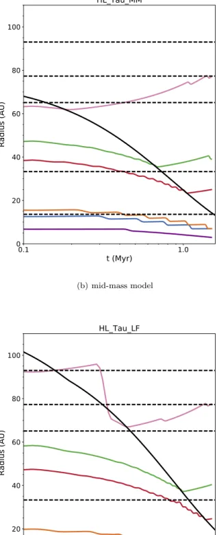
Figure 2. Temporal evolution of the ice line location in each of the presented disk models. We find that in the high-mass model there is a coincidence between the location of the CO2, CH4ice lines with the inner two gaps at a disk age of∼0.8 Myr (marked by a vertical
Note an outward motion for ice lines that cross the heat transition (black curve). Once an ice line is outward of the heat transition it exists in a region of the disk that has no evolution in its temperature profile - because heating is dominated by (an assumed) constant radiation field. As the surface density of the disk drops, photodesorption begins to impact the desorption rates of ice species, pushing the ice line outward.
By following their temporal evolution, we look for an epoch when the ice lines best agree with the location of gaps in the disk, as an additional method of estimating the system age. The ice line evolution is largely determined by the thermal evolution of the gas disk, and hence is given by the analytic disk model that we use. As a result, the high-mass and low-flux models have identical ice line evolution since their disk started with the same initial mass. In what follows we will exclusively discuss results as they apply to the high-mass model while implying that all conclusions can similarly be applied to the low-flux model.
Both the high-mass and mid-mass models show an in-stance when multiple ice lines coincide with the gaps. These epochs occur at ages of∼0.8 Myr and∼0.4 Myr respec-tively. Because the latter age is unreasonably small for the HL Tau system, and since the former age lies closest to the assumed age of the HL Tau disk (∼1 Myr) we will favour the disk parameters of the high-mass model in our analysis of planet trapping at ice lines.
4 RESULTS: PLANET TRAPPING AT ICE
LINES
The process of planet trapping at ice lines is driven by an opacity transition which locally changes the power law index of the temperature and gas density profiles. To sufficiently change the opacity across an ice line, one would expect that the volatile must be abundant. Water is an excellent candi-date for trapping because of its abundance and because its low average density has a strong effect on the total opacity of the solids when it freezes out (see Miyake & Nakagawa (1993) and Appendix A). Here we demonstrate planet trap-ping due to the opacity transition at the water ice line by modelling the freezes out of water as a function of radius across the ice line, and computing the resulting temperature profile for a viscously heated disk. In what follows we will use the stellar and disk parameters used in the ‘high-mass’ disk model at the epoch of highest coincidence between ice line and gap locations (t∼0.8 Myr), unless otherwise spec-ified. This model will act as our fiducial model, and provide a base from which we build our modified disk model (see below).
To assess the impact of the water ice line on the total torques on a planet we have added a much deeper treatment of opacity effects to our earlier work. It is based on the ana-lytic solutions of Chambers (2009), and used in our previous work (Cridland et al. 2016). This new enhanced (denoted ‘modified’) model takes the radial distribution of water ice from our previous astrochemical results (see Figure A2) as an input to compute the change in dust opacity (and subse-quent temperature profile) across the ice line using details of grain properties. In particular our opacity model depends on the mass abundance of ice that has accumulated on the grain
0.1 1.0 10.0 100.0
Disk
Radiu (AU)
10
100
1000
10000
T(K
) o
r Σ
g(g
/cm
3
)
Modified Di k Model
Fiducial model Ga temperature
Surface density
Figure 3.The gas temperature and surface density profiles for the modified disk model used to illustrate planet trapping. The initial temperature profile was taken from the ‘high-mass’ model at t = 0.8 Myr and denoted as ‘Fiducial model’.
- a property that depends on disk radius across the ice line. The details of this calculation are presented in Appendix A. Above a temperature of 1380 K, where dust is expected to sublimate, we return the prescription of the temperature depended opacity as discussed in Chambers (2009).
Our method of deriving the radial dependence of the icy dust opacity differs from other theoretical efforts like Bell & Lin (1994) or Stepinski (1998) (among others). In these works, the opacity is described by a power-law of tem-perature and density over different temtem-perature ranges, de-pending on the dominant physical effect generating the opac-ity (Bell & Lin 1994). These power-laws are fit or compared to tabulated values2 and the transition between
tempera-ture regions are either smoothed (Bell & Lin 1994; Stepinski 1998) or not (Bailli´e et al. 2016).
In this work we combine the tabulated opacities of bare silicates and pure water ice into a single Planck mean opacity using the method described by Miyake & Nakagawa (1993) (also see Appendix A). This method computes the effective complex spectral index for a mixture of ice and dust over a range of wavelengths. The relative abundance of ice and dust is set by our astrochemical disk model and depends on radius. These indices are then used to compute the total opacity using the internal opacity calculator of RADMC3D (for more details see Appendix A). In this way we can control the impact of a radially changing abundance of water ice without having to assume any power-law functional form for the temperature dependence in the opacity.
In Figure 3 we show the resulting midplane temperature and surface density profiles for the modified disk model. The ice line is within the viscously heated region of the disk, and the resulting drop in opacity allows for more efficient cool-ing. Therefore, the midplane temperature profile becomes slightly shallower within the ice line before returning to a slightly steeper power-law outward of the ice line. Because the accretion rate is constant in steady state disk theory,
0.1 1.0 10.0 100.0
Disk Radius (AU)
−4 −3 −2 −1 0 1 2 3 4
To
ta
l T
or
qu
e
(Γ0
)
Total Torque on a 1 M⊕ Planet
HT Water
ice line trap
Figure 4.Total torque acting on a 1 M⊕planet in our modified disk model normalized by Γ0. A strong positive total torque
ap-pears at the ice line, signifying trapping, while a strong transition appears near the heat transition (HT, vertical dashed line).
this restricts the surface density profile (see Appendix A). One might worry that these modifications might effect the thermal stability of the disk. We tested the Rayleigh stabil-ity of the disk (e.g. Yang & Menou (2010))3 and find that
our modified disk model does not harm the thermal stability of the disk.
We note that this modified disk model has a similar radial dependence inward of the ice line for both the perature and density as in our fiducial disk model. The perature profile steepens outside of the ice line as the tem-perature of the gas and dust is reduced, then eventually flat-tens as heating from direct irradiation becomes dominant. The disk is truncated at its maximum radius (∼ 112 AU at t = 0.8 Myr) in line with our previous work which does not include an exponential taper. This maximum radius is determined by the viscous spreading associated with the in-ward mass flux through the disk (see Chambers (2009) for details).
The dust opacity is higher inward of the ice line so the cooling is less efficient resulting in a higher temperature at low radii. In principle these higher temperatures will shift the location of the water ice line outward in the disk. How-ever this shift is small and does not effect the total torque on a planet. This model includes the change of the temper-ature radial profile at the heat transition, where gas heating becomes dominated by radiative processes rather than vis-cosity (outside of R∼ 30 AU). This is discussed in more detail below.
In Figure 4 we show the total torque acting on a 1 M⊕ planet in our modified disk model. The total torque includes both the Lindblad torques as well as the co-rotation torques, and were computed using the same method as Coleman & Nelson (2014), based on the work of Paardekooper et al. (2011a) (see Appendix D for a brief
3 The Rayleigh stability requiresV2
k +
1
r∂r∂
r3
ρ ∂P∂r
>0, where
P =ρc2
s/γ is the gas pressure,ρis the gas volume density, and
V2
k =GM∗/ris the square of the Kepler speed
0.1 1.0 10.0 100.0
Disk Radius (AU)
Γto
t
/Γto
t
,m
ax
Total Torque - Adjusting Water Abundance
[H2O]=[H2O]0 × 1.00
[H2O]=[H2O]0 × 0.65
[H2O]=[H2O]0 × 0.41
[H2O]=[H2O]0 × 0.25
HT Water
ice line trap
No trapping
Figure 5.Variation in the maximum water ice abundance rela-tive to the fiducial water abundance. After a drop of about half of the ice abundance the planet trapping signature disappears.
summary). The total torque is normalized by:
Γ0= (q/h)2Σgr4pΩ
2
p (10)
whereq=Mp/M∗andh=H/rp. The strong positive torque
at the ice line signifies the trapping that would occur there, and is determined by the change in the temperature profile across the ice line. We note the fiducial location of another assumed planet trap, the heat transition (vertical dashed line).
Also noted in Figure 4 is the location of the heat tran-sition (HT) - where the disk heating trantran-sitions from being dominated by viscosity to being dominated by the direct ir-radiation of the host star. At the heat transition there is also evidence for planet trapping, where the total torque transi-tions from positive to negative. This confirms our previous assertion (see for ex. Cridland et al. (2016)) that the heat transition should act as a planet trap.
It is noteworthy that there is another null point in the total torque between the ice line and heat transition traps. It can be shown that this null point is actually unstable, and rather represents a position from which a planet would be repelled rather than trapped.
4.1 Varying Water Ice Abundance
0 5 10 15 20 25 30 35 40
Disk Radius
(AU)
02 4 6 8 10 12 14
Du
st
op
ac
ity
(c
m
2
/g)
Variation of opacity across the ice line
[H2O]=[H2O]0 × 1.00
[H2O]=[H2O]0 × 0.65
[H2O]=[H2O]0 × 0.41
[H2O]=[H2O]0 × 0.25 IL
Figure 6. Radial dependence of the dust opacity for the four cases with varying maximum water abundances. The opacity drop at the water ice line is less severe as the maximum water abun-dance is reduced, hence the ability of the ice line to trap planets is reduced. We note the location of the water ice line (where the water ice abundance exceeds half of its maximum abundance in the fiducial model) with a dashed line.
trapping switches off when the water abundance drops be-low roughly half of the maximum water abundance from the fiducial model.
This result differs from those of Bitsch & Johansen (2016), who found no such reduction of planet trapping for a drop in abundance of an order of magnitude. However here we begin with a lower ice-to-silicate mass ratio, implying that the ice-to-silicate ratio must be below at least about 10% before seeing such an effect.
This result implies that volatiles that are less abun-dant than about half of the water abundance from the fiducial model will not produce planet traps at their ice line. Additionally our result implies that protoplanetary disks that either inherited low abundances of water, had their water destroyed early in their evolution (ie. the reset model of Eistrup et al. (2016)), or during the collapse stage (Drozdovskaya et al. 2016) could have less efficient planet trapping at their water ice line.
In Figure 6 we show the radial dependence of the dust opacity over the disk (up to a radius of 40 AU) as computed in Appendix A. We see why in Figure 5 the trapping disap-pears as the water abundance drops - because the reduction of opacity is less severe across the ice line as the water ice abundance is reduced. Hence for ice species with spectral features similar to water and abundances half that of water (in our fiducial model), we would not expect a sufficiently high opacity drop to lead to planet trapping.
Because of the multiplicity of ice lines in the HL Tau system, an interesting question arises: can the ice lines of other volatiles also act as planet traps? Below we test both CO2, which is much less abundant than water in our model;
and CO which is as abundant but resides in a part of the disk that is heated through irradiation (rather than viscosity).
0.1 1.0 10.0 100.0
Disk Radius (AU)
−4 −3 −2 −1 0 1 2 3 4
To
ta
l T
or
qu
e
(Γ0
)
Total Torque on a 1 M⊕ Planet
HT CO2 IL
Figure 7.Total torque on a 1 M⊕ massed planet for the case where dust opacity is determined by the abundance of CO2 ice
on water ice-covered dust grains. We additionally note the CO2
ice line (CO2IL) and the heat transition (HT). Here we show the
results for the high-mass model at a time of 0.1 Myr rather than our fiducial time of 0.8 Myr, hence the heat transition is farther out than in previous figures.
4.2 Planet Trapping at the CO2 Ice Line?
In Figure 7 we show the total torques around the CO2 ice
line (CO2 IL) for a 1 M⊕ mass planet. Similar to the case of the water ice line, the opacity transition at the CO2 ice
line causes a strong positive torque. We similarly see planet trapping near the heat transition (outer dashed line), how-ever it is shifted slightly with respect to the true location of the heat transition. This shift comes from the details of the modified disk model around the CO2ice line, which predicts
a slightly warmer disk than was computed for the disk model which varied water ice abundance. As a result the location of the heat transition in this disk model is shifted outward slightly.
In our model CO2in under-abundant compared to H2O
by a factor of about 400, so at first glance, it is surprising given above that a planet can be trapped at its ice line. Further analysis, however, shows that in the modified disk model the temperature profile of the gas is steepening near the CO2 ice line and hence even a relatively small
(com-pared to the effect of water) change to the dust opacity from the freeze out of CO2 flattens the temperature profile
enough to lead to planet trapping. In other chemical models (Drozdovskaya et al. 2014; Walsh et al. 2014; Eistrup et al. 2016) CO2 is more abundant, because they include dust
grain surface reactions which lead to its efficient formation, or because CO2 is inherited by the disk and not efficiently
destroyed. In these models the opacity transition would be stronger, further supporting the role of the CO2 ice line as
a planet trap.
4.3 Planet Trapping at the CO Ice Line?
The only other molecule that has similar abundances to H2O
irradi-ation by the host star, we require further analysis than is presented in this section to determine if it can indeed trap planets.
The above analysis assumes that the ice line resides in a region of the disk where heating is dominated by viscous dissipation. For the case of the CO ice line however, which lies at radii&30 AU, the disk gas will be primarily heated through the direct irradiation of the host star. Because of this we search for the effect of trapping by computing the temperature profile numerically with a Monte Carlo radia-tive transfer scheme.
In particular we search for a similar form of the temper-ature profile arising from the change in dust opacity across the CO ice line as was seen in the viscously heated part of the disk, leading to planet trapping. To test the validity of trapping planets at the CO ice line we similarly compute the dust opacity as a function of radius, starting from a mixture of silicate-water ice and adding CO ice with mass abundances given by the results of our previous astrochemi-cal simulations (see Cridland et al. (2017b) for an example). We follow the same method as before to compute the Planck mean opacity of the dust-ice mixture as a function of radius across the CO ice line (see Appendix A).
To assess the impact of changing the opacity across the CO ice line in a radiatively heated disk we compute the dust temperature of the dust using the radiative transfer
codeRADMC3D(Dullemond 2012). The underlying density
of the dust and gas are computed assuming solely viscous heating, and a constant gas-to-dust ratio. Hence the tem-perature computed numerically represents the excess heat available to the dust from stellar radiation, above the effect of viscous heating. For this calculation we simulated 20 dust populations which each have a varying abundance (relative to the number of hydrogen atoms) of CO ice between zero and 2.4×10⁻³. Each dust grain is the same size (0.1 µm)
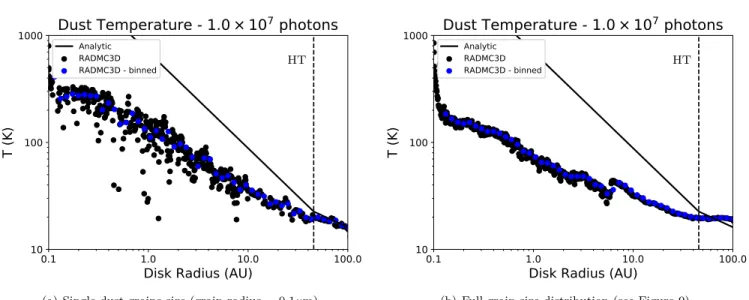
and we used 10 million photon packets withRADMC3D. In Figure 8 we compare the midplane dust tempera-ture profiles derived by RADMC3D(ie. radiative heating, points), and our analytic model (eqs. 3 and 4, solid). As expected, the dust temperature computed by RADMC3D
recovers the radial dependence of our analytic model out-side of the heat transition (rt, dashed line). While within
the heat transition we find that the dust temperature is consistently lower than is expected by viscous heating. This conclusion is consistent with the assumption of our analytic model as described by Chambers (2009), which asserts that within the heat transition (rt) the dust heating is dominated
by the heat released by the viscous evolution of the gas. We investigate two dust models and their consequences on the heating of the outer disk, and trapping at the CO ice line. The first is that the dust mass is dominated by the smallest (0.1µm) grains. Such an assumption overesti-mates the total dust opacity in the inner (r < rt) region of
the disk which causes the scatter observed in Figure 8(a). In principle this scatter would be reduced by the diffusive properties of the radiation field (which is not modelled by
RADMC3D), and is similarly reduced when the numerical
data is binned (blue points). For our second case, we com-pute the full dust size distribution using a Two-pop model (Figure 8(b), also see Figure 9). The bulk of the dust mass is in mm-sized grains, and the total dust opacity throughout
the disk is lower. Hence along the midplane the scatter in the dust temperature is lower (see Figure 8(b)).
In Figure 8(b) we show the dust temperature derived
by RADMC3D using the dust distributions computed by
the Two-population model. Near the dead zone edge we find a short positive gradient in the radiative temperature gra-dient (points). Likewise, outside of the heat transition the flattened temperature profile is a result of the enhancement of medium and small grains in the outer parts of the disk.
As mentioned above, we compute the temperature dial profile of the disk by combining both viscous and ra-diative heating profiles. To do this, we first bin the nu-merical data into 50 radial bins (blue points in Figure 8) spaced evenly in log-space over the rangeR∈[0.1,100]AU, and compute the average temperature within each bin (blue points). Next we add the energy densities which result from the viscous and radiative heating (aT4
vis and aTrad4
respec-tively), such that the final gas temperature is:
Ttot= Tvis4 +Trad4
1/4
, (11)
where Tvis is given by our analytic model (case r < rt
in equation 4), andTrad is given by the binned numerical
data). This combination assumes that the dust and gas are in thermal equilibrium, which is a reasonable assumption along the midplane of the disk. Such a combination pro-duces a temperature profile similar to the analytic model plotted in figure 8(a), but smooths the transition between viscous and radiative heating. As before, we compute the associated surface density profile assuming that the global mass accretion rate through the disk is constant in space ( ˙M = 3πνΣ), and the viscosity is given by the standard
α-disk model (ν=αc2
s/Ω).
We find no reversal in the direction of the net torque, and hence there is no trapping at the CO ice line. The lack of trapping comes from the fact that the dust opacity is not greatly reduced (factor of order unity) as CO freezes onto the grains. The opacity transition is therefore insufficient at the CO ice line to produce a strong positive net torque.
We have shown that the inner two gaps lie near the CO2
and CH4 ice lines and that CO2 is sufficiently abundant in
our model to lead to the trapping of a 1 M⊕planet. However, the CO ice line does not show evidence of planet trapping because the freeze out of CO does not constitute a large enough reduction in dust opacity (factor order unity) to lead to a perturbed temperature profile in the radiatively heated part of the disk. The CH4 ice line is similarly located near
the heat transition where, along with its low abundance we do not expect it to exhibit planet trapping. The third and fourth gaps surround the location of the CO ice line, however it is unlikely that these features are due to a planet trapped at the CO ice line.
5 RESULTS: A GLOBAL PICTURE OF
PLANET TRAPPING
5.1 Including the dead zone and heat transition
0.1
1.0
10.0
100.0
Disk Radius (AU)
10
100
1000
T (
K)
Dust Temperature - 1.0×10
7
photons
Analytic RADMC3D
RADMC3D - binned HT
(a) Single dust grains size (grain radius = 0.1µm)
0.1
1.0
10.0
100.0
Disk Radius (AU)
10
100
1000
T (
K)
Dust Temperature - 1.0×10
7
photons
Analytic RADMC3D
RADMC3D - binned HT
(b) Full grain size distribution (see Figure 9)
Figure 8.Comparison between different dust distribution models, and their resulting dust temperature fromRADMC3D. Solid line: midplane dust temperature based on our analytic model. Inward of the heat transition (dashed line) the disk is heated by viscous heating, while beyond the heat transition the midplane is heated by radiative heating. Points: midplane dust temperature from radiative heating alone computed byRADMC3D(black) as well as the binned data used in torque calculations (blue). The left figure is used in§4.3 while the right figure is used in§5. The difference in scatter between the two points is related to a net loss of opacity in the right figure when the bulk of the dust mass is allowed to grow from 0.1µm (left) to predominately mm-sized grains (right, also see Figure 9).
planet traps are the dead zone edge and the heat transition, representing a transition in the turbulentα(αturb) and
pri-mary gas heating source respectively.
Trapping at the dead zone edge has been attributed to a rising midplane temperature profile caused by the efficient settling of grains (Hasegawa & Pudritz 2010). The increase in solid density blankets the midplane from outgoing radi-ation, producing a positive temperature gradient. Likewise, the heat transition trap results from a change in the tem-perature gradient due to radiative heating at the midplane becoming more efficient than viscous heating (ie the second term in equation 11 becoming larger than the first).
As before, these trapping mechanisms depend on the temperature profile of the disk. However in this section the interplay between the radial distribution of the dust and the radiation field is more important than the radial distribution of the ice. Hence we replace our previous assumption of the dust grain population being dominated by a single grain size for a semi-analytic description of the surface density of grains with different sizes. For simplicity, and since the bulk of the disk is exterior to the water ice line, we keep the dust opacity constant in the disk during the Monte Carlo calculation of the dust temperature. Furthermore, since the water ice line is in the viscously heated part of the disk we do not see a strong contribution to the temperature profile from radiation (for example see Figure 8(a)), hence changing the opacity across the ice line will not have a large impact on the dust temperature.4.
We combine the Two-population dust model outline in Cridland et al. (2017a) (based on Birnstiel et al. (2012) and Birnstiel (2016)) with RADMC3Dto compute a new
tem-4 We assume that the grains are all covered by layer of water ice,
with a constant average opacity ofκ= 3 cm2/g
perature profile and the resulting total torques around the dead zone edge and heat transition.
In the Two-population model the coagulation, fragmen-tation, diffusion, and radial drift of dust is computed numer-ically using two representative dust populations - resulting in the total dust surface density radial profile. Then the surface density radial profile for a range of dust sizes are re-constructed using semi-analytic expressions which describe the average evolution of the grains as a function of their size. We implemented the evolution and implication of the dead zone in the Two-population model in a similar way as in the Appendix of Cridland et al. (2017a) (also see Appendix C in this work).
In Figure 9 we show the surface density profile for grains of different sizes. The location of the dead zone edge (3 AU), water ice line (6 AU), and heat transition (45 AU) are marked with vertical dashed lines. Inward of the ice line, the ice sublimates leaving grains that are more susceptible to fragmentation. This destroys the large grain population (a&1 cm) as they radially drift across the ice line.
In the outer region of the disk the size of the dust grains is limited by radial drift, the rate of which is dependent on the gas pressure gradient (and hence on the gradient of the gas temperature). The temperature profile steepens across the heat transition from larger to smaller radii as the disk heating becomes dominated by viscous evolution, resulting in a slower radial drift rate. We find that this change in the drift rate results in an enhancement for medium sized (a ∼0.01 cm) grains.
0.1
1.0
10.0
100.0
Disk Radius (AU)
0.0001
0.001
0.01
0.1
1
10
100
Σ
dust(g
/cm
2
)
Dust Surface Density
0.0001 cm 0.0100 cm 1.0000 cm 10.0000 cm
DZ IL
HT
Figure 9.Dust surface density radial profile for varying dust sizes attage= 0.8M yr. We mark the location of the outer dead zone
edge (DZ), ice line (IL), and heat transition (HT) with vertical dashed lines, located at∼3, 6, and 45 AU respectively.
position in the disk, up to the gap opening masses in our disk model. Again, in computing the temperature profile of the disk we combine the effects of viscous and radiative heating by taking the sum in equation 11, and use our modified model from section 4 to represent the temperature profile in the viscously heated part of the disk.
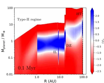
We find strong trapping near the water ice line (∼ 6 AU), as well as clear trapping (inward migration outward of the trap and outward migration inward of the trap) at the dead zone edge (∼3 AU) for 0.1 M⊕ . Mplnt . few
M⊕. By inspection the location of the dead zone trap in Figure 10(b) and the increase in the temperature profile in Figure 8(b) do not align, which disagrees with our previous assertion for the root cause of planet trapping at the dead zone. Instead it appears that the change of αturb is more
important to the net torque. This could be caused by the fact that at low turbulent viscosity (although high enough for the co-rotation torque to remain unsaturated) the co-rotation torque is primarily given by the horseshoe drag, rather than the linear torque (Paardekooper et al. 2011b). The strength of the horseshoe drag torque has a strong dependence in its entropy component to the temperature gradient, and hence with the steep temperature gradient in our viscously heating regime the horseshoe drag can overpower the outward torque of the Lindblad torque.
Approaching the heat transition from larger radii where the temperature profile flattens, the magnitude of the inward torques are strongly reduced. We find planet trapping at the heat transition for a range of larger masses than is seen for the dead zone and water ice line. This shift could be caused by the higher turbulent viscosity at the lower disk temper-atures near the heat transition, which tends to smooth out horseshoe orbits unless the planet is sufficiently massive. This result shifts the mass range where trapping is relevant to slightly higher masses than was assumed in our previ-ous work (Hasegawa & Pudritz 2013; Cridland et al. 2016; Alessi et al. 2017). However, the inward migration rate is still an order of magnitude lower than would be expected from standard Type-I migration, for planets with M<0.5
M⊕. Hence their migration is sufficiently slow that they have enough to time to grow into a mass range where they are effectively trapped.
While a heat transition null point does not appear for low mass planets, nevertheless it will act as aneffectivetrap. This effective trap reduces the migration rate enough to al-low for the growth of a super-earth core, at which point it will be fully trapped. The implications of this effective trap-ping can be studied through population synthesis models, and is left to future work. One particularly important ques-tion is whether a planet migrating due to the torques in Figure 10(b) will deviate far from a planet that is assumed to be perfectly trapped at the heat transition - since both scenarios result in similar migration timescales (factor of or-der unity). In our formation model below we assume that the planet is perfectly trapped at the heat transition.
5.2 Time Evolution of Global Trapping
We now show how the radial positions of these planet traps change as the disk ages. In our analytic model the disk evolves in two ways: 1) As mass accretes onto the host star the total mass of the disk decreases, reducing both the sur-face density of the gas and dust at all radii as well as reduc-ing the global mass accretion rate. 2) With the fallreduc-ing mass accretion rate, viscous heating becomes less predominant, lowering the temperature of the gas within the heat transi-tion. Thus the radial position of the heat transition moves inward because the temperature of the gas due to direct ir-radiation is not susceptible to the same time evolution. With the reduction of the gas and dust surface density, the flux of ionizing photons to the midplane of the disk increases, shrinking the dead zone.
In Figures 10(a) and 10(c) are formatted the same way as Figure 10(b), for an early (0.1 Myr) and late (1.9 Myr) time respectively. At early times the heat transition is not yet present because the disk heating is completely domi-nated by viscosity. It is also hotter and more dense at these early times which starts the ice line feature (now located at 8 AU) and dead zone edge (now located at 17 AU) farther out than they are observed later on in the disk’s lifetime, as seen in Figure 10(b) at 0.8 Myr. Nevertheless we see similar features at this early time as we saw above. The ice line trap has a mass range for trapping that is shifted to lower mass from what we saw in Figure 10(b). This can be attributed to it sitting within the dead zone early on in the disk’s life, while the dead zone has crossed it by 0.8 Myr. The dynami-cal implications for planets trapped at crossing planet traps is an interesting problem that is currently beyond our scope of work.