Rajasekar
In recent years, bike sharing systems ushered in the explosive growth. The growth of bike sharing systems brings both health benefits and environmental benefits.This study is a data analysis project that investigate the usage pattern of bike sharing system using Citi Bike open source data. This study studied the influence of weather and date on the bike usage, and compare the characteristic usage pattern of two different gender group. Based on that, this study provide a bike demand prediction and user gender prediction model. Also, with the comparison on usage of NY taxi, this study analysed when people prefer Citi Bike and verify that Citi Bike can be an ideal alternative transportation to taxi.
Headings:
Data Analysis
Information Visualization
by Yawei Tang
A Master’s paper submitted to the faculty of the School of Information and Library Science of the University of North Carolina at Chapel Hill
in partial fulfillment of the requirements for the degree of Master of Science in
Information Science.
Chapel Hill, North Carolina April 2018
Approved by
Table of Content
1. Introduction...3
1.1 Public bike sharing System...3
1.2 Background of Citi Bike... 4
2. Literature Review...6
3. Data Preparation and Feature Extraction... 9
3.1 Data Collection... 9
3.2 Data Cleaning...11
3.3 Data Visualization...12
4. Demand Analysis...15
4.1 Methods...16
4.1.1 Lasso Regulation used on Generalized Regression Model...17
4.1.2 K-means Clustering Method...18
4.2 Experimental Results... 19
4.2.1 Generalized Linear Regression...19
4.2.2 Clustering Model... 22
5. Gender Prediction... 24
5.1 Method... 26
5.2 Experimental Result...27
6. Comparison between the usage of Citi Bike and NYC Cab... 30
6.1 Data Cleaning and Feature Extraction... 31
6.2 Comparison on Average Speed...32
6.3 Comparison on Usage pattern...34
7. Discussion...37
8.Conclusion... 39
Bibliography... 41
1. Introduction
1.1 Public bike sharing System
Bikes are important part of public transportation since they are environment-friendly, cheap and easy to adapt to different environment. They also provide a popular form of recreation, and have been adapted for use as children's toys, general fitness and military and police applications. Nowadays, with the emphasis on healthy living style, bikes become even more popular. The bike sharing systems (also known as BSS) provide people an opportunity to use bicycles anytime and anywhere without the limitation of inconvenience (Parkes et al., 2013). People initially tried and failed to introduce
bike-sharing schemes in the 1960s due to the technical limitations such as tracking bikes and instant payment. However, nowadays, technological advances, such as bike tracking, solar powered sensors, mobile phones and wide-area internet and online aces, have helped transform bike-sharing from an aspiration to reality. The fact is that
With the existing usage data of successful bike-sharing companies, take Citi Bike in New York as an example, we can understand bikes usage in a deeper layer of understanding. Citibike In this paper, these following questions will be discussed: How do people use those bike sharing systems? How does weather factors influence the usage of bike sharing systems? To analyze those questions, in this paper, three specific hypotheses listed below are used to conduct a study.
1. How weather factors influence user’ demand of bike-sharing systems?
2. Different gender groups of bike sharing system users have their own characteristics. Can they be used to distinguish the ride gender and help them?
3. Can bike sharing system replace taxi service in New York City?
As we can see the hypotheses, this research will focus on weather elements and users’ behaviors. It is certain that many other factors will influence users’ behavior like
economic elements and social security factors. But in this study, those elements will not be discussed, and in the sampling section, we will try to control those factors in order to give a reliable results.
1.2 Background of Citi Bike
more than 14 million trips in 2017, up from 10 million the previous year. Riders continue to break their own daily trip record.
Figure 1.1 Existing Citi Bike stations , Jan 2017
Citi Bike has approximately 115,000 annual members. More than 500,000 Citi “casual” passes (24-hour or 3-day passes) were sold this year. Despite the larger number of casual passes sold than annual memberships, annual members took the vast majority of trips in 2017. As of winter 2017, 366 of 614 Citi Bike stations in New York City are in
2. Literature Review
Several countries have been enjoying a bicycling boom all around the world. There is a growing volume of research into bike-sharing systems. Studies have found that both Europe and North America are experiencing a major adoption phase with new systems emerging and growth in existing systems, and that private sector operators have been important entrepreneurs in both locations with respect to technology and business models (Parkes et al., 2013).
A number of researches have determined factors affecting bike sharing usage and tried to predict bike sharing flow using different urban factors such as: population, job, bicycle lanes, proximity to public transport, bike sharing station density, altitude, retail shops, etc.. These studies were conducted using daily, monthly or yearly aggregated data which can hide the variety of daily bike sharing usage. Based on station data, Jappinen et
al.(Jappinen et al., 2013) indicated that integration of public bikes with traditional public transportation can promote sustainable daily mobility in Helsinki. Studies on London’s bicycle-sharing systems found that two strikes of the London subway led to an increase of the number and duration of public bike trips , and that easier access to the system can promote weekday commuting and weekend use (Fuller D et al, 2015) . Also, Goodman and Cheshire found that the introduction of casual access to London’s system
encouraged more women to use the system, and the extension of the system to
areas(Goodman et al, 2015). Zhao et al. compared 69 Chinese bike-sharing systems. Based on the effects of urban population, government expenditure, system size, and operation policy on daily use and daily use per bike, they suggested that the bike-member ratio could be less than 0.2 and that the adoption of personal credit and universal cards to access to systems influences the usage in a positive way(Zhao et.al , 2015).
Besides those studies that focus on the factors that determine the usage of bike sharing systems, many researches have been done aiming to exploring the spatial and temporal patterns of bike use over the time of day, using data mining (Froehlich J 2009;
Kaltenbrunner A 2010; Vogel P 2011 ) and visualization techniques (.Beecham R 2014;Zhao J 2015; Zhou X 2015 ). Froehlich et al. grouped stations based on bicycle activity at the stations of Barcelona’s public bike system(Froehlich J 2009), and Kaltenbrunner et al. extended the former analysis by predicting bicycle activity at Barcelona’s stations over the hours of the day (Kaltenbrunner A 2010) . They generally found that usage during peak hours of weekdays are quite different from that of weekends, and that differences in peak usage at stations might be associated with the kind of
men. Moreover, Zhou investigated the spatial-temporal pattern of cycling trips of the Chicago bike-sharing system, and uncovered different travel patterns between weekdays and weekends as well as between customers and subscribers.
3. Data Preparation and Feature Extraction
3.1 Data Collection
Three different data sets are used in our study. The first data set used is the Citibike trip data set provided by the Citi Bike official website. In this paper, I used the data from 2017, from Jan 1st to Dec 31th. This data set contained the following features:
Trip Duration (seconds) Start Time and Date Stop Time and Date
Start Station Name End Station Name
Station ID Station Lat/Long
Bike ID
User Type (Customer = 24-hour pass or 3-day pass user; Subscriber = Annual Member)
This data has been processed to remove trips that are taken by staff as they service and inspect the system, and any trips that were below 60 seconds in length (potentially false starts or users trying to re-dock a bike to ensure it's secure).
As for this data set, three features are mainly studied, the Trip Duration, Start Time and Date and Bike id. Finally from the above four Citibike features we calculated the explicit features used in our model: week number, weekend, weekday, bike demand between all pairs of stations, and mean/median trip duration.
The second data set was collected from the National Oceanic and Atmospheric Administration (NOAA). It provide the access to GHCN (Global Historical
Climatology Network) – Daily Database, which is a database that addresses the critical need for
historical daily temperature, precipitation, and snow records over global land areas. GHCN-Daily is a composite of climate records from numerous sources that were merged and then subjected to a suite of quality assurance reviews. The archive includes over 40 meteorological elements including temperature daily maximum/minimum, temperature at observation time, precipitation, snowfall, snow depth, evaporation, wind movement, wind maximums, soil temperature, cloudiness, and more.
by technology providers authorized under the Taxicab & Livery Passenger Enhancement Programs (TPEP/LPEP). Like the NOAA data, this data set is not as organized as the bike data,which contains a lot of missing values and abnormal values.
3.2 Data Cleaning
The Citi Bike and the NYC Taxi Trip data set were already quite well-organized and involved only fixing small errors, such as trip duration that lasted over 24 hours (presumably these trips were either data input errors or the bikes were stolen). The duration information is directly provided in the Citi Bike trip data set, while as for the taxi trip data, I created a new duration feature in this cleaning process. Also, both of the data set contains some missing value. The missing values in the spatial information like start point / end point coordinates are deleted for further analysis, while the missing values in the user information part like year of birth are replaced with zeros.
3.3 Data Visualization
The Citi Bike trip data in 2017 contains over 273 thousands trip records. To analyze how users are using this public bike sharing services, the first step is to look into the data and visualize the data for intuitive understanding.
There are 273886 records in total after data cleaning. Among those trip data, men took almost three quarters of all trips , while female took only a quarter. Also, the users age’s median number is 36, half of the users age land between 31 and 42.
Figure 3.1 Gender distribution of Citi Bike users
(a)
(b) (male)
(c) (female)
Figure 3.2 Age Distribution of Citi Bike users, (a) total distribution, (b) distribution within
It is clear that the due to the large size of the male user, the male’s age distribution looks like the total distribution a lot. It is similar to the Poisson distribution, where the peak appear around 34. On the other hand, due to the size of female user group , the age distribution is not as normal as the male group. Age 29 and 31 stand out. Also, the
median age of female group is smaller than the male group. And the elder female group also stands out as we can see that most of the users over 70 years old are female.
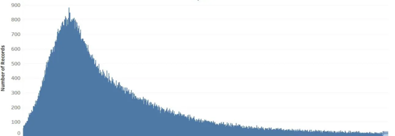
Figure 3.3 Trip Duration
4. Demand Analysis
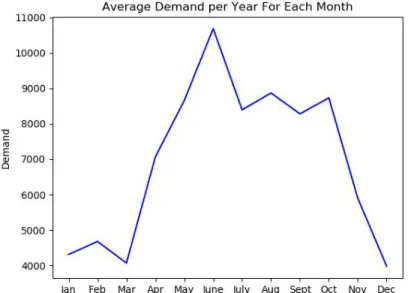
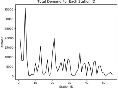
As shown in the figures 4.1 and 4.2 below, the demand among different bike stations vary a lot and the average demand vary a lot in different month. In this section, what I am trying to do is to build a prediction model to prediction the daily demand of a certain bike station.
Figure 4.2 Total demand for each station
4.1 Methods
In order to build the prediction model and analysis the influence of weather on the bike demand, two different sets of features are compared in this section. Feature set (a) include the basic date information without the weather data, while the other feature set (b)
include both the date information and the weather in formation. Both of the features selected for the models are shown below.
Feature set (a): ifweekday, dayofweek(from 0 to 6), weekoftheyear(from 1 to 54)
Feature set (b):ifweekday, dayofweek(from 0 to 6), weekoftheyear(from 1 to 54), WSF5 (miles per hour ), Tavg ( Fahrenheit ), SNWD ( in inches)
weekoftheyear. Ifweekday presents if the trip happened on week day, if so, this parameter equals 1, otherwise, equals 0. Similarly, the dayofweek and weekoftheyear shows the number of day of the trip start date within that week and the number of week within that year respectively.
Feature set (b) contains feature set (a) and three more weather features, the WSF5, Tavg and SNWD. WSF5 is the fastest 5-second wind speed, Tavg is the average
temperature of the day and SNWD is the snow(rain) depth. Those three parameters present the wind, temperature and snow(rain) of the trip day quantitatively.
4.1.1 Lasso Regulation used on Generalized Regression Model
To build the model for demand prediction, I decided upon implementing a linear Regression technique. The reason for this choice was that we can choose a target
The LASSO (Least Absolute Shrinkage and Selection Operator) is a regression method that involves penalizing the absolute size of the regression coefficients. By penalizing (or equivalently constraining the sum of the absolute values of the estimates) we end up in a situation where some of the parameter estimates may be exactly zero. The larger the penalty applied, the further estimates are shrunk towards zero.
4.1.2 K-means Clustering Method
I also employed K-means clustering to cluster pairs of stations based on the demand between them. To build these models we first extracted three features for each pair of stations. For every station pair I have the weekday (1 if weekday, 0 otherwise),
week-number(1-52) as the first two features and daily demand, which is the number of daily trips between these two stations as the third feature for the clustering.
Clustering is an unsupervised learning problem whereby we aim to group subsets of entities with one another based on some notion of similarity. The algorithm is as follows:
1. Choose a center uniformly randomly from the data points
2. Calculate distance between each data point and the center nearest to it and call it D(x)
3. Choose a new data point randomly as center, with weighted probability distribution proportionate to D(x)2 for an element x
This seeding method greatly improves the final error rates of K-means.
4.2 Experimental Results
4.2.1 Generalized Linear Regression
With Lasso model selection to build the model, I also use four fold cross validation for model evaluation. By comparing two different sets of predictors, we surprisingly find that week number ,weekday and if weekend , these three parameters yield a strong
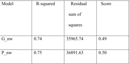
performance. The result of two different models using two sets of features are compared in Table. Four different models are generalized linear model using Gaussian distribution to predict demand without weather features (G_nw) , generalized linear model using Poisson Distribution without weather features (P_nw), generalized linear model using Gaussian distribution to predict demand with weather features (G_w) and generalized linear model using Poisson distribution to predict demand with weather features (P_w).
Table 4.3 Performance of four different models
Model R-squared Residual
sum of squares
Score
G_nw 0.74 35965.74 0.49
G_w 0.86 29379.44 0.73
P_w 0.89 26453.98 0.76
The score in the table 4.3 is the coefficient of determination R^2 of the prediction. The coefficient R^2 is defined as (1 u/v), where u is the residual sum of squares ((y_true -y_pred) ** 2).sum() and v is the total sum of squares ((y_true - y_true.mean()) ** 2).sum(). The best possible score is 1.0 and it can be negative (because the model can be arbitrarily worse). A constant model that always predicts the expected value of y,
disregarding the input features, would get a R^2 score of 0.0.
We can see from the table 4.3 that R-squared measures how this model fit the training data,the models without weather features have explained most of the demand predict.
Despite the season and the weather, demand of bikes can be predicted well with only the date number. At the same time, weather factor helps a lot as well in demand prediction. When weather features are added in the model, the score of model increase from 0.49 to 0.73. While using two different distributions in the model didn’t give much difference in the result. The Poisson model performs slightly better than the Gaussian model.
Figure 4.4 Demand Prediction without weather factors
Figure 4.5 Demand prediction with weather elements
and wider variance based on other factors and the demand of bike in a year is a curve line rather than a straight line. The Figure b that include the weather features in the model resolve those problems and gives a reliable prediction result. We can see that weather factor has great influence on the result. All three weather elements in the model (temperature, wind and rain/snow) contributes to the result a lot.
4.2.2 Clustering Model
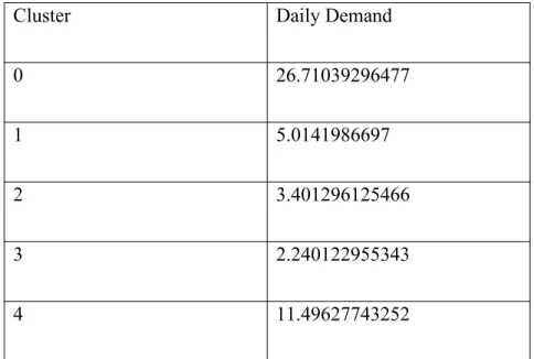
I use K means clustering method to cluster station pairs and their daily demand. I select each station as the begin point and another station as the end point. Then I calculate the demand for that specific bike trip route. The best error rate with K- means comes with the parameters k=5, maxiterations=10 and runs=10. Table shows that here are 5 clusters with different average daily demand between the pairs of stations that fall in each of these clusters respectively. Cluster 0 consists of pairs of stations that have high demand between them while Cluster 3 can be thought of as the cluster that has pair of stations with low daily demand.
On exploring these clusters further, we can find that one of the highest demand is between the Yankee Ferry Station in the Governor’s Island and itself. This could be
long and would have taken 40 minutes on average to complete. So the clustering model gives a reasonable result.
Table 4.6 Clustering Result
Cluster Daily Demand
0 26.71039296477
1 5.0141986697
2 3.401296125466
3 2.240122955343
5. Gender Prediction
As we can see from earlier analysis, Of subscriber-based rides in January through December 2017, men took 72.3% of all trips, and women 27.7%. In this section ,I want to discuss what is the cause of this disparity, and how can it be resolved? Can we design a model to predict the gender of the user when the user information is missing?
Figure 5.1 Top Ten Citi Bike Stations with the most male users and Top Ten Citi Bike Stations
with the most female users
(b)
Figure 5.2 Trip Duration Distribution within two gender group , (a) male group ,(b) female
group
Also, after visualizing the trip duration for two different gender groups, we surprisingly find that despite the similar distribution of trip duration between those two groups, the median number for the female group is actually bigger than the male, which indicates that female tend to use Citi Bike for longer time. As for the male group, most of the trips they made are less than 350 minutes. It is a reasonable time period for commuters and light exercise. While we are surprising to find that within the female group, around 40 percent of the trips are longer than 350 minutes. This may indicate that the trip duration can be used to analysis the different usage pattern between two different gender groups.
Given those characteristics, we assume that the duration and the start station location can be useful to predict the user gender.
5.1 Method
in the Citi Bike trip data set) to conclusions about the item's target value (gender of the rider ). One of a great advantages of decision analysis is that a decision tree can be used to visually and explicitly represent decisions and decision making. For this analysis, it is easily for us to understand how this model is built.
5.2 Experimental Result
Among total 273886 trips in 2017, 72.3% of the records were contributed by the male rider. So in this model the base line for the model performance is 72.3%
Like the demand analysis model, I use the four-fold cross validation to measure model performance. After training the model , the accuracy is 83.2%. The decision tree figure is as shown below.
Figure 5.3 Decision Tree Model
start point and end point and the date (the number of the date within a week) is informative for gender prediction.
Figure 5.4 Decision Tree Model (Part)
What is worth noticing is that there is a usage pattern stand out for female users who are older than 70 years old and live inside New Jersey (As shown in Figure 5.4) Recall that gender 1 represent male and gender 2 represent female. The first two boxes are mainly female based on the value. Even though this user group is not large, they share a unique usage pattern. This also match our earlier observation that the elder group stands out in gender analysis. Different from other age groups, female users are way more active than make users among users over 70 years old. And this user group has a specific
preference on the start start station, most of which are in quiet residental area.
5.3 Discussion
numbers to safety among car traffic.” Considering Citi Bike’s distribution across some of the most congested parts of Manhattan and Brooklyn, lower female participation makes sense. Further analysis of the gender divide by bike share station shows that bike stations in North New Jersey and Manhatten are predominantly used by men, while South New Jersey stations are more proportionately popular among women. Of the top ten stations for each gender, women preferred the New Jersey residential neighborhoods. Also, the same study shows that women also chose stations in areas with fewer lanes of traffic, more limited truck traffic, fewer collision-based cyclist injuries in recent memory, and in some cases, fast access to bridge entrances; men most often chose stations with more traffic, some truck traffic, some collision-based cyclist injuries, and, typically,
6. Comparison between the usage of Citi Bike and NYC Cab
Since the cab data set’s size is 100 times bigger than the bike trip data set, to get a better visual result, I used random sample method to create a sub cab data set that match the size of the bike data. To see the distribution of the pick up points of two samples, I take a random sample from the taxi data set of 3000000 records, which shares the same
Figure 6.1 Pick up Points of Bike Trips and Cab Trips
6.1 Data Cleaning and Feature Extraction
The speed is calculated separately in two different methods. The cab speed is easy to calculate simply use the distance and trip duration (trip end time minus trip star point). However, the trip distance is not provided in the Citi Bike data set. In this case, I assigned a new feature called L1 distance to each Citi Bike trip data. Different from using the direct distance between the start point coordinate and the end point coordinate, L1
distance provide a closer estimate to the real distance having in mind the grid structure of Manhattan (and beyond).
I define a new array w ([0.874804, 0.484478]) as the unit vector along the Avenue direction , pointing towards NNE. And the L1 distance, instead of returning the distance of the hypotenuse between the start point and the end point, gives the sum of the
distances of two legs of the right triangle whose leg indicates the vector w.
6.2 Comparison on Average Speed
(a) Taxi (b) Citi Bike
The Figure 6.2 shows that the distribution of the average speed show great difference, the cab clearly has a wider distribution in terms of speed, while most of the bike trips’ speed remain in a relative low level. This finding is quite intuitive. While, the distribution of the distance between those two method is surprisingly similar. The median value of the trip distance of the cab sample is just slightly larger than the bike.
Figure 6.3 Relationship between Speed and Distance
From the figure 6.3 above, it is clear that there is a large overlap between the two data sets in terms of the trip distance and trip velocity. So, it is not necessary that cab is always faster than the bike in New York City.
Figure 6.4 Speed Comparison
6.3 Comparison on Usage pattern
We stack all weeks in the data set and compute the number of bikes and taxi trips that start within one hour window (normalized to the total number for sake of visualization).
Figure 6.4 shows an interesting pattern of the usage of bike. The peaks of bike usage in weekdays are during morning and evening rush hours, which indicate that many bike users choose to use Citi Bike for daily commute. While the usage pattern in weekends show great difference from the usage in weekdays. The only peak in weekends appear around moon, which maybe because that people tend to use Citi Bike as a leisure and prefer to go out during the warm hours. The usage pattern of taxi didn’t show large difference between weekdays and weekends. The evening usage peak of the usage of bikes appear eariler than the taxi’s evening peak. This may be because of the sunset will influence the willing of people to use bikes as their transportation method. Also, the taxi demand shows that their are two peaks in the evening rush hour, appear around 7 and 11 separately. This pattern is especially obvious on Fridays and Saturdays. This may indicate that taxi is still the main transportation choice for after-hour leisure activities compared to bikes. And as the demand of taxi reaches peak on Friday nights and Saturday nights, the demand for Citibikes drops correspondingly. This is also a evidence that shows that Citibike is a replacement for taxi for many people.
7. Discussion
Based on the experiments and explores discussed above, we can see that the hypotheses I brought up in the beginning part is basically verified. The usage of Citi Bike system follows a pattern that influenced by the weekday/weekend and the weather a lot. The difference of the demand and speed of the bike is clear between weekdays and weekends. Based on the different usage pattern, a predict model using generalized linear regression algorithm can be used to predict the daily demand on the Citi bikes of a certain bike station. The model combines weather factor and date information, and gives satisfying result. Also, two different gender group have its unique usage habit. Even though men took most of the usage of the Citi bike trips, women tend to take a longer trip than wen based on the trip data. In order to encourage more women to join the biker family, creating a new bike-friendly environment may be helpful. As for the elder group, female shows active usage pattern compare to male. So to the bike sharing company, it may be nice to take more care of the elder female group since they are already a steady user group of the bike sharing service. Since the limitation on the data source, this study studies only involve weather factors. For further study on the usage pattern and demand analysis, social factors can be also studied like major social event etc. Also, users can be categorized with more details like students, travelers and commuters etc.
that the bike sharing systems can not only provide people a convenient way for physical exercise but also release the pressure on urban traffic and air pollution. Given that fact that the demand for taxi do decrease when people are using Citi bikes, it is reasonable to encourage people to use bike sharing services for short commute instead of using taxis or private vehicles. The study on the average speed gives similar conclusion. It turns out that during the peak hours, Citi bikes can be a even faster choice. It is easy to
understand that people prefer a warmer and safer choice, like taxi, at Friday or Saturday night after hanging out with friends. But during the daytime especially in spring or summer, bikes can be more efficient than taxis. Also, more studies can be done using this public bike sharing data. For further study, more elements and predictors can be included in the prediction model like the household income among different areas in New York City to enhance the performance of the model. Also, comparison on the bike
8.Conclusion
This project is data analysis project and the best lesson I learned is to comprehend the data as thoroughly as possible. Before conducting the real experiment, research on the similar studies and practices are needed. Those preparation can helps with creating a clear framework of the experiments and having a specific assumption in mind. In this project, the data collection, data cleaning and the feature extraction takes most of the time, which I believe is true to most of the data analysis projects. Only after those preparation can you make sure that this project is feasible and meaningful. The data pre-processing procedure is full of unexpected errors and cause a lot of problem to me. The problems include unavailable data, messy data, disordered data schema etc. What I learned in SILS help with managing the project in a productive way and foreseeing the possible problems. Even thought the preparation took longer time than expected, the result is not influenced by this problem.
Also, in this project, different types of data models are used. The correct understanding of the model is built on the understanding of the data. This project contains knowledge from not only information science but also statistics and urban planning. Those domain
Bibliography
Jon Froehlich, Joachim Neumann, and Nuria Oliver. Sensing and Predicting the Pulse of the City through Shared Bicycling. In IJCAI, 2009
P. Borgnat, C. Robardet, P. Abry, P. Flandrin, J. Rouquier, and N. Tremblay. A Dynamical Network View of Lyon’s Vélo’v Shared Bicycle System. In Dynamics On and Of Complex Networks, volume 2, chapter A Dynamical, pages 267–284. Springer Berlin Heidelberg, 2013.
Faghih-imani, A., Eluru, N., El-geneidy, A. M., Rabbat, M., & Haq, U. (2014). How land-use and urban form impact bicycle flows : evidence from the bicycle-sharing system ( BIXI ) in Montreal. Journal of Transport Geography, 41(August 2012), 306–314. https://doi.org/10.1016/j.jtrangeo.2014.01.013
Mátrai, T., & Tóth, J. (2016). Comparative Assessment of Public Bike Sharing Systems. Transportation Research Procedia, 14, 2344–2351.
Volume, M. E., Me, I., & Meng, O. (2011). Implementing bike-sharing systems, 164. https://doi.org/10.1680/muen.2011.164.2.89
(*)Zhang, Y., Thomas, T., Brussel, M. J. G., & Maarseveen, M. F. A. M. Van. (2016). Expanding Bicycle-Sharing Systems : Lessons Learnt from an Analysis of Usage, 1–26. https://doi.org/10.1371/journal.pone.0168604
Zhang, L., Zhang, J., Duan, Z., & Bryde, D. (2015). Sustainable bike-sharing systems : characteristics and commonalities across cases in urban China. Journal of Cleaner Production, 97, 124–133. https://doi.org/10.1016/j.jclepro.2014.04.006
O’Brien O, Cheshire J, Batty M. Mining bicycle sharing data for generating insights into sustainable transport systems. Journal of Transport Geography. 2014; 34:262–73.
. Fuller D, Sahlqvist S, Cummins S, Ogilvie D. The impact of public transportation strikes on use of a bicy- cle share program in London: Interrupted time series design. Prev Med. 2012; 54(1):74–6. doi: 10.1016/ j.ypmed.2011.09.021 PMID: 22024219
Kaltenbrunner A, Meza R, Grivolla J, Codina J, Banchs R. Urban cycles and mobility patterns: Exploring and predicting trends in a bicycle-based public transport system. Pervasive and Mobile Computing. 2010; 6(4):455–66.
Vogel P, Greiser T, Mattfeld DC. Understanding Bike-Sharing Systems using Data Mining: Exploring Activity Patterns. Procedia—Social and Behavioral Sciences. 2011; 20:514–23.
Beecham R, Wood J. Exploring gendered cycling behaviours within a large-scale behavioural data-set. Transportation Planning and Technology. 2014; 37(1):83–97.
Zhao J, Wang J, Deng W. Exploring bikesharing travel time and trip chain by gender and day of the week. Transportation Research Part C: Emerging Technologies. 2015; 58, Part B:251–64.
Zhou X. Understanding Spatiotemporal Patterns of Biking Behavior by Analyzing Massive Bike Sharing Data in Chicago. PLoS ONE. 2015; 10(10):e0137922. doi: 10.1371/journal.pone.0137922 PMID: 26445357
Jappinen S, Toivonen T, Salonen M. Modelling the potential effect of shared bicycles on public transport travel times in Greater Helsinki: An open data approach. Applied
Jensen P, Rouquier J-B, Ovtracht N, Robardet C. Characterizing the speed and paths of shared bicycle use in Lyon. Transportation Research Part D: Transport and Environment. 2010; 15(8):522–4.
Goodman A, Cheshire J. Inequalities in the London bicycle sharing system revisited: impacts of extend- ing the scheme to poorer areas but then doubling prices. Journal of Transport Geography. 2014; 41.
Lathia N, Ahmed S, Capra L. Measuring the impact of opening the London shared bicycle scheme to casual users. Transportation Research Part C: Emerging Technologies. 2012; 22:88–102.
Appendix
1. Citi Bike Trip Histories data schema
Citi Bike Company publish downloadable files of Citi Bike trip data. The data includes:
Trip Duration (seconds) Start Time and Date Stop Time and Date Start Station Name End Station Name Station ID
Station Lat/Long Bike ID
User Type (Customer = 24-hour pass or 3-day pass user; Subscriber = Annual Member)
Gender (Zero=unknown; 1=male; 2=female) Year of Birth