ABSTRACT
R.M. Pratt: A Vehicular Portal Monitor
A Nal monitoring system was assembled and installed to provide radiological surveillance of refuse trucks
destined for the sanitary landfill at Brookhaven National Laboratory. The performance of the system was tested by obtaining count rates for various gamma reference sources placed in the bed of a pickup truck parked over the
detector. The system's sensitivity was documented for the various sources counted in a stationary truck as well as in a truck moving over the detector. Data analysis also determined the lower limits of detection for the system.
Performance testing of the vehicular portal monitor suggest that it can detect uCi amounts of radionuclides on
Those to whom I am indebted are many. First and
foremost, I offer my gratitude to Dr. James Watson for his extraordinary abilities as an educator. His support and
guidance made possible my most valuable learning
experience.
I also express my appreciation to Dr. Joseph Shonka of
Brookhaven National Laboratory without whose knowledge, strength and advice this project would not have taken root. I would like to thank the staff of Brookhaven's Safety and Environmental Protection Division, namely
Messrs. Joseph Balsamo, Joseph Klemish, George Hughes and
Mien Jones for their cheerful assistance.
Finally, ray heartfelt thanks go to my parents for their love, patience and endless generosity.
Page
Chapter I. Introduction
Obj ective... 1
Scope... 2
Other Vehicular Portal Monitors... 3
Chaper II. Equipment and Installation Electronics ... 5
Other Equipment... 6
Assembly of Detector Head ... 8
Placement of Equipment at Test Site... 9
Check Sources... H Monitoring Modality of System... 14
Background Survey of Test site... ig Chapter III. Testing Procedures Selection of Detector Size: Signal-to-Noise Ratio... 19
Determination of Solid Angle of Detection . . 20 Determination of Dead Time... 24
Determination of Linearity... 25
Determination of On-Vehicle Sensitivity 28 Stationary-Vehicle Sensitivity... 30
Amersham Sources... 32
Brookhaven Sources... 36
Moving-Vehicle Sensitivity... 39
Determination of Lower Limits of Detection . 40
Chapter IV. Results Signal-to-Noise Ratio ... 45
Solid Angle of Detection... 46
Dead Time... 48
Linearity... 49
Sensitivity... 52
Stationary-Vehicle Sensitivity... 52
Amersham Sources... 52
Brookhaven Sources... 55
Moving-Vehicle Sensitivity... 62
Chapter V. Discussion
Sensitivity Curves for Amersham Sources ... 70 Sensitivity Curves for Brookhaven Sources . . 72 Comparison of Sensitivity Findings... 73
Lower Limits of Detection Curves ... 83
Chapter VI. Conclusion and Recommendations 89 APPENDIX I. Method for Determining Sensitivity . 93 APPENDIX II. Method for Determining Dead Time
Corrected Sensitivity ... 103 APPENDIX III. Method for Determining Lower
Limits of Detection... 105
Bibliography... 109
Page
1. System Schematic...7
2. Detector Head Assembly...2.0 3. Electronics Housing ... 12
4. VPM Test Site...13
5. Background Survey of Test Site...18
6. Solid Angle Geometry...22
7. Variation of Observed Rate (m) as a Function of True Rate (n)...26
8. On-Vehicle Source Alignment at VPM Test site. . 31 9. Dimensions of Solid Angle Geometry...47
10. Linearity of Detector...51
11. On-Vehicle Sensitivity Curves, Amersham Sources on Stationary Vehicle...71
12. Sensitivity Curves for Stationary and Moving Vehicle, Brookhaven Sources...74
13. Comparison of Stationary-Vehicle Sensitivity, Amersham and Brookhaven Sources...75
14. Comparison of Stationary-Vehicle Sensitivity, Amersham and Brookhaven Sources (Dead Time Corrected Values)...78
15. Comparison of Sensitivity for Brookhaven Sources (Dead Time Corrected Values) on Stationary and Moving Vehicle...81
16. LLD Curves for Amersham Sources on Stationary Vehicle...85
Vehicle...87
Page
1. Amersham Reference Sources ... 33
2. Brookhaven Reference Sources... 37
3. Signal-to-Noise Ratio... 45
4. Linearity Test Results... 50
5. On-Vehicle Gross Counts/30 Seconds, Amersham Sources... 53
6. On-Vehicle Net Counts/30 Seconds, Amersham Sources... 54
7. On-Vehicle Net Counts/Minute, Amersham Sources 56 —5 8. On-Vehicle Sensitivity (10 Counts/Gamma) vs. Photon Energy, Amersham Sources... 5 7 9. Stationary-Vehicle Gross Counts/30 Seconds, Brookhaven Sources... 5 8 10. Stationary-Vehicle Net Counts/30 Seconds, Brookhaven Sources ... 59
11. Stationary-Vehicle Net Counts/Minute, Brookhaven Sources ... 59
-5 12. Stationary-Vehicle Sensitivity (10 Counts/Gamma) vs. Photon Energy, Brookhaven Sources... 61
13. Dead Time Corrected Net Count Rates (cps) for Brookhaven Sources on Stationary Vehicle . . 62
-5 14. Dead Time Corrected Sensitivity (10
Counts/Gamma) for Brookhaven Sources on
Stationary Vehicle... 6 3
16. Moving-Vehicle Net Counts/4 Seconds,
Brookhaven Sources... 64
17. Moving-Vehicle Net Counts/Second, Brookhaven
Sources... 65
—5
18. Moving-Vehicle Sensitivity (10 Counts/Gamma)
vs. Photon Energy, Brookhaven Sources. ... 66 -5
19. Dead Time Corrected Sensitivity (10
Counts/Gamma) for Brookhaven Sources on Moving
Vehicle... 66
20. Lower Limits of Detection (yCi) on Stationary Vehicle, Amersham Sources... 67
21. Lower Limits of Detection (UCi) on Stationary
Vehicle, Brookhaven Sources (Dead Time
Corrected Values)... 68
22. Lower Limitsof Detection (uCi) on Moving Vehicle, Brookhaven Sources (Dead Time
Corrected Values)... 69
Objective
The purpose of this project was to design, assemble and test a prototype vehicular monitoring system to detect inadvertent radioactivity on refuse trucks destined for the sanitary landfill at Brookhaven National Laboratory
(BNL). Located in Upton, L.I., N.Y., BNL has operated as a research facility devoted to peaceful uses of atomic energy since 1947. Radioactive waste generated at the laboratory is handled on-site at the Hazardous Waste
Management Facility. The sanitary landfill at Brookhaven is designated to receive all non-toxic waste generated by
the various research facilities.
Routine radiological surveys at BNL have indicated the presence of small quantities of activated or contaminated waste in the landfill. For this reason the Safety and Environmental Protection Division (SEPD) of BNL has
committed itself to initiate radiological surveillance of
refuse traffic destined for the landfill.
To this end, a vehicular portal monitor (VPM) was assembled and tested. The procedures and results of this
will be collected and analyzed periodically by the SEPD
staff. The number of trucks carrying refuse to the
landfill and the proportion of contaminated traffic will be determined. These results will be a decision factor for the installation of a permanent vehicular portal
monitor at the landfill.
Scope
The scope of the project was to assemble, install and test the prototype VPM using a Nal crystal as a means of
detection. The Nal detector head was assembled and buried
at a test site at the side of the primary access road leading to the landfill. The associated electronics of
the system were installed at the site and protected from
environmental conditions by a custom-made wooden housing.
The system was powered by a 110 volt power supply. An aluminum plate was placed over the face of the detector
head to protect it from the passage of vehicles.
The system was automated to document the passage of a vehicle and record the level of radioactivity detected
during a counting interval activated by a pressure tube
tripping device. Radiation levels on a truck were
determined by recording count rates with a counter/timer
and a strip chart recorder. The system was also designed
to record background radiation in hourly counts
determination of detection sensitivity for various
nuclides counted on a stationary truck parked over the detector. Sensitivity for nuclides counted on a truck moving at 5 mph over the detector was also considered in
this study. Further analysis of the counting data determined lower limits of detection (LLD) for each nuclide on both a stationary and moving vehicle.
Qthgr yghjcul^r Port^i Monitors
A computer search of nationwide literature performed
at the BNL library yielded no information on vehicular
portal monitors employing a Nal crystal as a means of detection. One commercially available system designed to monitor vehicles was found. It was manufactured by the
IRT Corporation of San Diego, California and operated on the principle of liquid scintillation detection (Ba 84) .
The only vehicular portal monitor based on Nal
detection was one custom-designed by the Health Physics
personnel at Los Alamos National Laboratory (LANL) in New
Mexico. This detector had gained some fame by detecting a truckload of contaminated metal which originated at the
Jonke Fenix scrap metal yard in Juarez, Mexico. It was
this device that triggered an investigation leading to the
discovery of the Juarez incident where recycled metal was
crystal located beneath an aluminum manhold cover in the
road at the gate of an accelerator facility. The system made use of two Nal crystals, one above ground and one
below ground, to correlate on-vehicle radiation levels
with background variability. The LANL system operated on
a tripping system which activated the electronics to record data. The system was also designed to photograph any vehicle that triggered a radiation alarm. The written report on the LANL vehicular portal monitor had not been completed and, because of LANL's defense contract, further details concerning this portal monitor were unavailable
Materials used for fabrication of the VPM and
procedures for installation at the test site are discussed in the following sections. All equipment was provided by the Health Physics Instrumentation Shop at BNL. Workbench
space was made available in the Calibration Shop for assembly and preliminary testing of the system.
Electronics
A list of the electronic components used in development of the system is given below:
NIM bin
High Voltage Supply, Bertan Model NIM 313 Amp/Preamp, Canberra 814
Amp/TSCA, Canberra Model 2015 A (single channel
analyzer)
Counter/Timer, Canberra Model 1776
Serial Scanner/Printer, Canberra Model 2 089 LIN/LOG Ratemeter, Canberra Model 1481L Strip Chart Recorder, Esterline Angus
3X3 inch Nal crystal/photomultiplier tube, Harshaw
A schematic of the final assembly of the VPM is given
in Figure 1.
Other Equipment
The detector head was assembled in the Calibration
Shop. The materials used for fabrication of this unit are
listed below:
Baird well-counter lead pig
Large bottomless steel trash container
Insulating foam
Silica gel Plastic bags
50 foot cables
2
1 inch thick aluminum plate, 2.5 ft .
The Baird well-counter lead pig used in the assembly
of the detector head had been designed to meet the
specifications of a 3 X 3 inch Nal crystal/photomultiplier tube (PMT). The bottom of the well was fitted with the necessary circuitry for electrical connection of the
crystal/PMT unit. Externally, the base of the pig was
equipped with connectors for high voltage (HV) and signal
cables.
The Baird pig provided several inches of lead around
the sides of the Nal crystal to shield it from background radiation and to protect it from environmental conditions
tt
HV
U
AMP/TSCA
RATE METER COUNTER/TIMER
STRIP CHART
RECORDER
SCANNER/PRINTER
To assemble the detector head, the 3X3 inch Nal
crystal/PMT was permanently encased in the steel trash
container in the following manner:
The crystal/PMT unit was fitted into the well of the lead pig to make electrical connection at the base of the well. The HV and signal cables were connected externally
at the base of the pig. This entire unit was enveloped in
several layers of plastic and silica gel was placed inside the plastic to prevent any moisture from coming into
contact with the cable connections.
The pig was then inverted on the floor of the shop and propped up on three bolts to suspend the unit one inch
from the floor. The large bottomless trash can was placed on the floor over the pig and centered around it. The
power cables, connected at the base of the pig, were
positioned along the inside of the can and out over the
rim.
The ingredients of an insulating foam were mixed and
the solution was poured into the trash can, over and
around the lead pig. when it set, the foam rose to surround the pig completely and hardened to fix the detector in place at one end of the steel can. To
complete the assembly, the detector face was capped with a
thin sheet of aluminum, the edges of which were bent over
from environmental conditions, to be buried at the test
site. A diagram of the assembled detector head is given
in Figure 2.
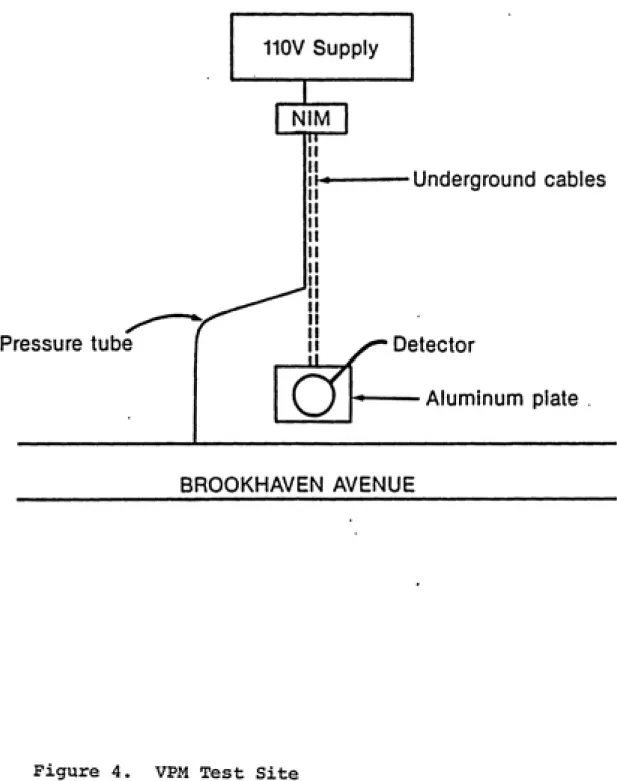
Placement of Equipment at Test site
The test site for the VPM was chosen on the basis of
its proximity to the landfill and the availability of a
110 Volt power supply. The site was located next to
Building 530 at the corner of Brookhaven Avenue and
Seventh Street at the laboratory. The distance between
the landfill and the VPM was about a half mile.The detector head was buried in the ground at the
north side of Brookhaven Avenue. The face of the detector
was situated in the same plane with the surface of the
earth and remained uncovered by soil, A one inch thick,
2
2.5 ft aluminum plate was placed over the face of the
detector to provide protection from the passage of
vehicles.
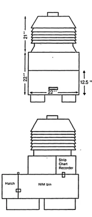
The NIM bin electronics unit was placed adjacent to
the 110 Volt outlet which supplied power to it, A
custom-made wooden housing, built by the HP Instrumentation
staff, protected the electronics from environmental
conditions. This unit was supported by four cement blocks
and incorporated a vented cupola for cooling by natural
Foam. I
Steel can
Al sheet
electronic components. A separate compartment for the
strip chart recorder was located on top of the NIM bin
compartment under the cupola. Figure 3 gives a diagram of
the electronics housing.
The HV and signal cables connecting the detector head
to the associated electronics were recessed below ground
in a 50 foot trench for protection from lawn mowers.
A pressure tube tripping device, similar to those
found at service stations, was fixed above ground about 7
feet in front of the detector head. The pressure tube was
connected to the electronics through the underground
trench. This device was designed to activate the
electronics when tripped by the wheels of a vehicle.
Figure 4 gives a diagram of the equipnent in place at the
VPM test site.
ChecK SQurceg
check sources used for testing the performance of the
VPM were gamma reference sources supplied by the
Radiochemical Centre, Amersham, England. The kit
contained nine point source nuclides encased in
rectangular containers measuring 25.4 x 11,0 x 2.0 mm.
Each container housed a 1 mm. active bead between 0.5 mm
I---1
\
12.5 "
^
strip
Chart
Recordet
ͣ
fi-Hatch
CD
NtM bin
Pressure tube
110V Supply
H---Underground cables
Detector
Aluminum plate
BROOKHAVEN AVENUE
Nucl ide "^Ba "7cs
"co
98^ 22Na
=*Hn 203„.
Activity (i Ci)
8 .96 10 .36 10.12 5 .08 10 .30 8 76 4 .00
Hg
Additional sources used for testing were provided by
the HP Instrumentation Shop and the Hot Lab at BNL. These
sources were contained in large lead pigs because of their
relatively high activity. The Brookhaven sources and the
activity of each are listed below.
mi<pliae Activity (mCi)
"2lr 66.0
i"cs 0.6
"co 7.5
Monitoring Modality of System
The staff of the HP Instrumentation Shop equipped the
VPM with the necessary circuitry to operate a monitoring
modality activated by a signal from the pressure tube
radiation by the strip chart recorder as well as by the
counter. This mode of operation is described as follows.
Barring a signal from the circuit, the system prints
out hourly background counts around-the-clock to keep a
reasonable check on background variability. When the
pressure tube is tripped, the signal activates the strip
chart recorder to run for a 10 second monitoring interval.
The strip chart paper advances at a rate of 20 cm per
minute and records the radiation level in counts per
second as measured by the ratemeter.
At the same time, the signal from the pressure tube
sends a pulse to the printer forcing a print-out of the
accumulated background counts from the previous hourly
print-out. The elapsed time since the last print-out is
also recorded in the one second printing interval.
Following the background print-out, the system begins
to count for two successive 4 second counting intervals,
each of which is followed by a one second printing
interval. During each printing interval the system ceases
to count for one second.
The steps of the monitoring modality are given as
follows:
1. Background print-out (1 sec) plus strip chart
recorder begins 10 second monitoring interval.
2. First counting interval (4 sec).
3. Print-out (1 sec).
5. Print-out (1 sec).
6. Return to hourly background counts.
At the end of 10 seconds the system returns to the
hourly cycle of background counting. With the monitoring
mode activated, further tripping of the pressure tube by
the rear wheels is ignored.
Background Survey of Test Site
The detector head was buried about 3 0 feet from Bldg.
53 0 which once functioned as the Hot Machine Shop. The
building remained posted for radioactivity and, therefore,
it was necessary to perform a background survey of the
area.
A survey meter responding in juR/hour, provided by the
Calibration Shop, was used to survey the area around Bldg.
530 and the general vicinity of the VPM test site.
Readings were taken at a height of 2 feet above ground.
The results of this survey were recorded on a map of the
site and showed the area to be within the range of
background variability for the laboratory.
During the survey, a shipment of high level
radioactive waste passed along Brookhaven Avenue destined
for the Hazardous Waste Management Facility. At this
time, the ^R meter responded off-scale to the high level
of radioactivity passing by the VPM test site.
considerable elevation of background radiation at the test
site. Such an elevation would be recorded by the hourly
background counting modality of the VPM and would not
present a problem unless the situation occurred
simultaneously with the monitoring of a landfill refuse
truck.
If, during the monitoring of a truck, a high level
radioactive waste shipment were to pass by the test site, information regarding the presence or absence of low-level
radioactivity in the refuse would be lost. The
probability of such a coincidence, albeit low, would result in a spurious signal for activity in the refuse
truck and yield a false positive reading for determining
the percentage of refuse trucks shipping inadvertent
radioactivity to the landfill.
The overall background radiation for the BNL site ranged from 8 to 20 ]iR/hr. The major portion of the area around the detector showed background levels of 8 to 10
UP/hr with only one point (next to Bldg. 530) showing a level of 20 yR/hr. The map of the test site in Figure 5
shows the values of the survey readings.
SEVENTH STREET
UJ
Z
LU
2
LU
I
o
o tr
m
SpR/hr
BLDG. 530
20HR/hr
10MR/hr
lOfiR/hr
\ \
. ;
/ /
/ / / /
/
/
Chapter III
TESTING PROCEDURES
Selection of Detector Size; Signal-to-Noise Ratio
The preliminary testing and assembly of the VPM was carried out at workbench space provided in the Calibration Shop at the laboratory. With the NIM bin electronics
assembled at the workbench, the size of the Nal crystal to
be used in the final assembly of the system was
determined.
The decision for selection of crystal size was based on the criterion of signal-to-noise ratio which is an index of a crystal's ability to detect a radiation source in the presence of natural background radiation, assuming a sufficient signal size. This ratio was determined by
the number of recorded counts from a reference source
divided by the number of recorded counts from background
radiation.
Three Nal crystals were available for testing. Each crystal was cylindrical in shape and coupled as a unit with a photomultiplier tube (PMT) . The dimensions of each
crystal were as follows:
3. 8 inches in diameter by 8 inches in height (8 X 8)
The procedure for obtaining data for the signal-to-noise ratio on each crystal was carried out as follows: A
203
4 ^Ci check source of Hg was taped to a one inch thick
aluminum block which was placed in contact with the
crystal surface. The purpose of interposing one inch of aluminum between the source and the crystal was to
simulate the field conditions of placing a one inch thick
aluminum plate over the detector.
A series of five 10 second counts was made and
recorded in average counts per second (cps) . With the source removed, a series of five 10 second counts was made
for background radiation. Background counts were also
recorded in average cps. This procedure was followed for
data collection on each of the three Nal crystals. During the counting procedure, each crystal was shielded from background by stacking lead bricks around the sides of the
crystal.
The signal-to-noise test was repeated on the 3x3
inch crystal placed in the Baird well-counter lead pig.
Determination of Solid Angle of Detection
Solid angle of detection is defined as a three
dimensional angle or solid cone, the apex of which is the face of the detector, subtended by the area of a plane
radiation source is detectable by the system. An
isotropic source of radiation anywhere within the solid
angle will elicit a response by the detector. The purpose of determining the solid angle of
detection of the VPM was to estimate the area in the bed of a truck that can be seen by the detector. Because of
differences in placement of activity in a truck load and
variability of paths taken by the passage of the vehicle
over the detector, the solid angle of detection should be
sufficient to detect a source located anywhere in the bed
of a truck.
The method for determining the solid angle of
detection is described as follows. The assembled detector
head unit was oriented horizontally on the floor of the
137
Calibration Shop. A 10 yCi source of Cs was rolled on
a (^olly along a path (P) parallel to the face of the
detector at a distance (d) of 100 cm at right angles to
the face of the detector. A diagram of this geometry is
given in Figure 6.
The diameter of the detection field along path (P) was
determined in the following manner: Beginning the traverse of path (P) , with the source outside the
detection field, the ratemeter needle indicated a reading
of background radiation at about 10 cps. As the source
entered the detection field, a rapid response of the ratemeter needle above background was noted. This point
Path (P)
^
^
a = radius of detection field
d = source to detector distance a right angle
marked by pencil on the floor of the shop to indicate the
boundary of the detection field along path (P) . The
source was rolled further along path (P) with the
ratemeter indicating continued response. When the
ratemeter needle returned to its position for background
this point (Y) was marked on the floor to indicate the opposite boundary of the field. Measurement between
points X and Y determined the diameter of the detection
field at 100 cm from the detector within which the system
will respond to any activity present.
A distance of 100 cm corresponded to 39.3 inches
between the measured detection field and the detector.
With the bed of the test truck at a height of 30 inches
from the buried detector, the measured detection field was
9.3 inches above the bed of the truck. The diameter of
the detection field at this distance gave an indication of
the area over the bed of the truck that can be seen by the
detector.
The method for determining the solid angle of
detection (fi), in steradians, is given by the expression:
fl = 2 IT
1-ys2
fd^ + a'ͣ
-2
(Kn 79)
where
d = source-to-detect or distance at right angle to
face of detector
Determination o£ Dead Time
Dead time of a counting system is the minimum amount
of time which must elapse between two events in order that
they may be recorded as two separate pulses. Any event which occurs within the dead time of the system is lost
from the total counting of true events, therefore, for
precise measuronent account must be made for dead time losses within the system. Dead time losses become greater
with increasing interaction rates, thus affecting the
ability of the system to measure high rates.
The method for determining the dead time (T) of a
nonparalysable system was the Two-Source Method described
in the NCRP Handbook of Radioactivity Measuronents
Procedures (NCRP 78). This method is based on observing
the rates (n,) and (n^) from counting two sources
individually, the combined source count rate (n, j) ^^^ the
background rate (n, ) .
Because the counting losses are non-additive, the
observed rate from the combined sources (n,2) will be less
than the sum of the rates observed for each source counted
individually, (n, + nj) . Dead time can be calculated from
the discrepancy using the following formula:
T = { 1- [1- { A - n. ) q/p^] } p/q (NCRP 78)
where
p = n^n2 - n^^n^2
q = n^n2n^2 + %("l"2 " "^1 ^^12 ' ^2''l2^
Dead time of the VPM was determined at the test site
using 10 pCi of c"s and 10 pCi of Co counted
individually and in combination. Each count was made with the source (s) in direct contact with the protective
aluminum plate over the detector. The source-to-detector
distance was 3 inches.
1*3*7 C f\ TOT
The sequence of counting was Cs, Co and Cs
plus Co which yielded observed rates n, , n2 and n,2
respectively. Each rate was recorded in average cps
determined from a series of five 3 0 second counts.
It should be noted that the determination of dead time at this time was made on the system which incorporated the Amp/Preamp component in the NIM bin electronics. This
component was later replaced by the Amp/TSCA.
Determination of Linearity
Linearity is the ability of a counting system to
measure accurately increasing interaction rates. An ideal
system would show perfect linearity of measurement over a full range of rates. Because dead time losses are an inherent property of all systems, the deviation of the observed rate from the true rate widens as the interaction rate increases. To illustrate, a plot of observed rate
dashed linear curve represents the true count rate that would be observed with an ideal system. With no dead time
losses m = n. Since losses due to dead time increase with
higher interaction rates, the solid, non-linear curve represents the observed rate (m) as a function of true rate (n).
To determine the deviation from linearity of the VPM the following procedure was carried out at the test site
on the original system using the Amp/Preamp. Three check
sources were counted in contact with the aluminum plate which represented a source-to-detector distance of 3
inches. The three Amersham sources used in this procedure
are listed below.
£Q!IEC£ ACTIVITY
ͣ
••^^Cs 10 yCi ^°Co 10 yCi ^^Mn 8 yCi
Observed rates were recorded for each source, counted
individually and in combination, by a series of five 3 0 second counts. The results of counting each individual source and combination of sources were recorded in average cps as was the background count rate.
CQUNTitNG gEQUEUCE 137
Co
S^Mn
^Oco -H ^'m
l^^Cs + 60co
Background
Values of theoretical count rates for each combination
of sources were calculated by the summation of the ob¬
served net rates obtained from the individual counting of each source, assuming negligible dead time losses for single source counting. For example, the theoretical net
rate for the combination of Co + Mn + Cs was deter¬
mined by summing the observed net rates for each of these sources counted singly. This procedure was repeated to
obtain values of theoretical rates for all combinations of
sources.
Determination of On-Vehicle Sensitivity
The sensitivity of a counting system is defined as the
fraction of photon emissions that interacts with the
detector crystal and is counted (NCRP 78). In this sense, the detection sensitivity is synonymous with the absolute efficiency of the system and is expressed as the number of
On-vehicle sensitivity was determined for each photon energy by counting each source in a truck and dividing the observed net count rate by the photon emission rate of the source. The photon emission rate (gamma/minute) was
determined from the activity (yCi) of the source/ a conversion factor for the number of disintegrations per minute (dpm) per yCi and the photon emission probability
per disintegration (gammas/disintegration). This method
is given by the expression
Gammas/min = activity (yCi) X 2.22 x 10 dpm ^ gammas/
liCi disinte¬
gration.
The expression for determining sensitivity is given by
Sensitivity = observed net count rate (cpm)
photon emission rate (gammas/min) = counts/gamma.
An experiment was designed to determine the on-vehicle
sensitivity versus photon energy for the reference sources used. The design included the determination of
sensitivity for each photon energy versus various thicknesses of sand attenuation on the truck.
On-vehicle sensitivity values were determined by counting the Amersham and Brookhaven sources on a
stationary truck. The Brookhaven sources were used to determine sensitivity on the truck moving at 5 mph over the detector. These methods are presented in the
Stationary-Vehicle Sensitivity
The counting of each source in the bed of a stationary
pickup truck was carried out at the VPM test site. The truck was parked over the detector with the rear axle and differential aligned directly over the detector head.
Placement of each source was in line with the detector.
Counting results for this alignment reflect the maximum inherent shielding of the truck since the differential presented the most attenuation material under the bed of
the truck. The distance from the bed of the truck to the
detector was 30 inches. Figure 8 shows the on-vehicle source alignment with the detector at the VPM test site.
Since any activity in a load of refuse may be shielded by other materials in the load, sensitivity for each
source was determined for various additional attenuation conditions. The sources were counted at attenuation
levels of 0, 3, 6, 9 and 12 inches of sand interposed
between each source and the truck bed. A series of five
30 second counts was made for each source at each sand
level in the truck. Background radiation was counted in
the same manner. The Amersham sources were counted at
five sand attenuation levels, while the Brookhaven sources were counted at 0, 6 and 12 inches of sand attenuation.
The sand was contained in a cardboard box the dimensions
of which were 13 x 9 x 13 inches.
12"sand
9 6
3
\
\
24k.
n
m
system's sensitivity for detecting these sources are given
in the following sections.
Amersham Sources
The Amersham sources used for determining on-vehicle
sensitivity are listed in Table 1, which includes the
activity of each nuclide, the photon energy and photon .
emission probability per decay.
The activity of each nuclide was determined by calculating the remaining activity on the date of
sensitivity testing using the original activity and the
reference time listed on the certificate of measurement
which accompanied the gamma reference source kit. The
radioactive decay equation is given by
A = A e"^^
^t ^0 where
A. = activity remaining after a time interval t
A- = activity of nuclide measured at reference time
A = decay constant for particular nuclide
t = elapsed time
e = base of natural logarithm: 2.718
It should be noted that since the several photon
133
energies emitted by Ba do not vary widely, no
distinction was made among them. Hence, the assigned
133
value for the photon energy of Ba was a weighted
Nuclide 133 Ba 137 Cs 54 Mn 60 Co 22 Na 88, Activity (yCi) 8.96 10.36 8.76 10.12 10.30 5.08
Photon Energy (KeV)
345* 662 834 1250* 1274 511 898 1836 Photon Emission Probability
Per Decay (NCRP 78)
0.98 0.85 1.00 2.00 1.00 1.80 0.934 0.993
applied to using a weighted average for the two energies
emitted by Co.
By a series of five 3 0 second counts, each Amersham source was counted in contact with the bed of the empty
truck. The sources were then counted in contact with the
surface of each sand level in the truck. Each sand level
increased the source-to-detector distance (SDD) by
increments of 3 inches. The SDD for each sand level is
given below.
SAND LEVEL SPP 0 inches 30 inches 3 inches 33 inches 6 inches 36 inches 9 inches 39 inches 12 inches 42 inches
The increased SDD made it necessary to determine
distance correction factors to correct the averaged count
rates of the Amersham sources for a uniform SDD. The
rates were corrected to correspond to a source placement
at 12 inches above the bed of the truck (SDD = 42 inches).Distance correction factors were based on the inverse
square law which states that the intensity of radiation varies inversely as the square of the distance from the
H =
d^Vd,^
where
lo = d, =
d^ =
intensity of radiation at d, intensity of radiation at
d-SDD represented by height of truck bed (30
inches) plus incremental distance added by each level of sand
SDD = 42 inches
The distance correction factors were determined by
^ 2/, 2
d2 /d^
and are given as follows
SAND LEVEL 'inches) DISTANCE CORRECTION FACTOR
0
42^30^ = 1.96
3
42^33^ = 1.62
6
42^36^ = 1.36
9
42^39^ = 1.16
12
42^42^ = 1.00
The net count rates were distance corrected to a SDD
corrected net rate = g^oss rate - background
distance factor
The corrected net counts/30 seconds were converted to counts/minute. Sensitivity for the photon energy of each
Amersham source was determined by
... .. corrected net rate (cpm)
Sensitivity = __________________________ ^ ______ photon emission rate (gammas/minute) = counts/gamma
This procedure determined the sensitivity of the VPM
for the Amersham sources which reflected a source
placement of 12 inches above the bed of the truck.
Brookhaven Sources
Stationary-vehicle sensitivity testing was repeated
using the Brookhaven sources. Since these sources were of greater activity than the Amersham sources, they provided
more statistically significant data. The particulars of
the Brookhaven sources are listed in Table 2.
The activity of each Brookhaven source was determined
by measuring the exposure rate in R/hr at one foot (30.48 cm) from each source with a survey meter due to a lack of
documentation of source activity. Determination of
activity from the exposure rate is given by the following
Nuclide Activity (mCi) Photon Energy
Photon
Emission Probability Per Decay_____
192
Ir 66.0 374 KeV* 2.08
137
Cs 0.6 662 KeV
0.85
60
Co 7.5 1250 KeV* 2.00
* weighted average of photon energies
Q = A^
r
where
Q = activity (mCi)
X = exposure rate (R/hr)
d = source-to-detector distance (cm)
2
r = gamma ray constant (R cm /hr mCi) for the
particular nuclide
Procedures for counting these sources on a stationary
truck were similar to those previously described for the
Amersham sources. The source and truck alignment remained
the same. A series of five 30 second counts was recorded
for each source. Sand levels of 0, 6 and 12 inches were
interposed between each source and the bed of the truck.
This time the position of each source was fixed at 12
inches above the bed of the truck to provide a uniform SDD
of 42 inches.
The NIM bin electronics had been modified by the SEPD
staff during the time between counting the Amersham sources and counting the Brookhaven sources. The
Amp/Preamp used initially in the system had been replaced
by the Amp/TSA. The effect of this change on the counting
data will be discussed later.
Determination of sensitivity for gamma energies
emitted by the Brookhaven sources was made using similar
eliminated the need to distance correct the data.
Moving-Vehicle Sensitivity
An experiment was carried out to determine sensitivity
by counting the Brookhaven sources in the pickup truck moving at 5 mph over the detector. Moving-vehicle
counting data were recorded by driving the truck over the detector and tripping the pressure tube which activated
the monitoring modality of the VPM.
The positioning of each source and the sand
attenuation levels were the same as described previously, i.e. each source was taped at 12 inches above the bed of the truck and 0, 6 and 12 inches of sand were interposed
between the source and the truck bed. with each source in
place, the truck was driven at a speed of 5 mph over the
detector. A series of five runs was made in this manner
for each source at the various attenuation levels.
Background data were recorded in the same manner.
The monitoring modality of the system recorded two 4
second counts for each run. The sources were actually
seen by the detector only during the first 4 second counting interval since the truck was well beyond the detector by the time of the second 4 second count.
gross count rate to determine the average net counts/4
seconds.
Moving-vehicle sensitivities for photon energies of
these sources were determined by converting each net rate to counts per second and dividing by the photon emission rate in gammas/second. The resulting sensitivity values
for the photon energy of each source on a moving vehicle
were recorded in counts/gamma.
Determination of Lower Limits of Detection
To estimate the amount of a radionuclide that could
escape detection by the VPM it was necessary to determine
the lower limits of detection (LLD) , also referred to as the minumum detectable activity (MDA) for each nuclide.
The net count rates recorded for the Amersham and Brookhaven sources were used for this determination.
LLD has been defined by Pasternack as "the smallest
amount of sample activity that will yield a net count for
which there is a confidence at a predetermined level that activity is present" (Co 80). Determination of the LLD is related to the characteristics of the counting system and
is based on statistical hypothesis testing for the
presence of activity. Since the LLD is derived
statistically, the use of the term does not denote an
absolute level of activity that can or cannot be detected,
minimum level of activity that may be detected with
confidence (NCRP 78) .
Hypothesis testing is a form of decision process
whereby sample data are assembled to produce a value that leads to a choice between two decisions, i.e., accept or
reject the hypothesis (Re 7 0) . In the case of the LLD,
the choice is between accepting a value of net counts as a
true signal for detection of activity, or rejecting this
value as non-detection of activity.
In such a decision process, one can never be absolutely certain that the correct choice was made
because of two types of error inherent in hypothesis testing. Currie describes Type I error as deciding that activity is present when it is not. The probability of
making a Type I, false detection error is given by a.
Type II error is described as failing to decide that
activity is present when it is. The probability of making a Type II, false non-detection error is given by g. Since
the probability for both types of error should be kept low, it is customary to accept a level of tolerance for both a and 3 equal to 0.05 (Co 80) (NCRP 78) (Cu 68).
In any discussion of LLD two terms. Critical Limit
(Lp) and Detection Limit (Lj^), must be defined. L^, is the
number of net counts which must be exceeded to yield a
decision of "detected". It is established a posteriori
from the data at hand by the acceptable value for a
signal when the mean of the net counts equal zero. Such a sample count is analogous to background counts.
Mathematically L-, is given as
^C = ^^o (Cu 68)
where
^n, ~ i^PP®^ percentile of the standardized normal variate corresponding to a = 0.05.
s = standard deviation of the sample when the mean of
the net counts is equal to zero (Standard deviation of background counts) ,
L_^ is the signal level such that the number of net
counts at or above this level is likely to be detected.
It is established a priori by specifying the Lp, the
acceptable probability for false non-detection 3 and the
standard deviation of net counts when the mean of the net
counts equals the L_^. Mathematically, the detection limit
is given as
S = L^, + kgSj^ = k^s^ + kgSj^ (Cu 68)
where
kg = upper percentile of the standardized normal
variate corresponding to 3 = 0.05.
s^ = standard deviation of the signal when the mean of
The L_^ is synonymous with the LLD and is the signal
level such that a signal at or above this level is likely
to be detected with confidence.
Currie has shown that, with equal values of a and 3
such that a = g = 0.05, the expression for the L_ is given
as
Ljj = k^ + 2 yr ksj^ = 2.71 + 4.65 Sj^ (Cu 68)
where
k^ = 1.64: the value of the standardized normal
deviate corresponding to the preselected risk for
a = 0.05.
s, = standard deviation of background counts.
The working expression used for determining the LLD
for the VPM is given by:
LLD = C (2.71 + 4.65 s^) (Co 80)
where
C = proportionality constant relating the detector response to the activity, such as C = 1/e where e
Values of LLD for each nuclide were determined from
the same counting data as were used for sensitivity
Chapter IV
RESULTS
Sq.gnal-tQ-Noj,ge Ratio
Results of signal-to-noise testing for selection of crystal size used in the assembly of the VPM are presented
in Table 3.
Table 3. Signal-to-Noise Ratio
CRYSTAL SIZE SIGNAL TO NQISE RATIO
8x8 inch 15 4x2 53
3x3 59
3 X 3 in pig 421
According to the findings, the 8x8 inch crystal showed the lowest signal-to-noise ratio. This relatively low result was due to the fact that the large dimensions of this crystal increased the level of noise faster than
that of the signal. In addition, the dimensions of the 8
The higher values of signal-to-noise ratio for the 4 x 2 inch and the 3x3 inch crystals demonstrated their
greater effectiveness in detecting a radiation source in the presence of background. Results of testing the
smaller crystals showed their signal-to-noise performance
to be comparable. The ratio for the 3x3 inch crystal, however, was greatly increased when it was tested in the well of the Baird lead pig. The factor contributing to this improvement was the excellent shielding from
background radiation afforded by the several inches of
lead surrounding the sides of the crystal.
The Baird lead pig not only improved the signal-to-noise ratio of the 3x3 inch crystal but also provided excellent protection from environmental conditions
encountered by the detector buried at the test site.
These advantages were the decisive factors for selection
of the 3x3 inch crystal to be used in the final assembly
of the system.
Solid Angle of Detection
Solid angle of detection for the detector head was
determined by measuring the distance between points X and
Y which marked the boundaries of the detection field at a
distance of 100 cm from the face of the detector. The diameter of this field was measured to be 210 cm. A
diagram of the solid angle dimensions is given in Figure
210 cm.
-«----105 cm.
^
The solid angle of detection was determined to be 1.9
steradians by the expression
n = 2iT , _ 100 cm
yiOO cm^ + 105 cm'
=1.9 steradians
(Kn 79)
The distance of 100 cm from the detector, at which
the detection field was measured, corresponded to 39.3
inches. With the height of the truck bed at 3 0 inches above the buried detector, the measured detection field
was 9.3 inches above the bed of the truck. The 210 cm
diameter of the detection field corresponds to 6.8 feet
which was the diameter of the area at 9.3 inches above the
bed of the truck that could be seen by the detector.
Pe^<j Time
Results of the two-source method for dead time
determination are given below.
Average gross count rates observed for the counting of
Cs and Co individually and in combination are
presented below as is the average background count rate.
OBSERVED GROSS
NUCLIDE COUNT RATE (CgS)
ͣ
'•^'^Cs (n^) 7361
^°Co (n^) 16252
ͣ
'•^''cs + ^°Co (n^2) 22794
The dead time of the VPM was determined to be 3.5
microseconds using the previously described formula
T = { 1 - [1 - (A - n, ) q/p^]^} p/q (NCRP 78)
This dead time was determined for the original system
which incorporated the Amp/Preamp in the NIM bin
electronics.
Linearity
Table 4 lists the results of counting procedures for
determining deviation from linearity of the original VPM system. The count rate for each single source as well as
each combination of sources counted is listed with the
corresponding observed gross rate, observed net rate and
the theoretical net rate. Theoretical rates for
combination counts were determined by the summation of the
observed net rates obtained from the single counting of each source within the combination.
Since the observed rates for the combination counts
were less than the determined theoretical rates, the plot
of observed rates versus theoretical rates, given in Figure 10, shows the original system's deviation from
linearity due to dead time losses. The dashed curve for the observed rates demonstrates that the discrepan<Y
Somces
54.Mn
137
Cs
54„n + 137^3 ^ 60^0 Background
Observed
GcQSS.Count Ratg (cpsl
V
7120 7361 16252 22557 22794 14086 28769 10
Observed Net Theoretica]. Net
Count Rate icps). Count Rat? (opsl
7110 7110
7351 7351
16242 16242
22547 23352
- 22784 23593
14076 14461
28759 30703
in o. o
<
1-z
O
o o UJ
> cc UJ w m
o 35
30
25
20
15 10 5
0
---Theoretical
---Observed
ͣ
... I . I I ͣ'ͣͣͣͣ'ͣͣ''' ͣ
-5 10 1-5 20
ͣ
I ͣ ͣ ͣ ͣ '...
25 30 35
THEORETICAL COUNT RATE (lO^cps)
Sensiti,vity
Determination of on-vehicle sensitivity was made by
recording count rates for the Amersham and Brookhaven
sources at various sand attenuation levels on the truck
parked over the detector head. Moving-vehicle sensitivity was determined by recording count rates for the Brookhaven sources on the truck traveling at 5 mph over the detector.
Results of counting procedures for stationary and
moving-vehicle sensitivity are given in the following sections.
Stationary-Vehicle Sensitivity
Amersham Sources
Sensitivity versus photon energy was determined for
each of the Amersham sources counted at five sand
attenuation levels'on the stationary truck. The following
tables present the results of counting procedures and
sensitivity for the Amersham sources.
Table 5 lists the average gross counts/30 seconds
observed for each nuclide counted at each sand attenuation
level on the truck. The background rate was an overall average of background counts for each sand attenuation
level. This was used to determine net rates because
background did not vary widely with incremental increases
in sand attenuation.
Table 6 gives the net count rates per 3 0 seconds,
distance corrected to reflect source placement at 12
NucUdg 133, Ba 137 Cs 54 Mn 22 Na 60 Co 88,, 0" S^nd
459 ± 30
732 ± 30
808 ± 22
1883 ± 66 2043 ± 66
1181 + 16
3" sand 359 ± 22 522 ± 36 631 ± 51 1169 ± 18
1369 + 31
899 ± 25
6' Sand
299 + 15 408 + 21 478 + 23 706 + 36 926 + 25
603 ± 37
9" Sand
297 ± 21
353 ± 21
388 ± 46 540 ± 30 600 ± 41
493 ± 37
12'Sand
326 ± 33 332 ± 31 344 ± 22 464 ± 25 515 ± 27 400 ± 18
Background = 292 (19) counts/30 sec.
Nuclide 133,Ba 137 Cs 54 Mn 22 Na 60 Co 88^ 0" Sand
85 ± 25
224 + 25 263 ± 20 812 ± 49 893 + 49 454 ± 18
3' Sand
41 ± 23
142 ± 32 209 + 43
541 ± 21 665 ± 29
375 + 25
6' Sand
85 ± 24 137 ± 26 304 ± 35
466 + 27 229 + 36
aJL£and
**
53 + 26 83 + 46 213 + 33 266 + 42 173 ± 39
^?.' .^aai
**
40 ± 36 52 + 29 172 ± 31
223 ± 33
108 ± 26 * distance corrected to 12" above bed
count rates were determined by subtracting background from
the gross rates and dividing the remainder by a distance
factor. The expression for this determination is given by
Net rate = gross - background
distance factor
where the distance factor at
0" sand = 1.96
3" sand = 1.62
6" sand = 1.36
9" sand = 1.16
12" sand = 1.00
Table 7 shows the distance corrected net rates in
counts/minute which were determined by doubling the net
counts/30 seconds. These values were used to determine
the sensitivity for photon energies emitted by each of the
nuclides.
Table 8 presents the values of sensitivity versus
photon energies of the Amersham sources used in stationary
vehicle testing of the VPM. Values of sensitivity are
—5
expressed in 10 counts/gamma and were determined by
dividing the net count rate (cpm) by the photon emission
rate (gpm) for each gamma energy emitted (See Appendix
I).
Brookhaven Sources
jjuclide 133,'Ba 137 Cs 54 Mn 22 Na 60 Co 88^ 0' Sand 170 ± 50
448 ± 50
526 + 40
1624 ± 98 1786 ± 98
908 + 36
3" Sand 82 ± 46 284 ± 64 418 ± 86 1082 ± 42 1330 ± 58 750 ± 50
(>ͣ Sj>nd
**
170 + 48
274 ± 52
608 + 70 932 + 54 458 + 72
9" sand
**
106 + 52 166 + 92 426 + 66 532 ± 42 346 + 78
1?" JSSM
**
80 ± 72
104 ± 58
344 ± 62
446 ± 66
216 ± 92
* distance corrected to 12" above bed
Energy tnev) 345 511 662 834 898 1250 1274 1836 0" Sand
0.87 ± 0.26
1.73 ± 0.27 2.30 ± 0.26 2.71 ± 0.21 2.71 ± 0.21 3.98 ± 0.22
3.98 + 0.22 5.57 + 0.38
3' sand 0.42 ± 0.24 0.98 ± 0.13 1.46 ± 0.33 2.15 ± 0.44 2.15 ± 0.44
2.96 ± 0.13
2.96 ± 0.13
4.69 ± 0.61
6" Sand
**
0.32 ± 0.18 0.87 + 0.25 1.41 ± 0.27 1.41 + 0.27 2.08 ± 0.12 2.08 + 0.12 2.77 ± 0.69
9" Sand
**
0.38 + 0.17 0.54 + 0.27
0.86 ± 0.47
0.86 ± 0.47
1.18 ± 0.10 1.18 + 0.10
2.29 ± 0.82
12" S9tid
**
0.28 + 0.17 0.41 + 0 37 0.54 ± 0 30 0.54 ± 0 30 0.99 + 0 15 0.99 ± 0 15 1.42 + 0 87
12 inches of sand attenuation in the truck. The reason
for the repetition was to provide more statistically
significant net count rates for low energy photons at the higher attenuation levels. The higher activities of the Brookhaven sources did yield more meaningful results for
192
all data points. The 66 mCi source of Ir, which emits
an average photon energy of 374 KeV, was used in place of 133
Ba (345 KeV) for low energy sensitivity determination
133
because a mCi source of Ba was not available.
Results of counting the Brookhaven sources on the
stationary truck are given in the following tables. Table 9 lists the average gross counts/30 seconds for each of
the sources counted at three sand attenuation levels with
a fixed source placement at 12 inches above the bed of the
truck (SDD = 42 inches). The background count rate is an
overall average value.
Table 9. Stationary-Vehicle Gross Counts/30 Seconds
Brookhaven Sources
Nuclide 0" sand________6" Sand___ ____X2" Sand
ͣ
"
ͣ
^^Ir 1066641 ± 10450 348880 ± 1853 118444 ± 698
ͣ
^^"^Cs 13145 ± 73 5734 ± 64 2042 ± 40
^°Co 389209 ± 744 233811 ± 1028 120264 ± 419
Table 10 gives the average net counts/30 seconds which
were determined by subtracting background from each gross
count rate.
Table 10. Stationary-Vehicle Net Counts/30 Seconds,
Brookhaven Sources
Nuclide 0" Sand__________6" Sand 12" Sand
ͣ
"
ͣ
^^Ir 1066432 ± 10450 348671 ± 1853 118235 ± 698
ͣ
'
ͣ
^^Cs 12936 ± 74 5525 ± 66 1833 ± 42
^°Co 389000 ± 744 233602 ± 1028 120055 ± 419
Table 11 gives the net rates for each source in
counts/minute. These values were determined by doubling
the net counts/30 seconds.
Table 11. Stationary-Vehicle Net Counts/Minute,
Brookhaven Sources
Nuclide _______0" sand_________6" Sand__________12" S^nd
••
ͣ
^^Ir 2132864 ± 20900 697759 + 3706 236471 ± 1395
ͣ
-5
Sensitivity values (10 counts/gamma) for photon energies emitted by the Brookhaven sources are presented
in Table 12.
Because of the higher emission rates of the Brookhaven
sources and the modification of the system by substituting the Amp/TSCA for the Amp/Preamp, it was necessary to
determine sensitivity for the Brookhaven sources from dead
time corrected count rates. The dominant dead time of the
modified system with the Amp/TSCA was 16 ysec (Bi 85).
Net count rates for the Brookhaven sources were
corrected for the increased dead time by the expression
N = "____. - background
(1 - nT)
where
N = true interaction rate
n = observed rate
T = dead time of 16 visec.
Sensitivity for the higher activity sources was then
determined from the corrected net count rates by the
following method.
„ .^. .^ Corrected net count rate (cps)
Sensitivity =_________________________
photon emission rate (gps)
Dead time corrected net count rates for the Brookhaven
sources counted on a stationary truck are given in Table
fiuciidfi Energy fKev> 0' Sand 6' Sflfld 12" Sand ISZj-j 374 0.70 ± 0.006 0.23 ± 0.0012 0.08 ± 0.00045 137j,g g52 2.29 ± 0.013 0.98 ± 0.012 0.32 ± 0.0075
60co 1250 2.34 ± 0.0047 1.40 ± 0.0062 0.72 ± 0.0025
Table 13. Dead Time Corrected Net Count Rates (cps) for
Brookhaven Sources on Stationary Vehicle
Nuclide 0" Sand 6" Sand 12" Sand
"^ir 82464 ± 1337 14280 ± 78 4207 ± 25
"'cs 434 + 2.5 185 ± 2.2 61 ± 1.4 s-'co 16366 ± 33 8897 ± 39 4276 ± 15
Sensitivity values determined from dead time corrected
net count rates for the Brookhaven sources are given in
Table 14.
Woving-Vehicig sensitivity
Moving-vehicle sensitivity was determined by counting
each of the Brookhaven sources on the truck moving at 5 mph over the detector. Count rates for these nuclides
were recorded during the 4 second counting interval activated by a signal from the pressure tube tripping
device. Sensitivity values reflect source placement at 12 inches above the bed of the truck with the interposition
of three sand attenuation levels between the source and
the detector. Results of this counting procedure are
given in the following tables.
Table 15 lists the average gross rates in counts/4
seconds for each source at various attenuation levels.
Nuclide
192j^
"7cs «°Co
Enetqv {KeVl 0' Sand
1.62 ± 0.026
fi" Sand
0.28 ± 0.0015
12JL_Saiid
374 0.08 ± 0.00049
662 2.30 ± 0.013 0.98 ± 0.016 0.32 ± 0.0074 1250 2.95 + 0.0059 1.60 ± 0.0070 0.77 ± 0.0027
Table 15. Moving-Vehicle Gross Counts/4 Seconds,
Brookhaven Sources
Nuclide 0" sand 6" Sand 12" Sand
192,^ 91295 ± 9148 69067 ± 5701 22943 ± 1742
"7cs 1468 ± 209 923 ± 56 326 ± 37
"co • 43052 ± 1868 25099 ± 1366 12657 ± 2987
Background 34 ± 2
Table 16 gives the average net counts/4 seconds
determined by subtracting background from each gross rate.
Table 16. Moving-Vehicle Net Counts/4 Seconds, Brookhaven
Sources
Nuclide 0"Sand 6"" Sand 12'' Sand
192j^ 91261 ± 9148 69033 ± 5701 22943 ± 1742
"'cs 1434 ± 209 889 ± 56 292 ± 37
^''Co 43018 ± 1868 25065 ± 1366 12623 ± 2987
Table 17 gives the net count rates in counts/second
which were determined by dividing the net counts/4 second
Table 17. Moving-Vehicle Net Counts/Second, Brookhaven
Sources
Nuclear 0"Sand_____________6" Sand_________12" Sand
ͣ
"
ͣ
^^Ir 22814 ± 2287 17258 ± 1425 5727 ± 435
••
ͣ
^^Cs 358 ± 52 222 ±14 73 ± 9
^°Co 10754 ± 467 6266 ± 342 3155 ± 747
Table 18 presents moving-vehicle sensitivity versus
photon energy of the Brookhaven sources determined by the quotient of net counts/second and the photon emission rate
of each source in gammas/second.
Dead time corrected sensitivities for the Brookhaven
sources counted on a moving vehicle are presented in Table
19.
Lower Limits of Detection
LLD values (liCi) presented in this section were determined from counting data obtained at the VPH test site. LLD values are listed for the Amersham and
Brookhaven sources counted on a stationary vehicle and for
the Brookhaven sources counted on a moving vehicle. All
values represent a source placement at 12 inches above the
bed of the truck.
Table 20 gives LLD values for the Amersham sources counted at five attenuation levels on a stationary
192, 'U 137 Cs 60 Co 374 662 1250 0" Sand
0.45 ± 0.05 1.89 ± 0.28 1.94 ± 0.08
6" sand 0.34 ± 0.03 1.17 ± 0.07 1.13 ± 0.06
\2' Sand 0.11 ± 0.0086
0.39 ± 0.05 0.57 ± 0.13
Table 19. Dead Time Corrected Sensitivity (10" Counts/Gamma) for Brookhaven Sources on Moving Vehicle.
192,•Jr
137
Cs
60 Co
Enerav (Kev» Q" sand
374 0.71 ± 0.082
662 1.90 ± 0.28
1250 2.34 ± 0.10
g" Sand
0.47 + 0.042 1.18 + 0.074
1.26 + 0.069
12' Sand 0.12 ± 0.010
Nuclide
133,'Ba
137 Cs 54
Mn
22
Na
60 Co 88,
0- Sand 3- Sand fi" s^nd 9" sand IlL-SaBd
9.60 ± 2.82 19.90 ± 11.16 ** ** **
4.21 ± 0.47 6.64 + 1.50 11.10 ± 3.13 17.80 + 8.73 23.58
+ 21.23
3.03 ± 0.23 3.82 + 0.79 5.82 ± 1.11 9.61
+ 5.33 15.34 + 8.56 1.16 ± 0.07 1.73 + 0.07 3.09 + 0.36 4.40 ± 0.68 5.45 + 0.98 1.03 ± 0.06 1.39 ± 0.06 1.98 + 0.11 3.46 ± 0.55 4.13 + 0.61 1.02 ± 0.04 1.23 ± 0.08 2.02 + 0.32 2.67 + 0.60 4.28 + 1.03
Lower limits of detection for the Brookhaven sources
counted on the stationary and moving vehicle were
determined from the dead time corrected net count rates
for these sources.
Table 21 presents the results of LLD determined for
the Brookhaven sources counted on a stationary vehicle.
Table 21. Lower Limits of Detection (yCi) on Stationary
Vehicle, Brookhaven Sources (Dead Time
Corrected Values)
Nuclide 0" Sand 6" Sand 12" sand
192^^ 1.81 ± 0.029 10.45 ± 0.057 35.46 ± 0.207
137cs 3.12 ± 0.018 7.33 ± 0.087 22.23 ± 0.51
6°Co 1.04 ± 0.0021 1.91 ± 0.0083 3.96 ± 0.014
Table 22 gives the results of LLD determined for the Brookhaven sources counted on a vehicle moving at 5 mph
Table 22. Lower Limits of Detection (yCi) on Moving
Vehicle Brookhaven Sources (Dead Time Corrected
Values)
6" Sand_________12" Sand 8.31 ± 0.73 31.42 ± 2.61 8.11 ± 0.51 24.68 ± 3.13 3.23 ± 0.18 6.78 ± 1.61
Nuclide 0" Sand
^'^ir 5.51 ± 0.64
137cs 5.00 ± 0.72