Benders Decomposition Algorithm for Competitive Supply Chain Network Design under Risk of Disruption and Uncertainty

(1)

30 Benders Decomposition Algorithm for Competitive Supply Chain Network

Design under Risk of Disruption and Uncertainty

Ali Ghavamifar

1

, Ahmad Makui

0F

1

*

1

Department of Industrial Engineering, Iran University of Science & Technology, Tehran,

Iran

[email protected], [email protected]

Abstract

In this paper, a bi-level programming is proposed for designing a competitive supply chain network. A two-stage stochastic programming approach has been developed for a multi-product supply chain comprising a capacitated supplier, several distribution centers, retailers and some resellers in the market. The proposed model considers demand’s uncertainty and disruption in distribution centers and transportation links. A Stackelberg game is used to formulate the competition among the components of supply chain. A bi level mixed integer programming mathematical model is used to formulate the supply chain and the impacts of the strategic facility location on the operational decisions such as inventory and shipments have been investigated via the mathematical model. To solve the model, Bender’s decomposition algorithm is used. Some discussions through several numerical examples and some managerial insight are suggested for the situations similar to the assumed problem.

Keywords: Competition, Supply chain network design, Disruption, Benders decomposition algorithm

1-

Introduction

The field of disruption in supply chain management had attracted the interest of many researchers and very important articles on this subject have been published by different journals. Natural disruption (earthquakes, floods, etc.) and human activities, intentionally or unintentionally (operator errors, terrorist attacks, etc.) have a great effect on the performance of supply chains and in some cases enormous costs have been arisen. As Snyder et al (2012), disruption has attracted more attention for the following factors. First, the various events such as the 11th September attacks, Katrina Hurricane and the tsunami in Japan caused disruptions which their impacts on the society and the global economy are understood well. The second factor was an increase in the use of JIT (Just in time) production, lean production and existence of many uncertainties in dynamic systems which have greatly increased the vulnerability of systems.

* Corresponding Author

Journal of Industrial and Systems Engineering

Vol. 9, special issue on supply chain, pp 30 – 50

Winter (January) 2016

(2)

31

Furthermore, because reducing the vertical integration of supply chains besides globalization, the possible failures of each of the facilities could affect the performance of other sectors and resulting large losses in total supply chains.

Nowadays, intense competition in the markets makes the organizations and firms to make certain about their reliable and correct performance at different periods of time and implement their strategic and operational planning by considering the potential risk in the competitive environments. Small crash in systems could cause a different kind of disruption and also can be seen as a severe threat to the society and environment. Excessive complexity of supply chains makes them highly sensitive to disruptions and failures, and minor disturbance in one component of the chain could cause harmful effects on the whole supply chains. Disruption in the supply chain components' can cause a loss of market share in a competitive market and will create irreparable damages or harm. Therefore, taking possible disruptions into account in supply chains at the planning period could reduce costs, increase competitiveness, service and reliability. Supply chain network design (SCND) considers some strategic decisions such as the location of facilities and their capacities and also operational decisions such as inventory and distribution policies. In most of the literature in supply chain network design, it is considered that the supply chain performs exclusively and the existence of competitors is ignored in most cases. It should be considered that supply chains compete to gain market share and even if there was no rival at the time, supply chains should be prepared for competitive condition in the future (Farahani et al. 2014b). One of the factors that could affect the competition between supply chains and also among the components of each supply chain

is disruption and the way the supply chains are facing them at different times. Therefore, in this paper,

supply chain network is designed by considering two important factors, competition and disruption. The remainder of this work is organized as follows. In Section (2) the literature will be reviewed. Then, Section (3) and Section (4) describe the problem, and presents the proposed model, Section (5) presents the Benders' decomposition algorithm for solving the proposed model. Next, Section (6) describes a computational study for implementing the feasibility of the applied model and discusses the significant findings for the practical application of the proposed model. Finally, conclusions are drawn in Section (7) and some topics for future research in this area is given.

2-

Literature review

In this section, the recent researches in the literature of competitive and reliable supply chain

network design are reviewed and the main contributions of this work are specified in comparison

to the recent literature.

2-1-

Literature on Competitive Supply Chain Network Design (CSCND)

Intense competition in the markets requires organizations to act as a member of the supply chain. Being a member of a chain helps firms in their field of expertise to respond quickly to customer needs changes and improve their agility and flexibility. The ultimate goal of supply chain management is to improve the competitiveness of the entire chain. Integrating different parts of the supply chain to form a network for managing the flow of materials through the structure, plays an important role on the chain performance and competitiveness (Bernstein and Federgruen, 2004). When the supply chain has no rival in the market, it has a monopoly on the market and gain all the market share. When there are other competitors in the market, considering the monopoly for the supply chain is an unrealistic assumption in many cases (Zhang and Rushton, 2008).

Modeling efforts, mainly optimization and simulation models, have tried to address some of the competitive supply chain network design. Competitions in the context of the SC can be classified into three categories: (1) competition among firms in one tier of a SC. (2) Competition among firms from different SC tiers and (3) competition among independent SCs.

(3)

32

Seifert and Langenberg (2011) investigated that if supply chains want to remain in competitive markets, they should be sensitive to environmental changes and quickly adapt themselves with these changes. Viswanadham and Gaonkar (2003) proposed a mixed integer programming model considering all of the chain members shared their information for obtaining the maximum profit and then the efficiency of the supply chain is evaluated. Boyaci and Gallego (2004) considered a market with two competing supply chains that supply only one kind of product and the competition is based on the service level of each one

for having more consumers. Shen(2005) designed a supply chain for maximizing the profit of an

organization and expressed that it is not necessary to satisfy all of customers demands. Therefore, it is better to satisfy the demands which maximize the profit and rest of the demands should be assigned to other competitors. The model is solved by branch and bound algorithm.

Zhang (2006) proposed a model for the formulation of competition in supply chains. An economic supply chain network of companies are involved in procurement, production and distribution activities is designed. The proposed model investigates some heterogeneous supply chains with different number of echelons and the winner of the competition is determined in the equilibrium condition. Gurnani et al.(2007) have considered a two echelon supply chain including producer and retailers. Also, it is assumed

that advertisement, quality level of the products, price of retailers and price ofproducers have some effect

on demand of consumers. Both of the players want to optimize their profits.

Xu et al.(2008) proposed a model for designing a supply network taking into account the impact of price and delivery time on utility function for customer satisfaction and competitiveness in organizations.

They assumed three strategies for distribution of products. A game theory approach is used for modeling

the supply network design. Most of the papers considers the competition just among independent firms and focuses on the integration of supply chain. The competition among different members of each layer and the other layers of supply chain do not have attracted many attentions. Some papers such as the following have been studied the competition among supply chains. Xiao and Yang (2008) considered two bilayer supply chain with uncertain demands, sensitive to retail price and service competition. Supply chains consist of a risk neutral supplier and a risk averse retailer. Products are not quite the same and

suppliers sell their products through retailers to customersand then the impact of risk for retailers on the

wholesale price and selected strategies of the players was examined.

Rezapour and Farahani (2010) proposed an equilibrium model for supply chain design. They have

considered that demand is certain and the price of the products depends on demand .In this model, the

supply chain competitors have been produced the same products that can be replaced by each other and the role of strategic decisions in the tactical decisions such as facility location and transportation are

being seen. In recent years, more attention has been made to the competition in supply chain network

design.

Farahani et al.(2014a) have designed a two-level supply chain network that determines the location of

retailers and capacity of competing supply chains in the market. In this paperthe competition is assumed

to be static with having final certain demands. The model in this paper can be used in the automotive

industry, fuel and tires as well as luxury goods for tensile and non-tensile demand. To solve the model in the small-scale, a branch-and-bound algorithm is used and for large-scale problems a heuristic approach has been developed. In another study, Rezapour and Farahani (2014) designed a new supply chain with regard to price and service level and also restrictions on production. The main goal of the multilevel proposed model was to achieve the maximum profit in the future. Fallah et al.(2015) considered the competition between two closed-loop supply chains, including manufacturers, retailers and recycling centers in an uncertain situation. In this study, retail price and the cost paid by the consumers to buy recycled products are assumed as competitive factors. The proposed model is used to examine the

(4)

33 2-2-

Literature on Supply Chain Network Design under Disruption and Uncertainty

Considering disruption and uncertainties helps organizations and companies to service and supply in a better manner. In the last decade an excessive research have been attended the possible disruptions and uncertainties in supply chains. In this section the recent research in the context of disruption and uncertainties in SCND is investigated.

There are several uncertainties in supply chain network including operational uncertainties and unexpected disruptions with low probabilities of occurrence. The first category are related to uncertainties in demand of customers, supply and procurement process and also uncertain quantities of raw material prices, etc. These uncertainties have significant impacts on the performance of supply chains and they occur frequently. There has been much work in literature of designing supply chain considering operational uncertainties only in demand-side (Shen and Daskin, 2005), (Romeijn et al. 2007), (Ko and Evans, 2007), (You and Grossmann,2008), (Pan and Nagi,2010), (Park et al. 2010), (Cardona-Valdés et al.2011),(Hsu and Li,2011), (Rezaee et al. 2015), (Rezaee et al. 2015), (Han et al. 2015), (Yin et al. 2015), (Cardoso et al. 2015)). Also supply-side uncertainty management which affect operational uncertainty beside demand uncertainty has a rich literature (Santoso et al. 2005), (Yu et al. 2009), (Bode and Wagner 2015), (Giri and Bardhan, 2015),(Jabbarzadeh et al. 2015)). Difficulties with supply in one entity can disrupt the performance of all entities of the supply chain leading to lost sales and poor service level and long-term demand attenuation (Rezapour et al. 2015).

In the recent years an excessive research have been attended the possible disruptions in SCND. The first research which considers disruption in facility location was proposed by Drezner (1987). He introduced two models in his study. The first is P-median problem where it is assumed that the nodes fail with a certain probability and each node and also connection links are likely to fail. The aim is to minimize the distance traveled for satisfying expected weighted demand. The second model is a (p-q) center problem in which the location of P facilities are determined and the assumption that in the future Q facilities may be

failed. The objective is to minimize the distance between the closest facilities to their customers.Snyder

and Daskin (2005) investigated a facility location problem by considering reliability and fixed costs for establishing then in P-median problem. Both proposed model used a bi objective programming in which the first objective minimized the total expected costs in normal condition and the second one minimized the total expected costs with considering expected failure. Peng et al.(2011)proposed a model for designing a reliable network performed after failure like normal condition (without disruption) as much as possible. Using P-robust for reducing the disruption risk is the main contribution of this study. In fact, by using mixed integer programming in association with P-robust concept, the total costs are minimized by considering the maximum regret for each scenario. Jabbarzadeh et al.(2012) have been studied a supply chain network design by assuming risk of disruption in facilities. They proposed a nonlinear mixed integer programming for determining the number and location of facilities, the allocation of customers to facilities and also the flow of product in supply chain. Finally, they used Lagrangian relaxation for solving the proposed model. Azad and Davoudpour (2013) have been considered a location routing problem with disruption risks. To deal with operational risk in the supply chain network, robust optimization is used. In this paper location routing problem at three levels: customer, distributor and the supplier, was investigated. For the first time, conditional value at risk is used in routing problem. In fact, the main purpose of this model is to show the advantage of using the conditional value to control risk in the supply chains. To solve the model, a hybrid approach, Tabu search and simulated annealing algorithm is used. In some recent studies, Torabi et al.(2015) proposed a two stage stochastic programming for order allocation and supplier selection in which the operational and disruption risks are considered for making the supply chains more resilient. They applied several proactive strategies for enhancing the resilience level of selected supply base. Sadghiani et al.(2015) proposed a robust retail network design under disruption risk, they proposed multiple deterministic set covering models and they developed a robust scenario based model for designing retail network. Eventually, it has shown that designing the retail supply chain without considering the disruption is misleading.

(5)

34

Investigating the literature of CSCND and SCND under risk of disruption demonstrates that competition and disruption are considered simultaneously in a few studies. Most of the studies ignore this fact that any disruptions could impress the competitive position of each supply chain in markets and could cause loss of market share. A modeling effort for SCND under risk of disruption and uncertainty has not been considered the competition among the components of supply chain to the best of our knowledge. One general reason could be the difficulty of solving the competitive model for example bi-level programming which is used in this paper (Saharidis and Ierapetritou, 2009). In this study it has been considered that disruptions affect the competition between components of supply chain which have ignored in the most studies. This paper contributes to the era of CSCND and SCND under risk of disruption and uncertainty in the following way. First we present a stochastic bi level supply chain network design model for optimization of the profit of each supply chain’s member. Second, we present Benders' decomposition approach for solving the bi level proposed model. Third, a number of numerical tests are implemented to investigate (1) the performance of the proposed solution method, (2) impact of considering disruption and competition simultaneously, and (3) sensitivity of numerical result to change in the input parameters. In the next section, the assumed problem will be described and a bi-level programming will be proposed for competitive and reliable supply chain network design.

3-

Problem description

Consider a supply chain including a producer, distribution centers (DC's) and resellers which are in contract with producer to order their needs of products only from the producer. But in some periods to obtain more profit, they will be eager to buy their requirements from other suppliers which are in the market or for the sake of disruption in connection link; resellers have to buy their requirement from other suppliers. If resellers buy their needs from other suppliers instead of the main producer, it makes the manufacturer lose and reduce its profits. To prevent this situation, the producer could expand its supply

chain by increasing number of DCs or bybalancing the price of products. In other word, the price of the

products and the location of the DCs are affecting the profit of the producer and even resellers. So in this paper, the main purpose is to redesign the existing supply chain and to determine the location and the number of new distribution centers as strategic decisions, besides the flow of products in supply chain and the price of the products under risk of disruption in connection link and distribution centers.

For modeling the explained problem, a bi level programming is proposed for modeling the competition between the main producer and resellers when the producer is the leader of the competition and the resellers are their followers. The structure of the supply chain is illustrated in figure 1. As it is obvious, resellers could gain their product needs form DCs of the main producer and other suppliers in markets. In addition to existing DCs, some locations are candidate for establishing new DCs. After opening new facilities, the flow of products will be changed. The assumptions of the proposed model are as follows:

• Disruption is considered in existing DCs and there is no disruption in new DCs.

• Disruption is considered to be partial in DCs and complete in connection links.

• The capacity of the DCs is known.

• Demand of each reseller is uncertain.

• Resellers could gain their need form the suppliers in market by some limitations and also from

(6)

35

Figure 1. Structure of the supply chain

• The producer has a limited capacity for supplying products.

• Each of the resellers should order a minimum level of products from the producer.

• Each reseller sells the products at the price which the leader determined also the product

obtained from suppliers in the market.

The model aims to determine the following decisions at each period of the planning horizon:

• The number of new DC should be established.

• The location of new DCs.

• The flow of products in supply chain under each scenario.

• The price of the product sold at each reseller point under each scenario.

• The quantity of product which have been bought form other suppliers in the market by

resellers under each scenario.

• The product inventory level in DCs at the end of each period under each scenario.

4-

Mathematical model

In this section, after introducing the nomenclature, the proposed model is presented and the model is linearized.

(7)

36 4-1-

Nomenclature

Indices:

I Set of existing DCs indexed by i

I’ Set of candidate location for new DCs indexed by i'

L Set of all existing and candidate location for DCs indexed by l, _I∪_I'

J Set of sellers indexed by j

K Set of suppliers in the market indexed by k

R Set of routes between main producer and DCs indexed by r

M Set of routes between DCs and sellers indexed by m

S Set of disaster scenarios indexed by s

T Set of time periods indexed by t

P Set of products

Parameters:

i

f

′ Fixed cost of establishing a DC at candidate location i’

plr

opc

Unit transportation cost of product p from producer to DC l under scenario s

ljmp

tr

Unit transportation cost of product p from DC l to reseller j under scenario s

p

Scap _{Production capacity of producer for product}_p

l

Dcap Capacity of DC l

j

Rcap _{Capacity of reseller}_j

kp

mp

Maximum supply of product p by supplier k

j

ord

Minimum order of reseller j from the producer at each period

jkp

pr

Unit cost of supplying product p for reseller j from supplier k at each period

isrt

η

A binary parameter, equal to one if the routes r between producer and DC i is disrupted

under scenario s at period t ; 0 otherwise

ist

λ

Percent of disruption at DC i under scenario s at period t

ljsmt

γ

A binary parameter, equal to one if the routs m between DC l and reseller j is disrupted

under scenario s at period t ; 0 otherwise

jspt

d

Demand for product p at reseller j in period t under scenario s

jlm

tt

Travel time from DC l to reseller j in rout m

jk

ttf

Travel time from supplier k to reseller j

Budg Maximum budget for establishing new DC

l

hd Unit holding cost at DC l

θ

Percent of the profits from product sales at each reseller

p

(8)

37

Decision variables:

pjs

PRS

Price of product p at reseller j under scenario s

lpsrt

XD

Quantity of product p delivered at DC l in rout r under scenario s at period t

ljpsmt

Y

Quantity of product p delivered at reseller j from DC l in rout m under scenario s at period

t

kjpst

Xo

Quantity of product p bought from supplier k by reseller j under scenario s at period t

plst

In

Product p inventory level at DC l under scenario s at the end of period t

i

X

′ A binary variable, equal to 1 if a DC is located at site i

’

; 0 otherwise

4-2-

Objective functions

The leader objective function maximizes the expected profit of the producer and the follower objective function maximizes profit of resellers.

(

1 )

:

l

pjs ljpsmt plst

l j p t m p t

s i i

s i

plr lpsrt ljmp ljpsmt

t r l p t m l j p

PRS Y

hd In

Leader Max

f X

opc XD

tr Y

θ

π

′ ′

′



−









_

_

_{ −}



₋

_

₊

_





_

_







∑∑∑∑∑

∑∑

∑

∑∑∑∑

∑∑∑∑∑

(1)

:

(

)

s pjs ljpsmt pjs kjpst

t s m l j p k j p

jkp kjpst k j p

Follower Max PRS Y PRS Xo

pr Xo

π

θ

+

−

∑∑ ∑∑∑∑

∑∑∑

(2)

The leader objective function components under each scenario include the profit of selling the products by resellers, inventory costs, transportation costs and costs of establishing new DCs. Also, the follower objective function components include the expected profit of selling products which have been supplied from the producer and other suppliers and the other term is the costs of supplying products from other suppliers.

Decision variable

X

i′ is the only scenario-independent variable. More specifically, decision on the

location of DCs are made before a scenario occurs and hence the value of

X

i′ is not reliant on the scenario

realization. In our two-stage programming approach the value of decision variable

X

_i′ is determined in

stage 1 and the other decisions are made in Stage 2 when a decision scenario is realized.

4-3- Model constraints

The objective functions formulated in Section 4.3 are subject to the following constraints.

,

lpsrt p r l

XD

≤

Scap

∀ ∈ ∀ ∈ ∀ ∈

p

P

s

S

t T

(9)

38 (

1 )

,

lpsrt l lsrt p

XD

≤

Dcap

−

η

∀ ∈ ∀ ∈ ∀ ∈ ∀ ∈

l

L

s

S

r

R

t

T

∑

(4)

,

i psrt i i r p

XD

′

≤

Dcap X

′ ′

∀ ∈ ∀ ∈ ∀ ∈

i

′

I

′

s

S

t

T

∑∑

(5)

,

ipsrt i ist r p

XD

≤

Dcap

λ

∀ ∈ ∀ ∈ ∀ ∈

i

I

s

S

t

T

∑∑

(6)

, 1

,

lps t lpsrt ljpsrt lpst

r r j

In

−

+

∑

XD

=

∑∑

Y

+

In

∀ ∈ ∀ ∈ ∀ ∈ ∀ ∈

l

L

p

P

s

S

t

T

(7)

,

ljpsmt j ljsmt

Y

≤

Rcap

γ

∀ ∈ ∀ ∈ ∀ ∈

j

J

s S

t T

(8)

,

ljpmst j m l p

Y

≤

Rcap

∀ ∈ ∀ ∈ ∀ ∈

j

J

s

S

t

T

∑∑∑

(9)

,

ljpsrt kjpst jpst

r l k

Y

+

Xo

=

d

∀ ∈ ∀ ∈ ∀ ∈ ∀ ∈

j

J

p

P

s

S

t T

∑∑

∑

(10)

,

kjpst kp j

Xo

≤

mp

∀ ∈

k

K

∀ ∈ ∀ ∈ ∀ ∈

p

P

s

S

t

T

∑

(11)

,

ljpsmt j m p l

Y

≥

ord

∀ ∈ ∀ ∈ ∀ ∈

j

J

s

S

t

T

∑∑∑

(12)

,

p pjs p

LB

≤

PRS

≤

UB

∀ ∈ ∀ ∈ ∀ ∈

j

J

p P

s S

(13)

i i i

f X

′ ′

budg

′

≤

∑

(14)

{ }

,

0 ,

0,1

pjs lpsrt ljpsmt kjpst Plst jkpst i

PRS

XD

Y

Xo

In

α

≥

X

′

∈

(15)

Constraint (3) ensures that the quantity of products in each period does not exceed the production capacity of producer for each product. Constraint (4) enforces having no flow of product in the routs if they have been disrupted. Constraint (5) makes sure to have no flow of product to new DCs if they have not been established. Constraint (6) considers the capacity of existing DCs by considering partial disruption. Constraint (7) represents product inventory balance constraints at DCs. Constraint (8) and (9) determine the capacity of resellers by respect to disruption in connection routs. Constraint (10) ensures that demands in resellers are fulfilled under each scenario. Constraints (11) express the maximum capacity each supplier could supply for each product. Constraint (12) presents that each reseller should order a minimum quantity of products from the producer. Constraints (13) and (14) express the minimum and maximum price for each product and the available budget for establishing new DCs respectively. At last, constraints (15) define the eligible domains of the decision variables.

(10)

39 4-4-

Linearization of the model

As it is obvious in objective functions, two continuous variables are multiplied each other,

pjs ljpsmt

PRS Y

and

PRS Xo

_pjs _kjpst, so the model is nonlinear. For linearization of the model we use the approach introduced by Vidal and Goetschalckx (2001). In this approach, first a lower bound and an upper bound should be determined as follows for each of the continuous variables have multiplied.

Constraints (16) and (17) determine lower bound and upper bound for variables

Xo

_kjpstand

Y

_ljpsmt which

is equal to demand of each product at resellers.

0 ≤

Xo

_kjpst

≤

d

_jps

∀ ∈

p P k

,

∈

K j

,

∈

J s S t T

,

∈

,

∈

(16)

0 ≤

Y

_ljpsmt

≤

d

_jpst

∀ ∈

p P l

,

∈

L j

,

∈

J s S m M t T

,

∈

,

∈

,

∈

(17) Then the nonlinear phrase is replaced with new continuous variables as illustrated below:

,

jkpst pjs kjpst

W

=

PRS Xo

∀ ∈

p P k

∈

K j

∈

J s S t T

∈

(18)

,

ljpsmt pjs ljpsmt

V

=

PRS Y

∀ ∈

p P l

∈

L j

∈

J s S m M t T

∈

(19)

And these constraints are added to the model:

0 ≤

W

_jkpst

≤

d

_jpst

PRS

_pjs

∀ ∈

p P k

,

∈

K j

,

∈

J s S t T

,

∈

,

∈

(20)

,

p kjpst jkpst p kjpst

LB Xo

≤

W

≤

UB Xo

∀ ∈

p P k

∈

K j

∈

J s S t T

∈

(21)

0 ≤

V

_ljpsmt

≤

d

_jpst

PRS

_pjs

∀ ∈

p P l

,

∈

L j

,

∈

J s S m M t T

,

∈

,

∈

,

∈

(22)

,

p ljpsmt ljpsmt p ljpsmt

LB Y

≤

V

≤

UB Y

∀ ∈

p P l

∈

L j

∈

J s S m M t T

∈

(23)

5-

Solution procedure

In bi level optimization, two optimization level exists which are leader and follower optimization levels. The feasible region of the upper level optimization is determined by its own constraints and the follower constraints. In addition, in bi level programming some of the variables are controlled by leader and some of them are under the control of the followers. The model can be considered as a two-person game where the leader knows the cost function of the followers who may or may not know the cost function of the leader (Saharidis and Ierapetritou, 2009). As Sun et al.(2008) claimed, in general, it is difficult to solve the bi-level programming problem for the following reasons. First, the bi level programming problem is an NP-hard as Ben-Ayed et al.(1988) investigated, also bi level models are possible to be a non convex

problem while the upper level and lower level are convex. In the literature, the exact method for solving

mixed integer bi-level linear problem addressed a very restricted class of problem. In our model both of objective functions are linear and the objective function includes some binary variables. We used reformulation method for solving the model. The reformulation techniques transform the bi-level model into a single level one, for example by using Karush–Kuhn–Tucker (KKT) optimality conditions of the lower level and adding them as constraints in the upper level problem. In this paper, we used benders decomposition algorithm (BDA) for resolution of proposed bi-level mixed integer model. The proposed algorithm is developed by Saharidis and Ierapetritou (2009). BDA is used in a variety of contexts of supply chain management, such as Pishvaee et al. (2014), Üster and Agrahari (2011),Keyvanshokooh et al. (2015). In BDA that was first introduced by Benders (1962) the model is decomposed into series of sub-problems for facilitating the solution of complex mixed integer models. One of the sub-problem is slave problem (SP) which is obtained by fixing the binary variables in the bi-level model and the second one is restricted master problem (RMP) which gives the optimal solution after the addition of cuts. The

(11)

40

assumption which is added in this algorithm for solving mixed integer bi-level problem (MIBLP) is that although integer variables could appear in both levels they should be controlled by leader optimization

problem. Let fix the binary variable in the proposed bi-level model to given values (

X

_i′

=

X

_i′) then the

slave problem is formulated as follows which has been named SP1:

SP1:

(

1 )

:

l

pjs ljpsmt plst

l j p t m p t

s i i

s i

t r l p t m l j p

PRS Y

hd In

Leader Max

f X

opc XD

tr Y

θ

π

′ ′

′



−









_

_

_{ −}



₋

_

₊

_





_

_







∑∑∑∑∑

∑∑

∑

∑∑∑∑

∑∑∑∑∑

:

(

)

s pjs ljpsmt pjs kjpst

t s m l j p k j p

jkp kjpst k j p

Follower Max PRS Y PRS Xo

pr Xo

π

θ

+

−

∑∑ ∑∑∑∑

∑∑∑

(25)

Subject to:

, ,

i psrt i i r p

XD′ ≤Dcap X′ ′ ∀ ∈ ∀ ∈ ∀ ∈i′ I′ s S t T

∑∑

(26)

And constraints(3,4,6,7,8,9,10,11,12,13,15,20,21,22,23).

Then the SP1 can be transformed into a single levelproblem by using KKT optimality condition. The

follower objective function is introduced by

FF V W Xo

(

,

)

and the set of continuous variables is

demonstrated by

CV

=

{

W V Xo PRS Y XD

, ,

,

, ,

}

, also

υ

i represents the dual variables of corresponding

constraints of SP1. The constraints of the model are in the shape ofG(cv)≤0. Then the SP2 is created as

follow. The constraints of SP2 for optimality condition are given in appendix.

SP2:

(

1

)

l

pjs ljpsmt plst

l j p t m p t

s i i

s i

t r l p t m l j p

PRS Y hd In

Max f X

opc XD tr Y

θ

π

_′ _′

′  − −     _ __{ −} ₋_ ₊ _  _ _  

∑∑∑∑∑

∑∑

∑

∑∑∑∑

∑∑∑∑∑

(27)

Subject to:

Stationary conditions:

(

,

)

( )

0

CV i CV i

i

FF V W Xo

υ

G cv

∇

−

∑

∇

=

(28)

Complementary conditions:

( )

0

i

G cv

i

υ

=

(29)

(12)

41

After solving SP2, the active constraint has been determined, for example, if constraint (3) specified as an active constraint, it is added to later sub-problem (SP3) as an equal constraint as follows:

SP3: The objective function of equation (24) Subject to:

Active constraints for example:

,

lpsrt p r l

XD

=

Scap

∀ ∈ ∀ ∈ ∀ ∈

p

P

s

S

t T

∑∑

And constraints{4,6,7,8,9,10,11,12,13,15,,21,22,23,24}.

Now for achieving the lower bound at each iteration, dual of SP3 (DSP3) is solved and then the lower bound of the algorithm is updated. The dual sub-problem formulation is as follow:

3 4 5

6 8 9 10

11 1

:

pst p lsrt l

(1

lsrt

)

i st i i

p s t l s r t i s t

ist i ist jst j ljsmt jst j jpst jpst

i s t l j s m t j s t j p s t

jpst kp jst k p s t

Min Dual Sub

problem

Scap

Dcap

Dcap X

Dcap

Rcap

d

mp

υ

η

υ

λ

υ

γ

υ

′ ′ ′ ′ ′

−

+

−

+

∑∑∑

∑∑∑∑

∑∑∑

∑∑∑∑∑

∑∑∑

∑∑∑∑

2

(

)

13

(

)

14

j jst p jst p

j s t p j s p j s

ord

υ

LP

υ

UP

−

+

−

+

∑∑∑

(30)

Subject to:

3 4 5 6 7

, , , ,

pst lsrt lst lst lpst s

opc

plr

l p s r t

υ

+

υ

+

υ

+

υ

+

υ

≥ −

π

∀

(31)

7 8 9 10 12 23 23

, , , , ,

lpst ljst jst jpst jst

LB

p ljpsmt

UB

p ljpsmt s

tr

ljmp

l j p s m t

υ

π

−

+

−

+

−



≥

∀

(32)

10 11 21 23

0 , , , ,

jpst kpst

LB

p pkjst

UB

p pkjst

j k p s t

υ

+

υ

+

υ

−

υ



≥ ∀

(33)

13 13 20 20 22

0 , , , , ,

jps jps pkjst jpst pkjst jpst ljpsmt

k t k t l m t

d

l j m p s t

υ

−

+



−

∑∑

−

∑∑

−

∑∑∑

≥

∀

(34)

20 21 21

, , , , ,

jkpst pkjst pkjst s

l j p s m t

υ

−

υ

+

υ



≥

π

∀

(35)

(

)

22 23 23

1 , , , , ,

jkpst ljpsmt ljpsmt s

l j p s m t

υ

−

υ

+

υ



≥ −

θ π

∀

(36)

7 7

( 1)

, , ,

lpst lps t s

hd

l

l p s t

υ

₊

π

−

+

≥

∀

(37)

3 4 5 6 8 9 11 12 13 14 20 22 23

,

,,

,

, 0

, , , , ,

pst lsrt i st ist jst jst jpst jst jst jst pkjst ljpsmt ljpsmt

p l j s r t

υ υ υ υ υ υ

_′

υ υ υ υ υ

υ

≥ ∀

(38)

10 7

,

, , , ,

jpst lpst

free p l j s t

υ υ

∀

(39)

(13)

42 :

_i _i

i

Max RMP

ξ

f X

_′ _′

constant

′

−

∑

+

(40)

Subject to:

(

)

3 4 5 6

8 9 10 11

12

(1 )

pst p lsrt l lsrt i st i i ist i ist

p s t l s r t i s t i s t

jst j ljsmt jst j jpst jpst jpst kp

l j s m t j s t j p s t k p s t

jst j jst

j s t

Scap Dcap Dcap X Dcap

Rcap Rcap d mp

ord

ξ

υ

η

υ

λ

υ

γ

υ

′ ′ ′ ′ ′ ≤ + − + + + + + + + − +

∑∑∑

∑∑∑∑

∑∑∑

∑∑∑∑∑

∑∑∑

∑∑∑∑

∑∑∑

13

(

)

14

p jst p

p j s p j s

LP

υ

UP

− +

∑∑∑

(41)         

(

)



3 4 5 6

8 9 10 11

12 13

(1 )

pst p lsrt l lsrt i st i i ist i ist

p s t l s r t i s t i s t

jst j ljsmt jst j jpst jpst jpst kp

l j s m t j s t j p s t k p s t

jst j jst

j s t

Scap Dcap Dcap X Dcap

Rcap Rcap d mp

ord

υ

η

υ

λ

υ

γ

υ

′ ′ ′ ′ ′ + − + + + + + + + − +

∑∑∑

∑∑∑∑

∑∑∑

∑∑∑∑∑

∑∑∑

∑∑∑∑

∑∑∑

(

)

14

0

p jst p

p j s p j s

LP

υ

UP

− + ≥

∑∑∑

(42)

i i i

f X

′ ′

budg

′

≤

∑

(43)

Constraint (40) and (41) represent the optimality and feasibility cut and

υ

_°°and

υ

_°°indicates the extreme

points and rays which have obtained by solving the DSP3. In the first iteration the variables

X

_i′are

assumed equal to one caused SP2 to be feasible at first iteration. While the gap of lower and upper bound

becomes smaller than a specific value the algorithm will be continued.

6-

Computational results

In this section some experiments have been designed to (1) evaluate the performance of the proposed solution method, (2) examine the impact of disruption and (3) investigate the competition among the producer and resellers and (4) also sensitive analysis on the capacity of facilities is being done. All computational experiments are completed using mathematical modeling software. Data for parameters of sets are generated randomly for a large scale problem as shown in Table 1.

Table 1. Characteristics of the dataset used in all experiments

|L| |I| |I’| |J| |R| |M| |P| |T| |S|

(14)

43 6-1-

The initial numerical results

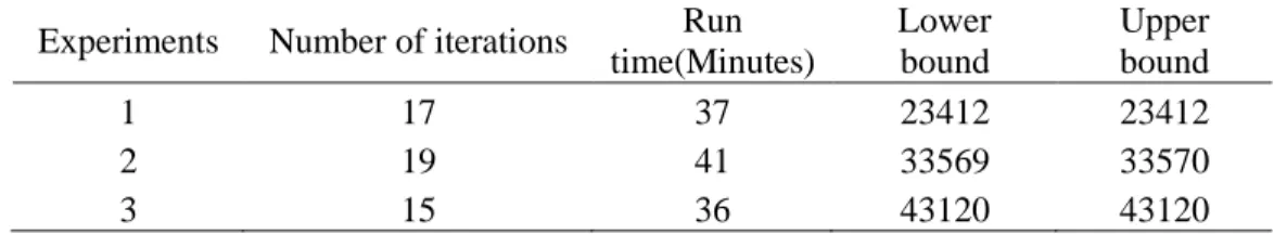
For three set of random parameters the model is solved by the proposed algorithm (Benders' decomposition) and the number of iterations for convergence of the model, running time and lower bound and upper bound of the solution is reported in table2.

Table 2. Numerical results for the three datasets

Experiments Number of iterations Run

time(Minutes)

Lower bound

Upper bound

1 17 37 23412 23412

2 19 41 33569 33570

3 15 36 43120 43120

The related experimental results are reported in figure 2, as the experimental results illustrated the running time of the bi-level model is appropriate for this large scale problem. Figure 2 shows the convergence of the model more clearly for three mentioned data sets.

Figure 2. Convergence of benders decomposition algorithm for experiments 1-3

23100 23200 23300 23400 23500 23600 23700

1 2 3 4 5 6 7 8 9 10 11 12 13 14 15 16 17

Iteration number

Experiment 1

33350 33400 33450 33500 33550 33600 33650 33700

1 2 3 4 5 6 7 8 9 10 11 12 13 14 15 16 17 18 19

Iteration number Experiment 2

42950 43000 43050 43100 43150 43200

1 2 3 4 5 6 7 8 9 10 11 12 13 14 15

Iteration number Experiment 3

(15)

44 6-2-

Impact of disruption

This section aims to examine the impact of considering disruption in competitive supply chain network design. First the model is solved without any disruption in distribution centers and transportation links and then disruptions are considered individually. The importance level of each disruption and their impact on the profit of producer and resellers is determined. As it has being illustrated in figure 3 the producer

Figure 3. Impact of Disruption

and also reseller's profits are reduced when disruption is considered in SCND, but the impact of the disruption on transportation links between DCs and resellers are more obvious on the profit of producer

while this disruption makes the resellers obtain more profit in comparison with other case of disruptions.

As it is obvious, disruption at DCs will be more effective on the performance of supply chain and decreases the profit of producer and resellers more visibly.

It can be concluded that each disruption has a different impact on the performance of supply chain and

considering these disruptions in SCND could cause recognizingthem easier.

6-3-

Considering competition

As mentioned before, the competition has been considered among producer and resellers. For analyzing the competition among them, the proposed model is solved first without considering the competition. For this purpose, each of objective functions is optimized and then the results are compared with competitive condition.

0 0.2 0.4 0.6 0.8 1 1.2 1.4

B

ilio

n

Profit of producer

1.59 1.6 1.61 1.62 1.63 1.64 1.65 1.66 1.67

B

ilio

n

Profit of Resellers

Disruption in transportation link between DCs and resellers

Disruption in transportation link between producer and DCs

(16)

45

Figure 4. Competition between Producer and resellers

As figure 4 illustrates when competition is considered, the leader decides for the location of new DCs and the price of products which makes the profit of resellers reduce. When more DCs are established the resellers are eager to provide their needs more form the producer which makes the profit of producer increase. So as a leader the producer should be considered the market's competitive environment to achieve more profits.

6-4-

Capacity of facilities

Now sensitivity analysis will be done to examine whether facility capacity adjustment can be used as a strategy to improve Profit for the leader or not. A general observation is that increased capacity of DCs

results in reduced supply chain costand increase in profit for leader. Similar patterns can be observed for

the three datasets. The cost savings (curve steepness) is indeed a function of “inventory cost over transportation cost” ratio. As figure 5 show, dataset 2 holds the lowest ratio implying a greater transportation cost and smaller inventory cost which allows the network to take advantage of increased capacity of facilities to reduce the frequency and quantity of shipments between supply chain nodes.

Figure 5. Analysis on capacity of facilities

0.875 0.88 0.885 0.89 0.895 0.9 0.905 0.91

B

ilio

n

Profit of producer

Considering Competition No Competition

2.135 2.14 2.145 2.15 2.155 2.16 2.165 2.17

B

ilio

n

Profit of resellers

Considering Competiton No Competition

0 0.5 1 1.5 2 2.5 3

0 0.1 0.2 0.3 0.4 0.5 0.6

P

ro

fi

t C

ha

nge

(%

)

Capacity change(%)

Set1 Set2 Set3

(17)

46 7-

Conclusion and future research

Competition and disruption both have a great impact on the correct performance of organizations and

firms. Small crash in systems could cause different kind of disruptionsand also can be seen as a severe

threat to the society and environment. Disruption in the supply chain components can cause a loss of market share in a competitive market and will create irreparable damages or harm. Therefore, taking possible disruptions into account in supply chains at the planning period could reduce costs, increase competitiveness, service and reliability. In this paper, a bi level programming was used to design a reliable competitive supply chain network by considering risk of disruption in distribution centers and communication links. The competition has been considered among two main components of the chain (the main provider agencies or retail-sales). Then the impact of each disruption and competition among supply chain members' has been investigated. Also Benders' decomposition algorithm was used for solving the proposed model and the efficiency of the proposed solution is investigated for large scale problem.

The modeling effort in this paper can set the stage for additional research in the area of competitive supply chain network design. Future researches could investigate the application of the model and solution method presented in this paper to manage actual supply chain challenges. In addition, more sophisticated models and solution techniques such as multi-objective programming and also robust optimization can be used for developing the presented model in this paper.

References:

Azad, N., & Davoudpour, H. (2013). Designing a stochastic distribution network model under risk. The

International Journal of Advanced Manufacturing Technology, 64(1-4), 23-40.

Ben-Ayed, O., Boyce, D. E., & Blair, C. E. (1988). A general bilevel linear programming formulation of the network design problem. Transportation Research Part B: Methodological, 22(4), 311-318.

Benders, J. F. (1962). Partitioning procedures for solving mixed-variables programming problems. Numerische mathematik, 4(1), 238-252.

Bernstein, F., & Federgruen, A. (2004). A general equilibrium model for industries with price and service competition. Operations research, 52(6), 868-886.

Bode, C., & Wagner, S. M. (2015). Structural drivers of upstream supply chain complexity and the frequency of supply chain disruptions. Journal of Operations Management, 36, 215-228.

Boyaci, T., & Gallego, G. (2004). Supply chain coordination in a market with customer service competition. Production and Operations Management,13(1), 3-22.

Cardona-Valdés, Y., Álvarez, A., & Ozdemir, D. (2011). A bi-objective supply chain design problem with uncertainty. Transportation Research Part C: Emerging Technologies, 19(5), 821-832.

Cardoso, S. R., Barbosa-Póvoa, A. P., Relvas, S., & Novais, A. Q. (2015). Resilience metrics in the assessment of complex supply-chains performance operating under demand uncertainty. Omega, 56, 53-73.

Drezner, Z. (1987). Heuristic solution methods for two location problems with unreliable facilities. Journal of the Operational Research Society, 509-514.

(18)

47

Fallah, H., Eskandari, H., & Pishvaee, M. S. (2015). Competitive closed-loop supply chain network design under uncertainty. Journal of Manufacturing Systems, 37, 649-661.

Farahani, R. Z., Rezapour, S., Drezner, T., Esfahani, A. M., & Amiri-Aref, M. (2014). Locating and capacity planning for retailers of a new supply chain to compete on the plane. Journal of the Operational

Research Society, 66(7), 1182-1205.

Farahani, R. Z., Rezapour, S., Drezner, T., & Fallah, S. (2014). Competitive supply chain network design: An overview of classifications, models, solution techniques and applications. Omega, 45, 92-118.

Giri, B. C., & Bardhan, S. (2015). Coordinating a supply chain under uncertain demand and random yield in presence of supply disruption.International Journal of Production Research, 53(16), 5070-5084.

Gurnani, H., Erkoc, M., & Luo, Y. (2007). Impact of product pricing and timing of investment decisions on supply chain co-opetition. European Journal of Operational Research, 180(1), 228-248.

Han, X., Chen, D., Chen, D., & Long, H. (2015). Strategy of Production and Ordering in Closed-loop Supply Chain under Stochastic Yields and Stochastic Demands. International Journal of u-and e-Service,

Science and Technology, 8(4), 77-84.

Hsu, C. I., & Li, H. C. (2011). Reliability evaluation and adjustment of supply chain network design with demand fluctuations. International Journal of Production Economics, 132(1), 131-145.

Jabbarzadeh, A., Fahimnia, B., & Sheu, J. B. (2015). An enhanced robustness approach for managing supply and demand uncertainties.International Journal of Production Economics.

Jabbarzadeh, A., Jalali Naini, S. G., Davoudpour, H., & Azad, N. (2012). Designing a supply chain network under the risk of disruptions. Mathematical Problems in Engineering, 2012.

Keyvanshokooh, E., Ryan, S. M., & Kabir, E. (2016). Hybrid robust and stochastic optimization for closed-loop supply chain network design using accelerated Benders decomposition. European Journal of

Operational Research, 249(1), 76-92.

Ko, H. J., & Evans, G. W. (2007). A genetic algorithm-based heuristic for the dynamic integrated forward/reverse logistics network for 3PLs. Computers & Operations Research, 34(2), 346-366.

Pan, F., & Nagi, R. (2010). Robust supply chain design under uncertain demand in agile manufacturing. Computers & Operations Research, 37(4), 668-683.

Park, S., Lee, T. E., & Sung, C. S. (2010). A three-level supply chain network design model with risk-pooling and lead times. Transportation Research Part E: Logistics and Transportation Review, 46(5), 563-581.

Peng, P., Snyder, L. V., Lim, A., & Liu, Z. (2011). Reliable logistics networks design with facility disruptions. Transportation Research Part B: Methodological, 45(8), 1190-1211.

Pishvaee, M. S., Razmi, J., & Torabi, S. A. (2014). An accelerated Benders decomposition algorithm for sustainable supply chain network design under uncertainty: A case study of medical needle and syringe supply chain.Transportation Research Part E: Logistics and Transportation Review, 67, 14-38.

(19)

48

Rezaee, A., Dehghanian, F., Fahimnia, B., & Beamon, B. (2015). Green supply chain network design with stochastic demand and carbon price.Annals of Operations Research, 1-23.

Rezapour, S., Allen, J. K., & Mistree, F. (2015). Uncertainty propagation in a supply chain or supply network. Transportation Research Part E: Logistics and Transportation Review, 73, 185-206.

Rezapour, S., & Farahani, R. Z. (2010). Strategic design of competing centralized supply chain networks for markets with deterministic demands.Advances in Engineering Software, 41(5), 810-822.

Rezapour, S., & Farahani, R. Z. (2014). Supply chain network design under oligopolistic price and service level competition with foresight. Computers & Industrial Engineering, 72, 129-142.

Romeijn, H. E., Shu, J., & Teo, C. P. (2007). Designing two-echelon supply networks. European Journal

of Operational Research, 178(2), 449-462.

Sadghiani, N. S., Torabi, S. A., & Sahebjamnia, N. (2015). Retail supply chain network design under operational and disruption risks. Transportation Research Part E: Logistics and Transportation

Review, 75, 95-114.

Saharidis, G. K., & Ierapetritou, M. G. (2009). Resolution method for mixed integer bi-level linear problems based on decomposition technique. Journal of Global Optimization, 44(1), 29-51.

Santoso, T., Ahmed, S., Goetschalckx, M., & Shapiro, A. (2005). A stochastic programming approach for supply chain network design under uncertainty. European Journal of Operational Research, 167(1), 96-115.

Seifert, R. W., & Langenberg, K. U. (2011). Managing business dynamics with adaptive supply chain portfolios. European Journal of Operational Research, 215(3), 551-562.

Shen, Z. J. M. (2005). A multi-commodity supply chain design problem. IIE Transactions, 37(8), 753-762.

Shen, Z. J. M., & Daskin, M. S. (2005). Trade-offs between customer service and cost in integrated supply chain design. Manufacturing & Service Operations Management, 7(3), 188-207.

Snyder, L. V., & Daskin, M. S. (2005). Reliability models for facility location: the expected failure cost case. Transportation Science, 39(3), 400-416.

Sun, H., Gao, Z., & Wu, J. (2008). A bi-level programming model and solution algorithm for the location of logistics distribution centers. Applied mathematical modelling, 32(4), 610-616.

Torabi, S. A., Baghersad, M., & Mansouri, S. A. (2015). Resilient supplier selection and order allocation under operational and disruption risks.Transportation Research Part E: Logistics and Transportation

Review, 79, 22-48.

Üster, H., & Agrahari, H. (2011). A Benders decomposition approach for a distribution network design problem with consolidation and capacity considerations. Operations Research Letters, 39(2), 138-143. Vidal, C. J., & Goetschalckx, M. (2001). A global supply chain model with transfer pricing and transportation cost allocation. European Journal of Operational Research, 129(1), 134-158.

(20)

49

Viswanadham, N., & Gaonkar, R. S. (2003). Partner selection and synchronized planning in dynamic manufacturing networks. Robotics and Automation, IEEE Transactions on, 19(1), 117-130.

Xiao, T., & Yang, D. (2008). Price and service competition of supply chains with risk-averse retailers under demand uncertainty. International Journal of Production Economics, 114(1), 187-200.

Xu, J., Liu, Q., & Wang, R. (2008). A class of multi-objective supply chain networks optimal model under random fuzzy environment and its application to the industry of Chinese liquor. Information

Sciences, 178(8), 2022-2043.

Yin, S., Nishi, T., & Grossmann, I. E. (2015). Optimal quantity discount coordination for supply chain optimization with one manufacturer and multiple suppliers under demand uncertainty. The International

Journal of Advanced Manufacturing Technology, 76(5-8), 1173-1184.

You, F., & Grossmann, I. E. (2008). Design of responsive supply chains under demand uncertainty. Computers & Chemical Engineering, 32(12), 3090-3111.

Yu, H., Zeng, A. Z., & Zhao, L. (2009). Single or dual sourcing: decision-making in the presence of supply chain disruption risks. Omega, 37(4), 788-800.

Zhang, D. (2006). A network economic model for supply chain versus supply chain competition. Omega, 34(3), 283-295.

Zhang, L., Rushton, G., 2008. Optimizing the size and locations of facilities in competitive multi-site

service systems. Computers & Operations Research (35), 327-338.

Appendix A

In this section the constraints of SP2 (Slave problem 2) for KKT optimality condition are given: