ORIGINAL ARTICLE
Forecasting Farm-Gate Catfish Prices in Uganda Using SARIMA Model
James O. Bukenya Alabama A&M University
Abstract: Stabilization of prices of essential agricultural commodities continues to remain an area of major concern for policy makers; given that price instability affects both producers and consumers, and has macroeconomic implications. This paper examines farm-gate price behavior in the African catfish markets in Uganda, and develops a forecasting model that adjusts for the seasonal fluctuations in the price series. The analysis utilizes monthly catfish real price series for the period January 2006 to December 2013. The model provides good in-sample and out-of-sample forecasts for the eight-year time period. The out-sample predictions based on SARIMA (1, 1, 1) (0, 1, 1)12model suggest that the stochastic seasonal fluctuations depicted in the price series are successfully modeled, and that catfish real prices follow an upward trend. The findings can assist policy makers and major stakeholders to gain insight into more appropriate economic and sectorial policies that can lead to the development of reliable market information systems and up-to-date data on catfish supply, demand and stocks.
Keywords: SARIMA models; Box – Jenkins; Forecasting; catfish prices; Uganda
1. Introduction
Over the last decade, aquaculture has emerged as a vibrant subsector in Uganda, with its share in total fish production increasing substantially[1]. With increasing market prices, government intervention for increased production, and stagnating supply from capture fisheries, aquaculture has attracted entrepreneur farmers seeking to exploit the business opportunity provided by the prevailing fish demand. The bulk of the increase in aquaculture production has been attributed to the African catfish (Clariasgariepinus) which accounts for more than 65% of aquaculture production in Uganda. African catfish farming is flourishing mostly due to its relatively developed production technology, emerging new markets in the region, and the growing middle class in Uganda. Its market is sustained by the relatively consistent supply from farms. Although production has increased over time, fish prices in general have remained highly unstable, a phenomenon that could potentially explain why fish producers are operating at narrow net margins. Basic economic theory suggests that the role which the price mechanism is expected to perform does not materialize in a highly unstable price situation. In such instances, price fluctuation translate into significant price risk, since the magnitude and the direction of the price changes are often unknown to producers; hence, making the timing of production extremely important. As an illustration, selling 5kg fish in November for UGX 2257 per kilogram will bring losses, whereas, selling the same fish in June for UGX 2410 per kilogram may be very profitable. Therefore, farmers have to frequently assess whether to harvest to capture a known price, or to continue to feed to deliver a larger fish at an unknown future price[2].This has increased the risk faced by fish producers in general, and catfish farmers in particular. The objective of this paper therefore, is to develop a forecasting model that would allow catfish farmers in Uganda to make better-informed decisions and to manage price risk.
Copyright © 2017 James O. Bukenya doi: 10.18686/fm.v2i2.1047
This is an open-access article distributed under the terms of the Creative Commons Attribution Unported License
(http://creativecommons.org/licenses/by-nc/4.0/), which permits unrestricted use, distribution, and reproduction in any medium, provided the original work is properly cited.
Price forecasting in fisheries and aquaculture has been the subject of a wide range of studies which have used a variety of approaches, ranging from simple to more complex forecasting models. Relevant studies include Curtis,
Ligeon and Hishamunda [3]who used autoregressive conditional heteroscedastic (ARCH) models and the generalized
autoregressive conditional heteroscedastic (GARCH) with ordinary least squares (OLS), unconditional least squares (ULS), and maximum likelihood (ML) models to forecast whole and frozen catfish prices in the U.S. Similarly, Guttormsen[4]used classical additive decomposition (CAD), Holt-Winters exponential smoothing (HW), auto-regressive moving average (ARMA), vector auto-regression (VAR) and two different naïve models to forecast weekly producer
prices for salmon in Norway. Gordon[5]used ARMAX model to provide a parsimonious characterization of producer
prices and simulated price effects from exchange rate shocks in Canada. Gu and Anderson[6] used an approach that
combines seasonality removal with a multivariate, state-space time series forecasting model to provide short-run forecasts for the U.S. salmon market. Prista et al.[7]used seasonal autoregressive integrated moving average (SARIMA) models to fit, forecast, and monitor meagre landings in Portugal. This paper contributes to this body of knowledge by developing a SARIMA model to forecast farm-gate catfish prices in Uganda.
2. Materials and Methods
Forecasting Framework
During the past few decades, much effort has been devoted to the development and improvement of time series forecasting models[3-7]. One of the most important and widely used time series models is the Auto-Regressive Integrated Moving Average (ARIMA) model. The popularity of the ARIMA model is due to its statistical properties, as well as, use of well-known Box-Jenkins methodology in the model building process. In general, an ARIMA model is characterized by the notation ARIMA (p, d, q), where p, d and q denote orders of Auto-Regression (AR), Integration (differencing) and Moving Average (MA), respectively. An ARMA (p, q) process can be defined as:
q t q t
t t p t t
t
t
c
y
y
y
1 1
2 2
...
1
1
2
2
...
(1)Where, ytand εtare the actual value and random error at time period t, respectively,
i(i=1, 2, p) and
j(j=1, 2… q) are the model parameters. The random errors, εt are assumed to be independently and identically distributed with amean of zero and a constant variance of σ2.The Seasonal Auto-Regressive Integrated Moving Average (SARIMA)
model is an extension of the ARIMA model, which not only captures regular difference, autoregressive, and moving average components as the ARIMA model, but also handles seasonal behavior of the time series. In the SARIMA model, both seasonal and regular differences are performed to achieve stationarity prior to fitting the model.
To solve the problem of the seasonal character of catfish price series, SARIMA model is proposed here, which includes trend, seasonal component, and short-time adjustments. The model is derived from the standard Box-Jenkins model [8, 9]. SARIMA models include seasonal and non-seasonal factors in the multiplicative model according to the following formula:
t s Q t
s
P
(
B
)
Z
(
B
)
a
(2)
the backshift operator. Seasonal differencing may be in order if the seasonal component follows a random walk, as in: t s s t t
t
Z
Z
B
Z
Z
(
)
1
(3)The seasonal difference of order D is defined as:
t D s t
D
S
Z
(
B
)
Z
1
(4)So the final form of SARIMA (p, d, q) x (P, D, Q)scan be formed as:
t q s Q t d D s p s
P
(
B
)
(
B
)
Z
(
B
)
(
B
)
a
(5) Where Ps P s s sP
B
B
B
B
(
)
1
1 2 2...
p p
p
B
B
B
B
(
)
1
1
2 2
...
Qs Q s
s s
Q
B
B
B
B
(
)
1
1 2 2...
q q
q
B
B
B
B
(
)
1
1
2 2
...
In the current study, the focus is on monthly catfish price series and since the seasonal period of the series s = 12, equation (5) can be rewritten as:
t q Q t d D p
P
(
B
12)
(
B
)
12
Z
(
B
12)
(
B
)
a
(6) where
p(
B
)
is the autoregressive stationary operator (non-seasonal) of order p;
P(
B
12)
is the autoregressivestationary operator of order P and seasonal station 12;
q(
B
)
is the operator of invertible moving average(non-seasonal) of order q;
Q(
B
12)
is the seasonal invertible of moving average operator of order Q and seasonal station 12;
d is the part of non-seasonal integration order d;
12D is the part of seasonal integration order D and seasonal station 12.3. Data Description
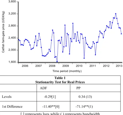
The analysis utilizes an updated data sample[10-12]of monthly average catfish prices covering the period January 2006 through December 2013. The data are taken from secondary source recorded data by the Aquaculture Management Consultant[13].To adjust for inflation, catfish prices, expressed in Uganda Shillings (UGX) per kilogram (kg), were deflated using a consumer price index (CPI) deflator from the Uganda Bureau of Statistics[14]. The deflated series is plotted in Figure 1, showing consistent pattern of short-term changes, which is an indication of non-stationarity of the time series. The sharp decreases observed annually during the months of February, August and December suggests the possibility of some seasonal component that could also make catfish price series non-stationary. For further testing of the stationarity of the price series, Augmented Dickey Fuller (ADF) and Phillips-Perron (PP) unit root test statistics are
applied. The optimal number of lags is determined using the Schwarz information criteria. The unit root test results are reported in Table 2, confirming that the hypothesis of non-stationarity cannot be rejected at the 5% significance level.
Figure 1. Monthly catfish farm-gate real prices
1,600 2,000 2,400 2,800 3,200 3,600
2006 2007 2008 2009 2010 2011 2012 2013
C at fis h fa rm -g at e pr ic e (U G X/ kg )
Time period (monthly)
Table 1
Stationarity Test for Real Prices
ADF PP
Levels -0.29[1] 0.34 (13)
1st Difference -11.40**[0] -71.14**(1)
[ ] represents lags while ( ) represents bandwidth 0.05 critical values: -2.89
Lag Length- based on SIC, maxlag=11.
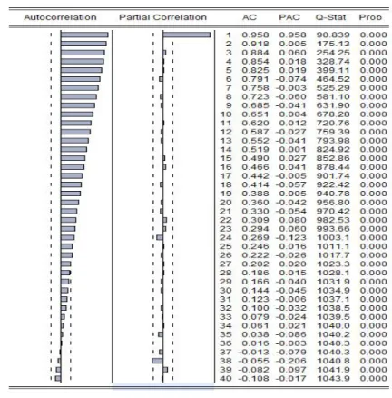
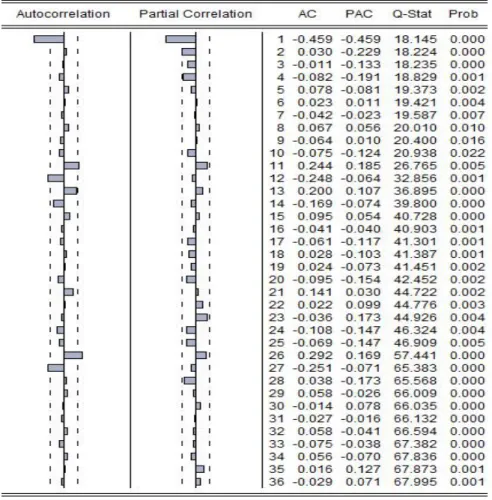
Investigation is also done by examining the autocorrelation (ACF) and partial autocorrelation (PACF) functions (Figure 2). As shown in the figure, the ACF dies down extremely slowly, while the PACF cuts off after the first lag. Overall, the unit root test results and plots of the correlogram confirm that the time series price data are not stationary, and thus need some treatments to be transformed to a stationary series. Accordingly, the first difference of the series is examined (Table 2), and the test results confirm that catfish real price series is integrated of order 1 or I(1). The plot of the first differenced series is displayed in Figure 3, showing that the differenced series is stationary but shows some seasonal patterns. The next step was to examine the behavior of the seasonal patterns in the data using the seasonal unit root test.
Figure 3. Time Series Plot of First Differences of Monthly Catfish Real Price Series
-1,200 -800 -400 0 400 800 1,200
2006 2007 2008 2009 2010 2011 2012 2013
Fi rst D iff ere nc e o f R ea l P ric e S eri es
Figure 2. Correlogram of Original Catfish Real Price Series
4. Seasonal Unit Root Test
The most common approach used to determine if the seasonal behavior in the data series is deterministic, stochastic or stationary under seasonal frequencies is the HEGY approach[15]. As extended by Franses[16], the seasonal frequencies in the data series are π, π/2, 2π/3, π/3, 5π/3 and π/6. Testing for both seasonal and non-seasonal unit roots is also implied in testing for the significance of πi. The t-test is used to test the separate π’s of the null hypothesis. It is a one sided t-test that πi= 0 and π2= 0 of the null hypothesis, respectively. The two sided t-test are used in testing for the null hypothesis of πi= 0, i = 3,...,12 The F-statistic is used to test for the joint null hypothesis that π2, π3, and π4are all zero and that all four π’s are jointly zero (π1=π2=π3=π4=0). The asymptotic distribution of the test statistics under the respective null
hypothesis depend on the deterministic terms in the model. There is no seasonal unit root if π2through π12 are
significantly different from zero. If π1=0, then the presence of non-seasonal unit root cannot be rejected. Table 2 presents the results from the HEGY test, suggesting that, the null hypothesis of unit root at the non-seasonal frequency cannot be rejected while the presence of unit root at the seasonal frequency can be rejected at the 5% level only for three seasonal frequencies (π, 2π/3 and 5π/3). The failure to reject the null hypothesis of unit root at the rest of the seasonal frequencies implies the presence of some seasonal components in the catfish real price series, thus raising the need to perform seasonal differencing on the price series.
Table 2
HEGY Seasonal Unit Root Test Results for Real Catfish Prices
Auxiliary Regression Seasonal Frequency StatisticsTest SimulatedP-value* 5% Critical values^
t-test: π1=0 0 -2.34 0.32 -3.19
t-test: π2=0 π -4.10 0.01 -2.65
F-test: π5=π6=0 2π/3 8.81 0.00 5.77
F-test: π7=π8=0 π/3 5.17 0.06 5.77
F-test: π9=π10=0 5π/3 5.73 0.03 5.84
F-test: π11=π12=0 π/6 4.96 0.07 5.82
*Monte Carlo Simulations: 1000 Selected lag using aic criteria: 2 ^Franses and Hobijn[17]
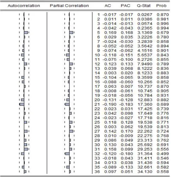
The next step in the Box and Jenkins procedure is to determine the order of the AR and MA for seasonal and non-seasonal components. This is accomplished using the sample ACF and PACF plots of the price series. Earlier examination of the ACF plot in Figure 2 revealed that the ACF declines very slowly while the PACF showed a single spike at the first lag. These observations suggest p=1 and q=1 as starting points in describing the catfish real price series as coming from a non-seasonal AR and MA process, respectively. Hence, the model that gives rise to these observations is an ARIMA (1, 1, 1) model, since the data series was differenced (i.e.d=1) to attain stationarity. Similarly, the plot of the ACF and PACF of the seasonally differenced series is presented in Figure 4. A critical look at the seasonal lags shows that the ACF spikes at seasonal lag 12 dies down to zero for other seasonal lags, while the PACF shows no spike at any of the seasonal lags, suggesting that p=0 and q=1 would be needed to describe these data as coming from a seasonal autoregressive and moving average process. Hence, the time series model that gives rise to these observations is an ARIMA (0, 1, 1) model, since the data are seasonally differenced once (i.e. d=1) to address the presence of seasonal frequencies as indicated by the HEGY seasonality test in Table 2. Overall, the first guess model based on these observations is SARIMA (1, 1, 1) (0, 1, 1)12.The model is estimated along with other possible models and the Akaike Information Criterion (AIC) and Schwarz Bayesian Information Criterion (BIC)are used to select the best model.
5. Identification of the SARIMA Model
In the identification phase, six tentative SARIMA models are tested and the corresponding AIC, AICC and BIC values for each of the models are presented in Table 3. The results show that SARIMA (1, 1, 1) (0, 1, 1)12has the least AIC, AICC and BIC values, and thus presented as the best model. The next stage of the Box-Jenkins approach is the estimation of parameters of the selected model.
Table 3
Postulated SARIMA Models and Performance Evaluation
SARIMA Model # of estimated parameters AIC (F-corrected-AIC)AICC BIC
(0,1,0) (0,1,1) 2 1182.57 1182.72 1187.41
(0,1,0) (1,1,0) 2 1199.47 1199.62 1204.31
(0,1,1) (0,1,1) 3 1180.70 1181.01 1187.96
(0,1,1) (1,1,0) 3 1192.63 1192.93 1199.89
(1,1,0) (0,1,1) 3 1181.97 1182.28 1189.23
(1,1,0) (1,1,0) 3 1195.13 1195.43 1202.39
(1,1,1) (0,1,1) 4 1178.74 1179.26 1187.42
Figure 4. Correlogram of the Seasonally Differenced Monthly Catfish Prices
6. Parameter Estimation
The parameters of SARIMA (1, 1, 1) (0, 1, 1)12 are estimated using the maximum likelihood estimator in Eviews
Version 7.2. As reported in Table 4, the coefficient of the estimated ARIMA and the seasonal MA parameters are 0.6532, 0.9012 and 0.8095, respectively. Based on 95% confidence level, it can be concluded that all the coefficients of the SARIMA (1, 1, 1) (0, 1, 1)12model are significantly different from zero.
Table 4
Estimated Parameters of SARIMA (1, 1, 1)(0, 1, 1)12 Model
Parameter Estimate Standard Errors t-Value
Nonseasonal AR
Lag 1 0.6532* 0.12170 5.3767
Nonseasonal MA
Lag 1 0.9012* 0.07270 12.3962
Seasonal MA
Lag 12 0.8095* 0.07984 10.1390
Variance 0.66652E+05
Likelihood Statistics
Effective number of observations (nefobs) 83
Log likelihood (L) -585.3719
AIC 1178.7438
AICC (F-corrected-AIC) 1179.2566
Hannan Quinn 1182.6308
BIC 1187.4192
7. Model Validation
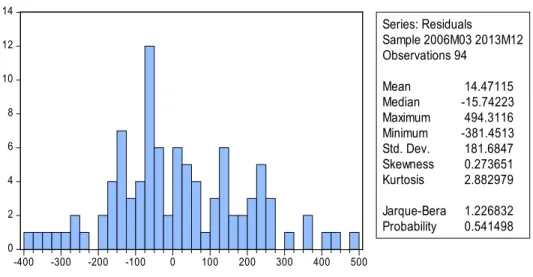
Model verification stage of the Box-Jenkins approach is concerned with checking the residuals of the estimated model to determine if the model contains any systematic pattern, which can be removed to improve on the selected SARIMA model. Verification is tested by verifying the PACF of the residuals and the normal probability plot of the residuals. Figure 5presents the correlogram of residual of the series, indicating that there is no significant spike of PACF. This means that the residual of SARIMA (1, 1, 1) (0, 1, 1)12model are white noise. That is, the residuals have zero mean, constant variance and also uncorrelated. The p-vales for the Ljung-Box statistic clearly all exceed 5% for all lag orders, implying that there is no significant departure from white noise for the estimated residuals. Furthermore, Figure 6 presents the histogram of the estimated residuals and the associated statistics. The reported Jarque–Bera test for normality of the residuals is estimated to be 1.227, which is less than the critical value of chi–square distribution at 5% level of significance. Based on the Jarque–Beratest, the null hypothesis of normality cannot be rejected. Once the model diagnostic tests showed that all the estimated parameters are significant and the residual series are random, it was concluded that SARIMA (1, 1, 1) (0, 1, 1)12model is adequate for forecasting catfish real prices.
Figure 6. Histogram of the Residuals of Fitted SARIMA Model
0 2 4 6 8 10 12 14
-400 -300 -200 -100 0 100 200 300 400 500
Series: Residuals
Sample 2006M03 2013M12 Observations 94
Mean 14.47115 Median -15.74223 Maximum 494.3116 Minimum -381.4513 Std. Dev. 181.6847 Skewness 0.273651 Kurtosis 2.882979 Jarque-Bera 1.226832 Probability 0.541498
8. Model Forecasting
The selected SARIMA (1, 1, 1) (0, 1, 1)12model is used to conduct both in-sample and out-sample forecasts for catfish prices in Uganda. Thus, the first forecast (for January to December 2012) is constructed based on in-sample estimation using the period January 2006 to December 2012. The one-year in-sample size is chosen arbitrarily. The predicted catfish prices are then compared with the observed catfish prices (Table 5). From the table, it can be noticed that most of the predicted catfish real prices are close to the observed prices. Moreover, all the actual prices fall within the 95% confidence intervals of the forecasts, which confirms that the model provides an acceptable fit to predict monthly catfish real prices.
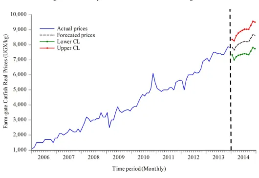
The out-sample forecast is conducted using the full data sample from January 2006 to December 2013. Table 6 presents the forecasts for January to December 2014, and Figure 7 plots the forecasted prices. As depicted in Figure 7, SARIMA (1, 1, 1,) (0, 1, 1)12 model predicts a continued upward trend observed in the historical price series. The accuracy of the model is evaluated based on the mean absolute percentage error (MAPE), the root-mean-square error (RMSE), and the mean absolute error (MAE). A mere glance at the results in Table 7 clearly indicates that the model is correctly specified for the purpose of forecasting. For instance, MAPE results suggest that the model can forecast catfish real prices within an accuracy of 4.9%, meaning that the forecast are off by about 5% on average.
Table 5
Actual and In-sample Predicted Prices (UGX/kg)for SARIMA (1,1,1) (0,1,1)12Model
Month (UGX/kg)Actual (UGX/kg)Forecast LCL UCL Month (UGX/kg)Actual (UGX/kg)Forecast LCL UCL
2013.Jan 7100 6941 6361 7521 2013.Jul 7450 7426 6854 7997
2013.Feb 6900 6965 6371 7560 2013.Aug 7350 7435 6867 8002
2013.Mar 7200 7000 6404 7595 2013.Sep 7352 7369 6802 7936
2013.Apr 7500 7211 6635 7788 2013.Oct 7614 7386 6819 7953
2013.May 7500 7446 6872 8019 2013.Nov 7871 7660 7075 8245
Table 6
Out-sample Predicted Real Prices [SARIMA (1,1,1) (0,1,1)12
Month Forecast(UGX/kg) LCL UCL
2014.Jan 7844.20 7338.20 8350.21
2014.Feb 7636.82 7003.70 8269.93
2014.Mar 7903.72 7203.75 8603.69
2014.Apr 8040.49 7298.88 8782.11
2014.May 8113.11 7342.33 8883.90
2014.Jun 8170.29 7377.10 8963.48
2014.Jul 8225.60 7413.92 9037.28
2014.Aug 8204.34 7376.54 9032.13
2014.Sep 8189.48 7347.08 9031.87
2014.Oct 8437.01 7581.02 9293.01
2014.Nov 8684.21 7815.29 9553.13
2014.Dec 8623.84 7742.49 9505.19
Table 7
Forecast Performance for SARIMA (1,1,1) (0,1,1)12Model
Root Mean Square Error 264.02
Mean Absolute Error 180.55
Mean Absolute Percent Error 4.909 Theil Inequality Coefficient 0.029
Bias Proportion 0.076
Variance Proportion 0.003
Covariance Proportion 0.922
Figure 7. Out-Sample Forecast for Catfish Prices in Uganda
9. Conclusions
Basic economic theory suggests that the behavior of agricultural commodity prices over time is governed by shifts in supply and demand. In particular, deviations of actual production from expected supplies can have a pronounced impact
on price patterns. This is particularly true for emerging agricultural sectors in developing countries like the aquaculture subsector in Uganda. The objective here was to develop a forecasting model to examine the behavior of farm-gate real prices in the catfish markets and to predict future prices using historical time series data from January 2006 to December 2013. To this end, a SARIMA (1, 1, 1) (0, 1, 1)12model that incorporate the seasonality of the time series was developed and tested. The results indicated that the model fitted the data well and that the stochastic seasonal fluctuations manifest in the data series were successfully modeled. Model predictions indicated that catfish real prices in Uganda continues to follow an increasing trend with stochastic seasonal effects. The mean absolute percentage error suggested that the estimated model can predict catfish real prices with an accuracy of 4.9%. As a way forward, these findings can help policy makers and other major stakeholders gain insights into more appropriate economic and sectorial policies that can lead to reliable market information system and up-to-date information on supply, demand and stocks. As others have noted, an adequate fish stock is a necessary component of a well-functioning market, in particular, to smooth out seasonal fluctuations and time lags in fish trade.
Limitation:The data used in this analysis are for a period of eight years, which is limited for complex time series
models. Furthermore, the subsector examined is prevalent with market imperfections at the production, harvesting, and marketing levels, hence, caution should be exercised when drawing broader conclusions from the results. Despite the limitations, it is undeniable that price forecast is essential, even in such highly imperfect markets.
10. Acknowledgments
This research is a component of AquaFish Innovation Lab, supported by USAID (CA/LWA No. EPP-A-00-06-00012 -00) and by contributions from the participating institutions. The AquaFish succession number 1477. The opinions expressed herein are those of the author and do not necessarily reflect the views of AquaFish or the U.S. Agency for International Development.
References
1. FAO/FishStat (2016). National Aquaculture Sector overview: Uganda. Retrieved July 10, 2017, from
http://www.fao.org/fishery /countrysector/naso_uganda/en.
2. Forsberg, O.I., & A.G.Guttormsen (2006). The value of information in salmon farming. Harvesting the right fish at the right
time. Aquaculture Economics & Management, 10:183–200.
3. Curtis M. J., C. Ligeon& N. Hishamunda (1998). Forecasting catfish industry prices using linear and nonlinear methods.
Aquaculture Economics & Management, 2(2): 71-80.
4. Guttormsen, A. G. (1999). Forecasting weekly salmon prices: Risk management in fish farming. Aquaculture Economics and
Management, 3 (2): 159–166.
5. Gordon, D.V. (2017). Price modelling in the Canadian fish supply chain with forecasts and simulations of the producer price of
fish. Aquaculture Economics & Management, 21(1): 105-124.
6. Gu, G., &J.L. Anderson (1995). Deseasonalized state-space time-series forecasting with application to the U.S. salmon market.
Marine Resource Economics, 10: 171–185.
7. Prista, N., N. Diawara, M.J Costa& C. Jones (2011). Use of SARIMA models to assess data-poor fisheries: A case study with a
sciaenid fishery off Portugal. Fishery Bulletin, 109(2): 170-185.
8. Box, G.E.P. & G.M. Jenkins (1970). Time series analysis; Forecasting and control. Holden-Day, San Francisco (CA).
9. Box, G. E. P. & G. M. Jenkins (1976). Time series analysis: Forecasting and control. Revised edition, San Francisco: Holden
Day.
10. Bukenya, J.O., & M. Ssebisubi (2014). Price integration in the farmed and wild fish markets in Uganda. Fisheries Science, 80 (6): 1347-1358.
11. Bukenya, J.O., & M. Ssebisubi (2015). Price transmission and threshold behavior in the African catfish supply chain in Uganda.” Journal of African Business, 16(1-2): 180-197.
12. Bukenya, J.O. (2017). Assessment of price volatility in the fisheries sector in Uganda. Journal of Food Distribution Research, XLVIII (1): 81–88.
13. AMC. (2013). Aquaculture Management Consultant Ltd (Kampala: Uganda).
14. UBoS. (2013). Uganda Bureau of Statistics. Statistical abstracts 1995-2013. Retrieved September 17, 2013, from http://www.ubos.org/index.php.
15. Hylleberg, S., R.F. Engle, C.W.J Granger & B.S. Yoo (1990). Seasonal integration and cointegration. Journal of Econometrics, 44: 215–238.
16. Franses, P. H. (1991). Seasonality, nonstationarity and the forecasting of monthly time series. International Journal of Forecasting, 7: 199–208.
17. Franses, P.H., & B. Hobijn (1997). Critical values for unit root tests in seasonal time series. Journal of Applied Statistics, 24 (1):25-47.