An algorithm for integrated worker assignment, mixed-model
two-sided assembly line balancing and bottleneck analysis
Parvaneh Samouei
1*, Parviz Fattahi
21
Department of Industrial Engineering, Faculty of Engineering, Bu-Ali Sina University, Hamedan, Iran
2
Department of Industrial Engineering, Alzahra University, Tehran, Iran
[email protected],[email protected]
Abstract
This paper addresses a multi-objective mixed-model two-sided assembly line balancing and worker assignment with bottleneck analysis when the task times are dependent on the worker’s skill. This problem is known as NP-hard class, thus, a hybrid cyclic-hierarchical algorithm is presented for solving it. The algorithm is based on Particle Swarm Optimization (PSO) and Theory of Constraints (TOC) and consists of two stages. In stage one, simultaneous balancing and worker assignment are studied. In stage two, bottleneck analysis and product-mix determination are carried out. In addition, a bi-level mathematical model is presented to describe the problem. The following objective functions are verified in this paper: (1) minimizing the number of mated-stations (2), minimizing the number of stations (3) minimizing the human costs (4) minimizing the weighted smoothness index and (5) maximizing the total profit. In addition to the proposed algorithm, another algorithm, which is based on the simulated annealing and the theory of constraints, is developed to compare the performance of the proposed algorithm in terms of the running time and the solution quality over the different benchmarked test problems. Moreover, several lower bounds are developed for the number of the stations and the number of the mated-stations. The results show and support the efficiency of the proposed approaches.
Keywords:
Two-sided assembly line balancing problem (TSALBP), workerassignment, mixed-model, particle swarm optimization algorithm (PSO), simulated annealing algorithm (SA), theory of constraints.
1-Introduction
An assembly line is a production process that usually has several stations connected with a material handling device such as a conveyor belt. In this line, the unfinished products are launched down through the stations and a set of tasks with certain operation times and ordered relationships between them are carried out by robots or humans.
Salveson (1955) is the first author that introduced assembly line balancing problem (ALBP).Since then; many others have studied it with different constraints, objectives and solving methods in order to make better decisions in real-world situations. Several good surveys and taxonomies were published on ALBP in Scholl and Becker (2006), Boysen et al. (2007, 2008), Hu et al. (2011) and Battaïa and Dolgui (2013).
*Corresponding author
ISSN: 1735-8272, Copyright c 2018 JISE. All rights reserved Journal of Industrial and Systems Engineering
Vol. 11, No.2, pp. 151-174 Spring (April) 2018
There are several classifications for ALBP. Based on the number of the product models that are assembled in a line, this problem is divided into single, mixed and multi-models. In the single-model, one type of product is assembled. In the mixed-model several models of one type of product and in the multi-model, different product types in batches are assembled. Through these lines, the mixed-model assembly lines can reduce inventories, eliminate transfer costs among the mixed-models and meet ever-changing customer demands more efficiently (Hu et al. (2011)). Therefore, many factories use these assembly lines for their productions.
According to the properties of the products, the technical or operational requirements, layouts of the assembly lines can be one-sided, two-sided or U-shaped. In one-sided assembly lines, only one side of the line (right or left) is used; whereas, in the two-sided assembly line, both sides of the line are utilized. Since a two-sided line often has a shorter length, low-cost tools, fixtures and fewer material handling systems, this layout is used for large-sized products.
There are two famous objective functions for solving a two-sided assembly line balancing problems (TSALBP). Minimization of the number of the mated-stations (i.e., the line length) for a given time cycle is the Type-I and minimization of the cycle time for a given number of the mated-stations is the Type-II (Özcan and Toklu (2009)). Since the number of the stations for the same number of the mated-stations in Type-I can be different, the number of the mated-stations as well as the number of the stations may be verified in TSALBP.
According to the number of the objective function(s), TSALBP can be categorized based on one objective or multi-objective. For example, Xiaofeng et al. (2010) used one objective function and Simaria and Vilarinho (2009) had more than one objective in his research.
Similar to the one-sided ALBP, TSALBP is an NP-hard problem (Bartholdi (1993)). Therefore, metaheuristic algorithms, such as simulated annealing )Özcan et al. (2010)), Genetic Algorithm (Purnomo et al. (2013)), Ant Colony Optimization (ACO) (Simaria and Vilarinho (2009)) and Particle Swarm Optimization (Chutima and Chimklai (2012)) are used to solve the TSALBP in reasonable time to obtain optimal or near-optimal solutions.
Most of the research in ALBP assume that the operation times are deterministic (Hamta et al. (2013)), and do not depend on the worker’s skill. However, in many real-world situations, the task times depend on the worker’s skill. It is clear that when a worker is high-skilled, he (she) can do the specified task faster than a low-skilled worker. Thus, the worker’s skill can affect the line balancing. In addition, distinguishing between the levels of skills permits a manager to decide which tasks should be done by a worker. Therefore, verifying the worker assignment in ALBP is necessary and several researchers have investigated this problem in their papers. For example, Miralles et al. (2008) defined a mathematical model for the assembly line worker assignment and balancing problem and presented a basic branch and bound (B&B) approach with three possible search strategies and different parameters to solve it. Costa and Miralles (2009) verified the effect of the job rotation in this problem and proposed a metric along with a mixed integer linear model and a heuristic algorithm. Furthermore, Blum and Miralles (2011) solved this problem with beam search. Their model's objective was cycle time minimization for the fixed number of stations and workers.
Mutlu et al. (2013) considered the workers’ assignment and ALBP when task times depended on the skills of the operators and developed an iterative genetic algorithm to minimize the cycle time.
Zhang et al. (2008) addressed a Multi-Objective Genetic Algorithm (MOGA) for ALBP with worker allocation to, simultaneously, minimize (1) the cycle time (2) the variation of workload, and (3) the total cost. Moreover, Zaman et al. (2012) used a heuristic and an MOGA for assigning the operators to the predefined stations of an assembly line to get the sustainable result of fitness function of cycle time, the total idle time and the output.
A mixed integer programming model, a heuristic algorithm based on beam search, a task-oriented branch and a bound procedure, which used new reduction rules and lower bounds for solving worker assignment and balancing problems, are presented in Borba and Ritt (2014). Moreover, this problem led to the development of an exact enumeration algorithm for solving the problem (Vilà and Pereira (2014)).
Kellegöz (2017) presented a new mathematical formulation and Gantt based heuristic method for assembly line balancing problems with multi-manned stations. Also, Giglio et al. (2017) presented a new mathematical formulation for multi-manned assembly line balancing problem with skilled workers which allowed the workers in each multi-manned workstation to perform the different
assembly tasks of same product simultaneously to minimize the total operating cost of the assembly line. Furthermore, Roshani and Giglio used simulated annealing algorithms for the multi-manned assembly line balancing problem to minimize cycle time. Recently, Cannas et al. (2018) verified complexity reduction and kaizen events to balance manual assembly lines. Moreover, Dolgui et al. (2018) studied optimal workforce assignment to operations of a paced assembly line where workers can move among stations to adapt workstation capacities to workloads.
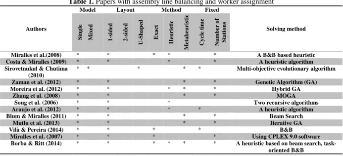
Table 1. Papers with assembly line balancing and worker assignment
Authors
Model Layout Method Fixed
Solving method S in g le M ix ed 1 -si d ed 2 -si d ed U -S h a p ed E x a ct Heuri st ic M et a h eu ri st ic C y cl e ti me N u mber o f S ta ti o n s
Miralles et al.(2008) * * * * * A B&B based heuristic
Costa & Miralles (2009) * * * * A heuristic algorithm
Sirovetnukul & Chutima (2010)
* * * * * Multi-objective evolutionary algorithm
Zaman et al. (2012) * * * * Genetic Algorithm (GA)
Moreira et al. (2012) * * * * * Hybrid GA
Zhang et al. (2008) * * * * MOGA
Song et al. (2006) * * * Two recursive algorithms
Araujo et al. (2012) * * * * A heuristic algorithm
Blum & Miralles (2011) * * * * Beam Search
Mutlu et al. (2013) * * * * Iterative GA
Vilà & Pereira (2014) * * * * B&B
Miralles et al. (2007) * * * * Using CPLEX 9.0 software
Borba & Ritt (2014) * * * * * * A heuristic based on beam search, task-oriented B&B
As well as a suitable worker assignment and line balancing, considering the bottlenecks and eliminating them can increase the system’s efficiency and permit the production managers to have a better decision-making ability and determine how many products are needed to be produced for each model (product-mix). In this area, Pastor (2011) presented the lexicographic bottleneck ALBP (LB-ALBP). This approach hierarchically minimized the workload of the most heavily loaded stations, followed by the workload of the second most heavily loaded stations, and so on. Pastor et al. (2012) proposed an algorithm to improve the results of the previous heuristic procedures to solve the LB-ALBP.
Table1 shows that there is no paper that has addressed the worker assignment and two-sided assembly line balancing problems for single or mixed-model products. Furthermore, there is a little attention paid to the bottlenecks in ALBP. Thus, in this paper, not only a worker assignment and mixed-model TSALBP are considered, but also bottleneck analyses are carried out as well.
The innovations of the current paper are as follows:
1) Verifying the mixed-model products in the assembly line balancing and worker assignment. 2) Verifying the two-sided layout for the ALBP and worker assignment.
3) The analysis of the bottlenecks for TSALBP and worker assignment.
4) Proposing a new hierarchical-cyclic algorithm for solving the integrated problem. 5) Presenting a bi-level mathematical model for the current problem.
6) Product-mix determination in TSALBP.
7) Developing several lower bounds for the problem. 8) Comparison between two methods to solve the problem.
The rest of this paper is structured as follows: Section 2 considers the definition of the problem, the related assumptions, and the mathematical model. Section 3 presents the details of the proposed algorithm and its flowchart. The algorithm is illustrated by an example with details in section 4. Section 5 provides numerical experiments for analysis of the proposed algorithm. Finally, the last section is devoted to including a summary, conclusions and future research directions of this paper.
2-Problem definition
Mixed-model two-sided assembly lines are often applied in a range of industries that assemble large-sized products and/or produce different models of one product.
In the real-world situations, human workers and their abilities and skills have important roles in the assembly lines. Furthermore, considering the bottlenecks can increase the system efficiency.
In this section, the problem assumptions, the notations and the mathematical model for the mixed-model TSALBP and workers’ assignment with considering the bottlenecks are presented.
2-1-Problem assumptions
The assumptions of the problem are as follows:
1. Different models of one product with certain precedence diagrams are produced on a two-sided assembly line.
2. Each task must be assigned once and only to one station. 3. Each worker can do only one task at a time.
4. Workers with different levels of skill are available (low-skilled, medium-skilled, high-skilled) and the operation times depend on these levels.
5. Each worker is assigned to one station with each station having only one worker.
6. In each station, the demand and the contribution margin of each model and the capacity are known.
7. The number of stations, the number of mated-stations and the cycle time are not known.
2-2- Mathematical model
Given the above assumptions, the mathematical model based on the formulation of mixed-model two-sided ALBP presented in Özcan and Toklu (2009) is developed for the mentioned problem. The following indices, parameters, and variables are used.
Indices:
i,h,p,r Task
j,g Mated-station l Skill
m Product model
k,k’ Side of the line; (1: indicates a left -side station) and (2: indicates a right-side station)
Parameters and variables:
I Set of tasks in the combined precedence diagram J Set of mated-stations
L Set of skills (low, high, …)
AL Set of tasks which should be performed at a left-side station; AL I AR Set of tasks which should be performed at a right-side station; AR I AE Set of tasks which may be performed at either side of a station; AE I P(i) Set of immediate predecessors of task i
Pa(i) Set of all predecessors of task i
Sa(i) Set of all successors of task i
P0 Set of tasks that have no immediate predecessors
ψ A very large positive number
N(i) Set of tasks whose operation directions are opposite to operation direction of task i;
𝑁(𝑖) = {
𝐴𝐿 𝑖𝑓 𝑖𝜖A𝑅 𝐴𝑅 𝑖𝑓 𝑖𝜖A𝐿 ∅ 𝑖𝑓 𝑖𝜖A𝐸
K(i) Set of indicating the preferred operation directions of task i;
𝐾(𝑖) = {
{1} 𝑖𝑓 𝑖𝜖A𝑅 {2} 𝑖𝑓 𝑖𝜖A𝐿 {1,2} 𝑖𝑓 𝑖𝜖A𝐸
C Cycle time
M Number of models
𝑃𝑟𝑚 Profit of model m
𝐷𝑚 Bound of Qm (market demand for model m)
timl Operation time of task i for model m with skill l
𝑐𝑎𝑝𝑗𝑘𝑙 Capacity of mated-station j and side k when a worker with skill l works
HCl Human cost of a worker with skill l
DP Production planning horizon
𝑚𝐿𝑆𝑗𝑘 Load station of mated-station j and side k including unavoidable idle times for model m
when a worker with skill l works there.
𝐿𝑆𝑚𝑎𝑥 Maximum of Load stations
NM Total number of Mated-stations NS Total number of stations
THC Total human cost
WSI Total weighted smoothness index TP Total Profit
𝐺𝑗𝑘𝑙 1, if a worker with skill l is assigned to mated-station j and side k; 0, otherwise. 𝑥𝑖𝑗𝑘𝑙 1, if task i is assigned to mated-station j and side k with skill level l; 0, otherwise.
tfiml Finish time of task i for model m with skill l
Fj 1, if mated-station j is utilized; 0, otherwise.
zip 1, if task i is assigned before task p in the same station; 0, if task p is assigned before task
i in the same station
In this paper, a multi-objective mathematical model for mixed-model TSALBP and workers assignment with different levels of skills is proposed. This mathematical model is as follows:
𝑀𝑎𝑥 𝑇𝑃 = ∑𝑚𝜖𝑀𝑃𝑟𝑚𝑄𝑚 (1)
S.to: 𝑄𝑚≤ 𝐷𝑚 ∀ 𝑚𝜖𝑀 (2)
∑𝑖𝜖𝐼∑𝑘𝜖𝐾(𝑖)𝑥𝑖𝑗𝑘𝑙. 𝑡𝑖𝑚𝑙≤ cap𝑗𝑘′𝑙 ∀ 𝑚𝜖𝑀, 𝑙𝜖𝐿, 𝑘′𝜖𝐾(𝑖), 𝑗𝜖𝐽 (3)
𝑄𝑚≥ 0 & 𝑖𝑛𝑡𝑒𝑔𝑒𝑟 ∀ 𝑚𝜖𝑀 (4)
𝑀𝑖𝑛 𝑁𝑀 = ∑𝑗𝜖𝐽𝐹𝑗 (5)
𝑀𝑖𝑛 𝑁𝑆 = ∑𝑗𝜖𝐽∑2𝑘=1∑𝑙𝜖𝐿𝐺𝑗𝑘𝑙 (6)
𝑀𝑖𝑛 𝑇𝐻𝐶 = ∑𝑗𝜖𝐽∑2𝑘=1∑ 𝑙𝜖𝐿𝐻𝐶𝑙. 𝐺𝑗𝑘𝑙 (7)
𝑀𝑖𝑛 𝑊𝑆𝐼 = √∑ 𝑄𝑚(∑ ∑ ( 𝑚𝐿𝑆𝑗 𝑘−𝐿𝑆 𝑚𝑎𝑥) 2) 𝑘=1,2 𝑗𝜖𝐽 ∑𝑚𝜖𝑀𝑄𝑚.𝑁𝑆 𝑚𝜖𝑀 (8)
S.to: ∑𝑗𝜖𝐽∑𝑘𝜖𝐾(𝑖)∑𝑙𝜖𝐿𝑥𝑖𝑗𝑘𝑙 = 1 ∀𝑖𝜖𝐼 (9)
∑𝑔𝜖𝐽∑𝑘𝜖𝐾(ℎ)𝑔. 𝑥ℎ𝑔𝑘𝑙− ∑𝑗𝜖𝐽∑𝑘𝜖𝐾(𝑖)𝑗. 𝑥𝑖𝑗𝑘𝑙 ≤ 0 ∀ 𝑖𝜖𝐼 − 𝑃0 , ℎ𝜖𝑃(𝑖), 𝑙𝜖𝐿 (10)
𝐶 ≥ 𝑡𝑖𝑚𝑙 ∀𝑖𝜖𝐼 , 𝑚𝜖𝑀, 𝑙𝜖𝐿 (11)
𝐶. ∑𝑚𝜖𝑀𝑄𝑚≥ 𝐷𝑃 (12)
𝑡𝑖𝑚𝑙𝑓 ≤ 𝐶 ∀𝑖𝜖𝐼 , 𝑚𝜖𝑀, 𝑙𝜖𝐿 (13)
𝑡𝑖𝑚𝑙𝑓 ≥ 𝑡𝑖𝑚𝑙 ∀𝑖𝜖𝐼 , 𝑚𝜖𝑀, 𝑙𝜖𝐿 (14)
𝑡𝑖𝑚𝑙𝑓 − 𝑡ℎ𝑚𝑙𝑓 + 𝜓(1 − ∑𝑘𝜖𝐾(ℎ)𝑥ℎ𝑗𝑘𝑙) + 𝜓(1 − ∑𝑘𝜖𝐾(ℎ)𝑥𝑖𝑗𝑘𝑙) ≥ 𝑡𝑖𝑚𝑙, ∀𝑖𝜖𝐼 − 𝑃0 , ℎ𝜖𝑃(𝑖), 𝑗𝜖𝐽, 𝑚𝜖𝑀, 𝑙𝜖𝐿 (15)
𝑡𝑖𝑚𝑙𝑓 − 𝑡𝑝𝑚𝑙 𝑓 + 𝜓. (1 − 𝑥𝑝𝑗𝑘𝑙) + 𝜓. (1 − 𝑥𝑖𝑗𝑘𝑙) + 𝜓. 𝑧𝑖𝑝≥ 𝑡𝑖𝑚𝑙 ∀𝑖𝜖𝐼 , 𝑚𝜖𝑀, 𝑝𝜖{𝑟|𝑟𝜖𝐼 − (𝑃𝑎(𝑖) ∪ 𝑆𝑎(𝑖) ∪ N(i)) and i < 𝑟}, 𝑗𝜖𝐽 , 𝑘𝜖𝐾(𝑖) ∩ 𝑘(𝑝), 𝑙𝜖𝐿 (16)
𝑡𝑝𝑚𝑙𝑓 − 𝑡𝑖𝑚𝑙𝑓 + 𝜓. (1 − 𝑥𝑝𝑗𝑘𝑙) + 𝜓. (1 − 𝑥𝑖𝑗𝑘𝑙) + 𝜓. (1 − 𝑧𝑖𝑝) ≥ 𝑡𝑝𝑚𝑙 ∀𝑖𝜖𝐼 , 𝑚𝜖𝑀, 𝑝𝜖{𝑟|𝑟𝜖𝐼 − (𝑃𝑎(𝑖) ∪ 𝑆𝑎(𝑖) ∪ N(i)) and i < 𝑟}, 𝑗𝜖𝐽 , 𝑘𝜖𝐾(𝑖) ∩ 𝐾(𝑝), 𝑙𝜖𝐿 (17)
𝑚𝐿𝑆𝑗𝑘 − ∑𝑗𝜖𝐽∑𝑘𝜖𝐾(𝑖)∑𝑙𝜖𝐿𝑥𝑖𝑗𝑘𝑙. 𝑡𝑖𝑚𝑙 𝑓 = 0 ∀ 𝑚𝜖𝑀 (18)
𝐿𝑆𝑚𝑎𝑥≥ 𝑚𝐿𝑆𝑗𝑘 ∀ 𝑗𝜖𝐽, 𝑘𝜖𝐾(𝑖), 𝑚𝜖𝑀, 𝑙𝜖𝐿 (19)
∑𝑗𝜖𝐽∑𝑘=1,2∑𝑙𝜖𝐿𝑦𝑗𝑘𝑙≤ 2 ∑𝑗𝜖𝐽𝐹𝑗 (20)
∑𝑙𝜖𝐿𝑦𝑗𝑘𝑙≤ 1 ∀ 𝑗𝜖𝐽, 𝑘𝜖𝐾(𝑖) (21)
𝑥𝑖𝑗𝑘𝑙𝜖{0,1} ∀ 𝑖𝜖𝐼, 𝑗𝜖𝐽, 𝑘𝜖𝐾(𝑖), 𝑙𝜖𝐿 (22)
𝑧𝑖𝑝𝜖{0,1} ∀ 𝑖𝜖𝐼 , 𝑝𝜖{𝑟|𝑟𝜖𝐼 − (𝑃𝑎(𝑖) ∪ 𝑆𝑎(𝑖) ∪ N(i))& i < 𝑟} (23)
𝑦𝑗𝑘𝑙𝜖{0,1} ∀ 𝑗𝜖𝐽, 𝑙𝜖𝐿, 𝑘 = 1,2 (25)
Objective function 1 maximizes the total profit. Constraint 2 shows that the maximum number of production of each model is equal to the number of demands. Constraint 3 demonstrates that it is impossible to assign a task which is more than the capacity of each station. Constraint 4 shows that the quantity of the demand of each model is an integer and more than zero.
Objective functions (5)-(7) minimize the number of the mated-stations, the number of stations and the total human cost. Objective function (8) minimizes the weighted smoothness index. By using this index, the idle time between the stations will be as equal as possible. Constraint (9) shows that each task should be assigned to one station. Constraint (10) represents the precedence relations between tasks. Constraints (11) and (12) estimate the cycle time. Constraints (13) and (14) determine the finish time of each task i for model m that is done with a worker with skill l. Itis less than the cycle time and equal or greater than its operation time. Constraints (15) -(17) simultaneously control the sequence-dependent finishing time of the tasks for each model and skill. Constraints (18) and (19) show the workload of each station and how to calculate WSI. Constraint (20) represents the relations between the number of the stations and the mated stations. Constraint (21) demonstrates that the maximum number of operators for each station is 1. Constraints (22)-(25) points out that the variables are binary.
3-The solving method
In this section, before introducing the proposed algorithm for solving mixed-model TSALBP and worker assignment with considering to the bottleneck, the standard PSO algorithm is presented.
3-1- The Standard PSO Algorithm
One of the population-based metaheuristic algorithms is particle swarm optimization that was introduced by Kennedy and Eberhart (1995). In PSO algorithm, a swarm of particles seeks a D-dimensional space to find the best solution.
Each particle has a certain velocity, position, and fitness value (objective function) at each iteration. These values are updated through the running algorithm based on the current and the previous information available from each particle and population.
The standard PSO structure is as follows:
Step 1. Generate the initial position (𝑋𝑖,0𝑗 ) and the velocity (𝑉𝑖,0𝑗 ) of each particle in the swarm by using the following relations:
𝑋𝑖,0𝑗 = 𝑋𝑀𝑖𝑛+ 𝑅𝑎𝑛𝑑𝑜𝑚(𝑋𝑀𝑎𝑥− 𝑋𝑀𝑖𝑛) (26)
𝑉𝑖,0𝑗 = 𝑉𝑀𝑖𝑛+ 𝑅𝑎𝑛𝑑𝑜𝑚(𝑉𝑀𝑎𝑥− 𝑉𝑀𝑖𝑛) (27)
Step 2.Compute the new positions and velocities of the particles by using equations (28) and (29).
𝑉𝑖,𝑘+1 = 𝑐1𝑟1(𝑋𝑖,𝑘 𝑝𝑏𝑒𝑠𝑡
− 𝑋𝑖,𝑘) + 𝑐2𝑟2(𝑋𝑘 𝑔𝑏𝑒𝑠𝑡
− 𝑋𝑖,𝑘) + 𝑊𝑘𝑉𝑖,𝑘 (28)
𝑋𝑖,𝑘+1= 𝑋𝑖,𝑘+ 𝑉𝑖,𝑘+1 (29)
Step 3. Compute the best objective function of each particle (Pbest) and the best objective function of the total swarm (gbest).
Step 4. Update the best position of each particle (𝑋𝑖,𝑘𝑝𝑏𝑒𝑠𝑡) and the best position of the total swarm (𝑋𝑘𝑔𝑏𝑒𝑠𝑡).
Step 5. If the stopping criterion (for example, a given maximum number of iterations or a certain running time) is not met, go to step 2; otherwise, stop.
Several parameters of the PSO algorithm are shown in equation (28). Two positive constants (c1 and
c2) that are called cognitive and social coefficients respectively, two uniform random values (r1 and
r2) between 0 and 1, the inertia weight (W), the maximum and the minimum position (Xmax and Xmin),
and the maximum and the minimum velocity (Vmax and Vmin). All of these values are constant in the
standard PSO algorithm.
3-2- The proposed hybrid algorithm
In this paper, a cyclic-hierarchical two-stage algorithm is proposed for solving worker assignment and mixed-model two-sided assembly line balancing with bottleneck analysis.
Stage1 of the proposed algorithm is used to solve the simultaneous line balancing and the worker assignment using a multi-objective PSO algorithm. Stage 2 analyzes the bottlenecks and determines the product-mix of the problem using the theory of constraints. If the stopping rules (no existing bottleneck and no change in the previous cycle time) are satisfied, the running algorithm will be finished; otherwise, the outputs of stage 2 will be the inputs of stage 1, and the algorithm should be run from stage 1. The structure of the proposed algorithm is presented in figure 1.
Fig 1. The structure of the proposed algorithm
After creating a station, it is necessary to assign a worker to it. It leads to determining which operator is assigned to the station and how long the task times are. The tasks should be assigned to the station until the initial cycle time is satisfied. The initial cycle time (C) can be computed as follows:
𝐶 = max{max {𝑡𝑖𝑚1}, 𝐷𝑃
∑ 𝐷𝑖 𝑖} 𝑓𝑜𝑟 𝑎𝑙𝑙 𝑚 𝑎𝑛𝑑 𝑎𝑙𝑙 𝑖 (30)
Where DP is the production planning horizon, Di is the quantity demand of model i that is desired to
be produced, and 𝑡𝑖𝑚1 is the processing time of task i for model m when a high-skilled worker is
performing the task.
After determining the cycle time, worker assignment and line balancing are verified simultaneously. According to the necessary side of the tasks, precedence relationships, the initial cycle time and the station worker, assigned randomly, the tasks should be assigned to the station. Then, the bottleneck should be analyzed and eliminated by changing the operators of the current line or product-mix determination to maximize the total profit.
3-2-1- Stage 1
In the PSO algorithm that is used in this stage, the inertia weight (W) and the social coefficient (C2)
are not constant and vary through the running algorithm. These parameters are computed by using the following equations:
𝑊 = 𝑊𝑚𝑎𝑥−
𝑊𝑚𝑎𝑥−𝑊𝑚𝑖𝑛
𝐼𝑡𝑟𝑚𝑎𝑥 × 𝐼𝑡𝑟 (31)
𝐶2= 𝐶2𝑚𝑖𝑛+
𝑐2𝑚𝑎𝑥−𝑐2𝑚𝑖𝑛
𝐼𝑡𝑟𝑚𝑎𝑥 × 𝐼𝑡𝑟 (32)
Where WMax, WMin,𝐶2𝑚𝑖𝑛, 𝐶2𝑚𝑎𝑥, IterMax, and Itr are the initial inertia weight, the final inertia weight,
the first social coefficient, the last social coefficient, the maximum number of iterations and the current iteration, respectively. Table 2 shows the other parameters of the hybrid PSO-TOC algorithm.
Table 2. Several parameters of the proposed hybrid PSO-TOC algorithm
Parameter Value
cognitive coefficients (c1) A constant value
Xmax n
Xmin -n
Vmax n
Vmin -n
Maximum iteration A constant value
a) Initial solution generation
First, a random worker should be assigned to each station in stage 1. The initial solution for assigning the tasks to the stations is shown on a list of priorities (LP). It is generated randomly and consists of the tasks that have no preceding tasks or their precedence tasks are satisfied. The value and the position of each element show the name of the task and its priority, respectively. For example, LP={2,1,4,5,3} shows five tasks should be assigned to the stations, and task 2 and task 3 have the highest and the lowest priority.
b) A feasible solution for stage 1
For creating a feasible solution, the approach of Özcan and Toklu (2009) for solving a mixed-model two-sided ALBP is used. However, it was changed and adapted for the problem being studied in this paper.
In this process, if a mated-station is opened, according to the direction and the priority of the task that should be assigned, a worker with a random skill will be assigned to it to have a simultaneous worker assignment and line balancing.
If both sides of the mated-station are loaded to the max, then the current mated-station is closed and another mated-station is created so that the other tasks could be assigned to it.
c) Objective functions of stage 1
Based on the weighted sum method (Deb (2001)), the objective function of stage 1, which consists of NM, NS, THC, and WSI, is shown by the Equation (33):
Minimize 𝑍 = 𝑊1( 𝑁𝑀
𝑁𝑀0) + 𝑊2( 𝑁𝑆
𝑁𝑆0)+ 𝑊3( 𝑇𝐻𝐶
𝑇𝐻𝐶0) + 𝑊4( 𝑊𝑆𝐼
𝑊𝑆𝐼0) (33)
Where, NM0, NS0, THC0 and WSI0 are the initial objective function values and W1, W2, W3 and W4are
the weights of the objective functions.
Note: In the first step, Qm in WSI denotes the highest demand over the planning horizon for model m
that is desired to be produced. However, in the next steps, it shows the quantity of model m that can be produced.
3-2-2- Stage 2
Stage 2 of the proposed algorithm pertains to the bottleneck analysis and the product-mix determination. Several input data used in this stage are from stage 1, and in some cases, the outputs of this stage can be the input of stage 1.
Since in stage 1 the worker assignment is random, a high-skilled worker may not work in the bottleneck station. Whereas, in the non-bottleneck station, a high-skilled operator works. Therefore, first, it is tried to change the position of two operators to eliminate the bottleneck. But if it is impossible to change them, the quantity of each model that should be produced to maximize the efficiency system should be determined.
In this stage, the theory of constraints is used for bottleneck analysis and product-mix determination. Since the objective function of this theory is maximization of the total profit, it is calculated by the equation (1).
3-3-Stopping rules
If there is no bottleneck in the system and no change in the previous cycle time, the stopping rules of the algorithm will be satisfied.
Note: if whole on demand cannot be produced, the cycle time will change, and it will lead to change in line balancing. In this condition, the output of stage 2 will be the input of stage 1.
The flowchart of the proposed algorithm is shown in Figure 2 and the notations used are given as follows:
NL Number of left-side station NR Number of right-side station AT Set of assignable tasks
mLSNM 1
The load of station including unavoidable idle times on the left-side station of the current mated-station for all m=1,…,M
mLSNM 2
The load of station including unavoidable idle times on the right-side station of the current mated-station for all m=1,…,M
STNM 1
The set of tasks which are assigned to the left side station of the current mated-station STNM
2
The set of tasks which are assigned to the right-side station of the current mated-station Skill 1 Number of high-skilled worker
Skill 2 Number of medium-skilled worker Skill 3 Number of low-skilled worker LP The list of priority
tim1 Operation time of task i for model m with high-skilled worker Rand A random value between 0 and 1
3-4- Lower Bound
In this section, several lower bounds for the number of the stations and the number of the mated-stations of two-sided assembly lines are developed.
a) Lower Bound1
A lower bound for the number of the stations of the mixed-model two-sided assembly lines based is developed in Özcan and Toklu (2009). In this paper, their lower bound is adapted for mixed model TSALBP and the worker assignment with different levels of skill. In these equations, tim1 shows the
operation time of task i for model m when a high-skilled worker is performing it. It means that without considering the human costs, the number of the stations will be minimized if all the stations have high-skilled workers. In this lower bound, the precedence relations are relaxed.
𝐴 = 𝑚𝑎𝑥 {[∑𝑚𝜖𝑀∑𝑖𝜖𝐴𝐿𝑞𝑚𝑡𝑖𝑚1
𝐶 ] , [
∑𝑚𝜖𝑀∑𝑖𝜖𝐴𝑅𝑞𝑚𝑡𝑖𝑚1
𝐶 ]} (34)
𝐿𝐵1𝑁𝑆= 2. 𝐴 + 𝑚𝑎𝑥 {0, [
∑𝑚𝜖𝑀∑𝑖𝜖𝐴𝐸𝑞𝑚𝑡𝑖𝑚1−(𝑀𝑎𝑥.𝐶−∑𝑚𝜖𝑀∑𝑖𝜖𝐴𝐿𝑞𝑚𝑡𝑖𝑚1)−(𝑀𝑎𝑥.𝐶−∑𝑚𝜖𝑀∑𝑖𝜖𝐴𝑅𝑞𝑚𝑡𝑖𝑚1)
𝐶 ]}(35)
𝐿𝐵1𝑁𝑀= 𝐿𝐵1𝑁𝑆
2 (36)
Where qm is computed by 𝑞𝑚= 𝐷𝑚 ∑𝑚𝜖𝑀𝐷𝑚. b) Lower Bound2
Scholl (1999) demonstrated a lower bound for the single-model one-sided assembly lines. This lower bound was based on the number of the tasks that their operation times exceeded t C/2. This value was a lower bound on the number of the stations because all of these tasks had to be assigned to different stations. The lower bound is strengthened by adding half of the number of tasks with task time C/2.
This lower bound is developed based on the task time of the low-skilled workers and the maximum time of each task for all models. Half of this lower bound can be a lower bound of the number of the mated-stations.
c). Lower Bound3
This lower bound is presented in Scholl (1999) and is the generalized form of the lower bound 2 with respect to the thirds of the cycle time. Similar to lower the bound 2, the lower bound 3 is developed based on the task time of the low-skilled workers and the maximum time of each task for all models. Half of this lower bound can be the lower bound for the number of the mated-stations.
d) Lower Bound4
This lower bound can be computed as the maximum LB1, LB2, and LB3. It presents a better result.
LB4=Max {LB1, LB2, LB3} (37)
4- Parameters setting and a numerical example
In this section, the method of parameters setting is reported and a numerical example is solved with details.
4-1- Parameters setting
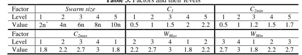
Since setting the parameters has an influence on the performance of the algorithms; in this paper, the Taguchi (1986) method, one of the most famous methods for the parameter selections, with five levels for each parameter is used. Table 3 shows these factors and their levels.
Table 3. Factors and their levels
Factor Swarm size C1 C2min
Level 1 2 3 4 5 1 2 3 4 5 1 2 3 4 5
Value 2n* 4n 6n 8n 10n 0.5 1 1.5 2 2.2 0.5 1 1.2 1.5 1.7
Factor C2max WMax WMin
Level 1 2 3 4 1 2 3 4 1 2 3 4 1 2 3
Value 1.8 2.2 2.7 3 1.8 2.2 2.7 3 1.8 2.2 2.7 3 1.8 2.2 2.7
In the Taguchi method, orthogonal arrays are used to decrease the number of experiments. These arrays are presented in table 4. It shows that 25 tests are necessary to select the best parameters.
Table 4. The orthogonal arrays for the proposed approach
Test 1 2 3 4 5 6 7 8 9 10 11 12 13 14 15 16 17 18 19 20 21 22 23 24 25
Swarm size 1 1 1 1 1 2 2 2 2 2 3 3 3 3 3 4 4 4 4 4 5 5 5 5 5
C1 1 2 3 4 5 1 2 3 4 5 1 2 3 4 5 1 2 3 4 5 1 2 3 4 5
C2min 1 2 3 4 5 2 3 4 5 1 3 4 5 1 2 4 5 1 2 3 5 1 2 3 4
C2max 1 2 3 4 5 3 4 5 1 2 5 1 2 3 4 2 3 4 5 1 4 5 1 2 3
Wmax 1 2 3 4 5 4 5 1 2 3 2 3 4 5 1 5 1 2 3 4 3 4 5 1 2
Wmin 1 2 3 4 5 5 1 2 3 4 4 5 1 2 3 3 4 5 1 2 2 3 4 5 1
Each test is run five times and the average of the objective function is obtained to calculate the (S/N) ratio. These values help to make a better decision. This ratio is given as follows:
𝑆𝑁 = −10 log(1
𝑛∑ (𝑜𝑏𝑗𝑒𝑐𝑡𝑖𝑣𝑒 𝑓𝑢𝑛𝑐𝑡𝑖𝑜𝑛)
2 𝑛
𝑖=1 ) (38)
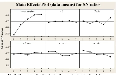
Fig 3. The mean SN ratio plot for the selected levels of each factor
According to figure 3, the maximum SN ratio shows the best level for each factor. The obtained results for parameter selections are presented in table 5.
Table 5. The parameters of PSO algorithm and their selected levels Factor Swarm
size
Cognitive coefficient (C1)
Minimum Social coefficient (C2min)
Maximum Social coefficient (C2max)
Maximum inertia weight (WMax)
Minimum inertia weight (WMin)
Level 5 4 5 4 2 1
value 10n 2 1.7 3 1 0.3
4-2- Numerical example
In this section, the proposed approach is illustrated by using a problem with nine tasks, two models and three levels of skills. The production planning horizon and the capacity of each station are 480 units of time. The required data for this example are shown in table 6.
Fig 4. The precedence diagram between the tasks
M e a n o f S N r a ti o s 5 4 3 2 1 6.4 6.2 6.0 5.8 5 4 3 2
1 1 2 3 4 5
5 4 3 2 1 6.4 6.2 6.0 5.8 5 4 3 2
1 1 2 3 4 5
swarm-size c1 c2min
c2max wmax wmin
Main Effects Plot (data means) for SN ratios
Table 6. Data of the example
Task Side Model A Model B
Skill 1 Skill 2 Skill 3 Skill 1 Skill 2 Skill 3
1 L 1 2 3 0 0 0
2 R 2 3 4 1 2 3
3 E 0 0 0 1 2 4
4 L 2 3 5 0 0 0
5 R 1 3 4 1 3 4
6 E 1 2 3 1 2 3
7 E 1 3 4 2 3 4
8 L 0 0 0 3 4 6
9 E 1 3 5 1 2 3
Human cost 900 600 400 900 600 400
Profit 50 90
Demand 100 40
According to the task times, production planning horizon and the demand of each model, the first cycle is 6. An initial worker assignment and line balancing are presented in table 7. It shows the assembly line has two mated-stations and four stations.
Table 7. Initial tasks and worker assignments to the mated-stations Mated-station 1 Mated-station 2
Left-side Right-side Left-side Right-side
Task 1, 4 2, 3 6, 7, 8 5, 9
Skill 1 2 1 2
The required time for each station according to table 7 is presented in table 8.
Table 8. Initial required time for each station and model Mated-station 1 Mated-station 2 Left-side Right-side Left-side Right-side
Skill 1 2 1 2
Required time1(A) 3 3 2 6
Required time1(B) 0 4 6 5
The required capacity for each station is shown in table 9. This table shows that if there are these workers in the stations and line balancing; the right side of the mated-station 2 will be a bottleneck.
Table 9. The initial required capacity for each station Mated-station 1 Mated-station 2 Left-side Right-side Left-side Right-side
Skill 1 2 1 2
Required capacity1(A) 300 300 200 600
Required capacity1(B) 0 160 240 200
Total required capacity1 300 460 440 800
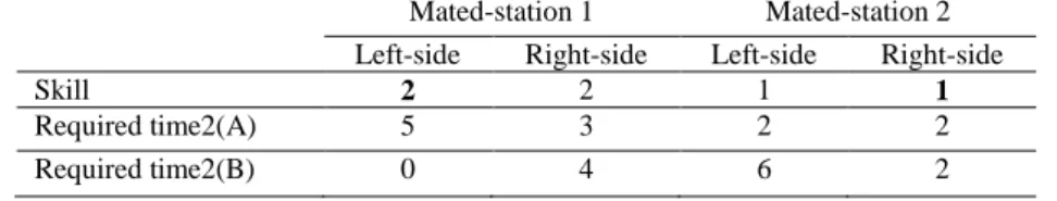
In this situation, it is tried to eliminate the bottleneck by interchanging the positions of the two operators on this line. Clearly, the bottleneck has a medium-skilled worker. However, the left-side of the mated-station 1 that is not a bottleneck has a high-skilled worker. Therefore, it is necessary to verify that if this change occurs, will the station time be lower than the cycle time or not? Table 10 and table 11 shows these results.
Table 10. The required time for each station and model after changing the positions of two operators Mated-station 1 Mated-station 2
Left-side Right-side Left-side Right-side
Skill 2 2 1 1
Required time2(A) 5 3 2 2
Table 11. The required capacity for each station after changing the positions of two operators Mated-station 1 Mated-station 2
Left-side Right-side Left-side Right-side
Skill 2 2 1 1
Required capacity2(A) 500 300 200 200
Required capacity2(B) 0 160 240 80
Total required capacity2 500 460 440 280
Table 11 shows that changing the position of the operators led to the reduction of the work overload of the line; however, the bottleneck was not eliminated. Thus, determining the 'R' index for product-mix is necessary:
𝑅𝐴= 50
5 = 10, 𝑅𝐵 = 90
0 = ∞
Since RB>RA, the first priority of the production is of model B. The product-mixes are QB=40 and
QA= [ 480
5 ] = 96.
Table 12. The required capacity for each station after product-mix determination
Mated-station 1 Mated-station 2
Left-side Right-side Left-side Right-side
Skill 2 2 1 1
Required capacity3(A) 480 288 192 192
Required capacity3(B) 0 160 240 80
Total required capacity 480 448 432 278
In this condition, the cycle time may change. As the result, it will be necessary to recalculate it. C=max{6, 480
96+40}=6
Since the cycle time does not change and there is no bottleneck, the algorithm should be stopped, and the objective functions can be calculated.
5- Computational results and discussion
In this section, alongside the proposed algorithm, another algorithm is developed based on the structure of the proposed algorithm. Simulated annealing and theory of constraints were used and it was called hybrid SA-TOC. The efficiencies of both algorithms are examined over a set of benchmarked test problems in terms of running time and solution quality.
In these problems, there are two product models and three skill levels (low, medium, and high) with $400, $600 and $900 human cost for each operator. The weights of the objective functions are W1=W2=W3=0.3 and W4=0.1. Furthermore, for better analysis, three demand levels are used for each
model. More details of the problems are shown in table 13.
Table 13. The number of tasks, demands and the profit of each model
Problem P 9D1 P 9D2 P 9D3 P 12D1 P 12D2 P 12D3 P 14D1 P 14D2 P 14D3 P 20D1 P 20D2 P 20D3 P 25D1 P 25D2 P 25D3 P 30D1 P 30D2 P 30D3 P 39D1 P 39D2 P 39D3 P 47D1 P 47D2 P 47D3 P 65D1 P 65D2 P 65D3
No.tasks 9 9 9
12 12 12 14 14 14 20 20 20 25 25 25 30 30 30 39 39 39 47 47 47 65 65 65
DA
100 40 70 90 45 65 70 30 50 70 30 50 38 10 24 70 30 50 60 30 45 20 8 14 70 30 50
DB
40 100 70 45 90 65 30 70 50 30 70 50 10 38 24 30 70 50 30 60 45 8 20 14 30 70 50
PrA
90 90 90 90 90 90 70 70 70 90 90 90 70 70 70 70 70 70 70 70 70 90 90 90 900 900 900
PrB
50 50 50 50 50 50 50 50 50 50 50 50 50 50 50 45 45 45 50 50 50 50 50 50 450 450 450
DP
480 480 480 480 480 480 480 480 480 960 960 960 960 960 960 960 960 960 960 960 960 800 800 800 23040 23040 23040
The algorithm is coded in MATLAB software and run on a personal computer with Intel (R) Core (TM) i3-2120 CPU @ 3.30 GHz and 4 GB of RAM memory. Each problem is solved four times.
Table 14 shows the results of using the proposed algorithms for the minimum, average and maximum WSI, THC and Z.
Table 14. Obtained results for WSI, THC and Z by hybrid PSO-TOC and hybrid SA-TOC algorithms
Problem WSI (hybrid SA-TOC) WSI (hybrid PSO-TOC) 0.01×THC (hybrid SA-TOC) 0.01×THC (hybrid PSO-TOC) 100×Z (hybrid SA-TOC) 100×Z (hybrid PSO-TOC)
M*** A** M* M A m M A m M A M M A m M A M
P9D1 0.71 0.18 0.00 2.00 0.50 0.00 18 15.75 15 15 15 15 48 41 38 28 27 25 P9D2 0.38 0.38 0.38 1.54 0.90 0.38 18 17.25 15 15 15 15 53 40 30 24 23 21 P9D3 3.76 1.32 0.50 1.50 1.30 0.71 21 18.75 18 18 15.75 15 66 56 50 26 25 23 P12D1 1.60 1.06 0.71 2.17 1.47 0.92 30 28.50 28 27 24.25 22 66 53 42 29 29 28 P12D2 1.73 1.27 0.86 2.43 1.89 1.61 33 29.25 26 22 72.75 22 89 59 45 29 29 27 P12D3 1.94 1.38 0.73 1.73 1.41 1.05 31 30.25 30 27 25.75 22 53 50 47 30 29 29 P14D1 5.50 3.41 2.02 2.83 2.39 1.58 46 43.25 39 41 38.75 37 60 58 56 46 46 44 P14D2 5.32 3.98 2.69 6.56 5.23 3.54 47 45.75 44 43 40.50 37 75 72 57 45 44 43 P14D3 4.60 3.23 2.02 4.96 3.02 1.37 49 45.00 42 42 39.25 37 74 66 56 47 46 45 P20D1 6.98 5.93 4.38 4.42 3.13 2.27 59 56.50 54 51 49.50 48 79 72 61 52 50 47 P20D2 5.23 4.57 3.98 8.25 6.69 6.12 61 58.00 53 55 53.25 52 79 74 72 51 50 49 P20D3 5.75 4.81 3.45 6.32 4.92 3.82 62 58.25 56 54 53.00 52 85 76 68 51 50 48 P25D1 10.53 10.23 10.05 19.3 18.5 17.6 93 89.75 87 81 79.25 77 91 85 76 63 62 62 P25D2 14.83 12.27 10.68 10.8 10.64 10.56 92 83.75 80 84 79.50 75 85 80 77 60 59 57 P25D3 14.32 11.73 10.50 14.88 14.85 14.80 90 83.00 79 79 77.25 75 79 76 72 63 61 60 P30D1 6.01 5.52 4.57 5.05 4.56 4.05 82 80.75 78 75 71.50 64 87 82 74 57 55 55 P30D2 6.90 5.28 4.33 4.72 4.23 3.78 83 79.50 77 82 77.50 72 82 77 74 57 56 56 P30D3 6.10 5.64 5.11 5.76 5.36 4.96 88 83.25 79 76 73.25 72 91 80 64 57 56 56 P39D1 8.27 7.76 7.54 9.98 8.68 6.48 93 90.50 87 91 85.00 79 92 80 70 55 54 52 P39D2 7.29 6.62 5.50 10.64 9.55 8.62 97 90.25 80 93 84.50 78 95 82 76 57 55 54 P39D3 7.36 7.29 7.22 10.67 10.17 9.24 93 87.75 81 85 81.50 77 85 78 74 56 55 54 P47D1 16.56 15.22 14.20 28.16 26.20 24.82 120 109 102 101 98.3 96 97 86 78 61 60 59 P47D2 18.22 16.59 14.93 30.87 28.69 26.56 109 104 99 108 101.8 95 86 81 76 61 61 60 P47D3 19.82 17.67 15.69 29.87 28.19 27.26 114 102 96 107 98.75 88 89 85 73 62 62 61 P65D1 124.90 106.07 78.20 127.1 106.8 83.62 84 79.75 78 71 69.50 67 79 74 67 53 52 52 P65D2 123.76 108.48 102.68 161.3 134.8 115.0 87 83 79 79 67.25 57 93 81 73 53 53 51 P65D3 124.01 116.97 108.53 140.1 120.7 101.1 90 83.25 77 72 70. 68 91 84 75 54 53 53
m*: minimum; A**: average; M***: maximum
Table 15 presents the obtained product-mix and the total profit of the both algorithms.
Table 15. The obtained results for the product-mix and the total profit
Problem Product-mix(hybrid SA-TOC) Product-mix(hybrid PSO-TOC) TP(hybrid SA-TOC) TP(hybrid PSO-TOC)
A(m,Ave,M) B(m,Ave,M) A(m,Ave,M) B(m,Ave,M) M*** Ave** M* M Ave M
P9D1 (80, 84, 96) (0, 0, 0) (80, 80, 80) (0, 0, 0) 8640 7560 7200 7200 7200 7200 P9D2 (40, 40, 40) (40, 52, 56) (40, 40, 40) (40, 40, 40) 7200 6200 5600 5600 5600 5600 P9D3 (70, 70, 70) (12, 22.5, 26) (70, 70, 70) (10, 12.75, 21) 7600 7425 6900 7350 6937.5 6800 P12D1 (90, 90, 90) (10, 23, 36) (90, 90, 90) (10, 15.25, 31) 9900 9250 8600 9650 8862.5 8600 P12D2 (45, 45, 45) (61, 68.25, 80) (45, 45, 45) (55, 57.75, 66) 8850 7462.5 7100 7350 6937.5 6800 P12D3 (65, 65, 65) (37, 47.5, 65) (65, 65, 65) (35, 45.5, 54) 9100 8225 7700 8550 8125 7600 P14D1 (50,51.5, 53) (0, 0, 0) (50, 50, 50) (0, 0, 0) 3710 3605 3500 3500 3500 3500 P14D2 (30, 30, 30) (20, 26.5, 30) (30, 30, 30) (20, 22.5, 24) 3600 3425 3100 3300 3225 3100 P14D3 (50, 50, 50) (0, 2.25, 6) (50, 50, 50) (0, 0.75, 3) 3800 3612.5 3500 3650 3537.5 3500 P20D1 (68, 69, 70) (0, 1.75, 4) (68, 68, 68) (0, 0, 0) 6500 6297.5 6120 6120 6120 6120 P20D2 (30, 30, 30) (40, 46.5, 60) (30, 30, 30) (38, 39.5, 40) 6500 5025 4700 4700 4675 4600 P20D3 (50, 50, 50) (23, 31.25, 36) (50, 50, 50)s (22, 22, 22) 6300 6062.5 5650 5600 5600 5600 P25D1 (35,36.75,38) (2, 6.25, 10) (34,36.25,38) (4, 7.25, 10) 2950 2885 2760 2950 2900 2860 P25D2 (10, 10, 10) (31, 35.25, 38) (10, 10, 10) (31, 32.5, 34) 2950 2462.5 2250 2400 2325 2250 P25D3 (24, 24, 24) (16, 22, 24) (24, 24, 24) (16, 19, 21) 2880 2735 2400 2730 2630 2480 P30D1 (68,69.5,70) (1, 3.75, 5) (68, 68, 68) (0, 0, 0) 5125 4988.75 4805 4760 4760 4760 P30D2 (30, 30, 30) (40, 43.25, 46) (30, 30, 30) (38, 39.5, 41) 5125 4046.25 3900 3945 3877.5 3810 P30D3 (50, 50, 50) (18, 21.75, 25) (50, 50, 50) (18, 18.5, 20) 4625 4433.8 4130 4400 4332.5 4310 P39D1 (60, 60, 60) (4, 7, 12) (60, 60, 60) (4, 5, 8) 4800 4550 4400 4600 4450 4400 P39D2 (30, 30, 30) (34, 37.5, 40) (30, 30, 30) (34, 37.5, 40) 4400 3975 3800 4100 3975 3800 P39D3 (45, 45, 45) (19, 21.5, 23) (45, 45, 45) (19, 19, 19) 4300 4225 4100 4100 4100 4100 P47D1 (20, 20, 20) (3, 3.75, 4) (20, 20, 20) (3, 4.5, 5) 2000 1962.5 1950 2050 2025 1950 P47D2 (8, 8, 8) (17, 17.5, 19) (8, 8, 8) (15, 15.5, 16) 1950 1595 1570 1520 1495 1470 P47D3 (14, 14, 14) (9, 10.25, 11) (14, 14, 14) (10, 10.75, 11) 1810 1772.5 1710 1810 1797.5 1760 P65D1 (70, 70, 70) (18, 23, 25) (70, 70, 70) (22, 23.25, 25) 74250 73350 71100 74250 73462.5 72900 P65D2 (30, 30, 30) (60, 65.25, 70) (30, 30, 30) (59, 63, 66) 73800 56362.5 54000 56700 55350 53550 P65D3 (50, 50, 50) (41, 45.25, 50) (50, 50, 50) (43, 44.5, 46) 67500 65362.5 63450 65701 65025.25 64350
m*: minimum; Ave**: average; M***: maximum; A: model A; B: Model B
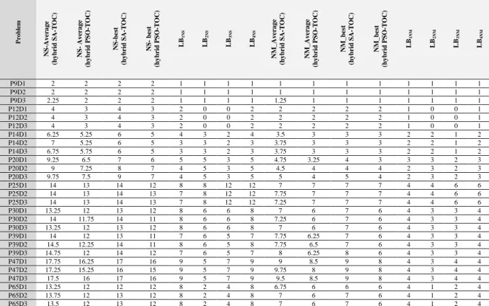
Table 16 displays the lower bounds, the average and the best numbers of the stations and the mated-stations which are obtained using the hybrid PSO-TOC and the hybrid SA-TOC.
Table 16. The lower bounds and the number of stations and the number of mated-stations by the both algorithms P rob lem NS -Average (hybrid SA -TOC) NS - Average (hybrid PSO -TOC) NS -best (hybrid SA -TOC) NS - best (hybrid PSO -TOC) LB 1 N S LB 2 N S LB 3 N S LB 4 N S NM_Average (hybrid SA -TOC) NM_Average (hybrid PSO -TOC) NM_best (hybrid SA -TOC) NM_best (hybrid PSO -TOC) LB 1 N M LB 2 N M LB 3 N M LB 4 N M
P9D1 2 2 2 2 1 1 1 1 1 1 1 1 1 1 1 1
P9D2 2 2 2 2 1 1 1 1 1 1 1 1 1 1 1 1
P9D3 2.25 2 2 2 1 1 1 1 1.25 1 1 1 1 1 1 1
P12D1 4 3 4 3 2 0 0 2 2 2 2 2 1 0 0 1
P12D2 4 3 4 3 2 0 0 2 2 2 2 2 1 0 0 1
P12D3 4 3 4 3 2 0 0 2 2 2 2 2 1 0 0 1
P14D1 6.25 5.25 6 5 4 3 2 4 3.5 3 3 3 2 2 1 2
P14D2 7 5.25 6 5 3 3 2 3 3.75 3 3 3 2 2 1 2
P14D3 6.75 5.75 6 5 3 3 2 3 3.75 3 3 3 2 2 1 2
P20D1 9.25 6.5 7 6 5 5 3 5 4.75 3.25 4 3 3 3 2 3
P20D2 9 7.25 8 7 4 5 3 5 4.5 4 4 4 2 3 2 3
P20D3 9.75 7.5 9 7 4 5 3 5 5 4 5 4 2 3 2 3
P25D1 14 13 14 12 8 8 12 12 7 7 7 7 4 4 6 6
P25D2 14 13 14 13 7 8 12 12 7.75 7 7 7 4 4 6 6
P25D3 14 13 14 13 7 8 12 12 7.25 7 7 7 4 4 6 6
P30D1 13.25 12 13 12 8 6 6 8 7 6 7 6 4 3 3 4
P30D2 14 11.75 14 11 8 6 6 8 7.25 6 7 6 4 3 3 4
P30D3 13.25 12 13 12 8 6 6 8 7 6 7 6 4 3 3 4
P39D1 14 12 13 11 7 6 5 7 7.75 6.25 7 6 4 3 3 4
P39D2 14.5 12.25 14 11 8 6 5 8 7.75 6.5 7 6 4 3 3 4
P39D3 14.75 12 14 12 7 6 5 7 8 6.25 8 6 4 3 3 4
P47D1 17.75 16.25 17 16 9 5 7 9 9 8.5 9 8 4 3 4 4
P47D2 17.25 15.25 16 15 9 5 7 9 9.75 8 9 8 4 3 4 4
P47D3 17.5 16 17 16 9 5 7 9 9.5 8.5 9 8 4 3 4 4
P65D1 13.25 12 12 12 8 2 4 8 6.75 6 6 6 4 1 2 4
P65D2 13.75 12 13 12 8 2 4 8 7 6 7 6 4 1 2 4
P65D3 13.5 12 13 12 8 2 4 8 7 6 7 6 4 1 2 4
Figure 5 and figure 6 show the differences between the obtained results from the number of the stations, the number of the mated-stations and the best lower bound. They demonstrate that the hybrid PSO-TOC has better results for the number of the mated-stations and the number of the stations. It means that by using this algorithm a shorter line is obtained. In addition, these figures show that the differences between both algorithms and the lower bound for small-sized problems are negligible. Moreover, the difference between the obtained results utilizing the hybrid PSO-TOC and the lower bound is small.
Fig 5. Comparison between the obtained results for the number of mated-stations by hybrid PSO-TOC, hybrid SA-TOC and lower bound
Fig 6. Comparison between the obtained results for the number of stations by hybrid PSO-TOC, hybrid SA-TOC and best lower bound
One of the most significant decisions in stage 1 of the proposed algorithm is the value of each skill worker’s determination. The obtained results for the minimum, the average and the maximum number of each skilled worker are illustrated in table 17.
Table 17. Minimum (m), average (Ave) and maximum (M) numbers of each skill for both algorithms
Problem
Skill1 (hybrid SA-TOC)
Skill1 (hybrid PSO-TOC)
Skill2 (hybrid SA-TOC)
Skill2 (hybrid PSO-TOC)
Skill3 (hybrid SA-TOC)
Skill3 (hybrid PSO-TOC)
m Ave M M Ave M m Ave M m Ave M m Ave M m Ave M
P9D1 1 1.25 2 0 0 0 0 0.75 1 0 0 0 0 0 0 0 0 0
P9D2 1 1.75 2 1 1 1 0 0.25 1 1 1 1 0 0 0 0 0 0
P9D3 1 1.75 2 1 1.25 2 0 0.5 2 0 0.75 1 0 0 0 0 0 0
P12D1 2 2 2 2 2.75 3 1 1.25 2 0 0.5 1 0 0.75 1 0 0.25 1
P12D2 2 2.25 3 2 2.75 3 0 1 2 0 0 0 0 0.75 2 0 0.75 1
P12D3 2 2.25 3 2 2.75 3 1 1.5 2 0 0 0 0 0.25 1 0 0.25 1
P14D1 1 2.75 4 3 3.75 4 1 2.25 3 0 0.75 1 0 1.25 3 1 1.25 2
P14D2 0 2.25 3 3 3.5 4 2 4.25 6 0 1 2 0 1.5 2 0 0.75 1
P14D3 3 4.5 6 2 2.75 3 0 1 2 1 2.5 4 0 0.75 1 0 1 2
P20D1 1 2.5 5 2 4 5 1 3.25 6 1 1.75 3 1 3 7 0 0.75 3
P20D2 1 2.5 3 3 3.5 5 3 4.75 8 0 1.5 3 0 1.75 4 1 1.5 2
P20D3 2 4.25 5 3 3.5 4 3 6.25 11 2 2.75 3 1 3.5 6 0 1.25 2
P25D1 2 4.25 5 2 3.25 5 3 6.25 11 2 5.5 7 1 3.5 6 3 4.25 5
P25D2 2 2.75 4 3 3.5 4 5 7 8 5 6 7 2 4.25 6 3 3.5 5
P25D3 1 2.5 4 1 2.25 3 5 7.25 9 6 7 9 3 4.25 6 3 3.75 4
P30D1 2 3.25 4 2 2.5 3 5 5.75 7 3 5.5 7 3 4.25 6 3 4 7
P30D2 1 2 3 2 3.5 6 6 6.75 8 1 5.75 9 5 5.25 6 0 2.5 4
P30D3 2 4 6 3 3.5 4 3 4.75 7 2 4.25 6 4 4.75 6 3 4.25 6
P39D1 3 4.5 7 5 5.5 7 1 6 8 4 4.75 5 1 3.5 6 1 1.75 3
P39D2 2 3.75 6 3 5 7 5 6.75 9 2 5.25 8 3 4 5 0 2 4
P39D3 1 3.75 4 3 4 5 5 7.5 11 6 6.75 8 3 4.5 6 0 1.25 2
P47D1 4 5 6 2 3.25 5 5 6.5 9 6 8.5 11 3 6.25 9 3 4.5 7
P47D2 3 3 3 3 5.25 6 8 10 11 5 7.25 9 3 4.25 7 0 2.75 5
P47D3 1 2 4 2 3.75 5 9 11 14 6 8 10 2 4.5 7 2 4.25 7
P65D1 0 2.25 4 1 2.5 3 6 7.75 11 3 4.5 7 1 3.25 6 4 5 6
P65D2 2 3.75 5 1 1.75 3 3 5.25 9 2 5.25 8 3 5 7 1 4 9
P65D3 1 2.25 4 2 2 2 7 9 10 5 6 7 1 2.25 3 3 4 5
Figure 7 shows the obtained results of the best human costs of the hybrid PSO-TOC and the hybrid SA-TOC. This figure indicates that the results of the hybrid PSO-TOC are better than the results of the hybrid SA-TOC. It means that in addition to impacting the number of stations and the number of the mated-stations, the hybrid PSO-TOC algorithm produces better results for human costs.
Fig 7. Comparison between the obtained results for total human cost by hybrid PSO-TOC and hybrid SA-TOC
Figure 8 compares the obtained weighted smoothness indexes of both algorithms. It shows that in most of the cases the result of WSI of the hybrid SA-TOC is better than the WSI of the hybrid PSO-TOC.
Fig 8. Comparison between the best obtained results for WSI by hybrid PSO-TOC and hybrid SA-TOC
Figure 9 presents the obtained 'Z' for both algorithms and indicates that the results of the hybrid PSO-TOC are better than the hybrid SA-TOC.
Fig 9. Comparison between the best obtained results for 'Z' by hybrid PSO-TOC and hybrid SA-TOC
The only objective function of stage 2 is total profit maximization and product-mix determination using the theory of constraints. Figure 10 shows that hybrid SA-TOC has better total profit than the hybrid PSO-TOC algorithm.
Fig 10. Comparison between the total profit by hybrid PSO-TOC and hybrid SA-TOC
In addition to the above figures, two comparisons between both algorithms are presented for the average number of iterations and the elapsed time to obtain the Z-best in figure 11 and figure 12.
Fig 11. Comparison between the average number of iterations to obtain the best results of 'Z' by hybrid PSO-TOC and hybrid SA-PSO-TOC
Figure 11 shows that there is no discipline for the number of iterations to achieve the best results from worker assignment and line balancing.
Fig 12. Comparison between the elapsed time to obtain the best results of 'Z' by hybrid PSO-TOC and hybrid SA-TOC
Figure 12 demonstrates that the hybrid SA-TOC is faster than the hybrid PSO-TOC. However, the differences between the elapsed times for the small-sized problems are negligible.
Figure 13 presents the percentage of the stations which were bottlenecks (Bottleneck %) in the last part of stage 1. It shows that the values of the small-sized problems for the hybrid PSO-TOC are more than the results of the hybrid SA-TOC and large-sized problems.
Fig 13. The average of Bottleneck% for the both algorithms
6- Conclusion
This paper dealt with a multi-objective mixed-model TSALBP with worker assignment and bottleneck analysis when the task times are dependent on the worker’s skill. The considered objective functions were Minimizing the number of mated-stations, the number of stations, the human costs, the weighted smoothness index and maximizing the total profit.
To solve the mentioned problem, a cyclic-hierarchical algorithm (hybrid PSO-TOC) was presented and another algorithm based on the structure of the proposed algorithm was developed (hybrid SA-TOC). In addition, several problems with different conditions were tested using the proposed approach.
These algorithms had two stages. In stage one, worker assignment and line balancing were done simultaneously. In stage two, eliminating the bottlenecks and product-mix determination were considered. Additionally, several lower bounds were developed for the number of stations and the number of mated-stations. The obtained results indicated that the hybrid PSO-TOC has fewer numbers of mated-stations, stations and human costs than the hybrid SA-TOC. However, the hybrid SA-TOC showed better results for the total profit, the product-mix determination and the elapsed time. Alongside using the other methods to solve the problem, this research can be enriched with other assumptions, such as the learning effect, the U-shaped lines and the parallel stations for future research.
References
Araújo, F.B., Costa, A, M., & Miralles, C. (2012). Two extensions for the ALWABP: Parallel stations and collaborative approach. International Journal of Production Economics, 140, 483–495.
Bartholdi, J.J. (1993). Balancing two-sided assembly lines: a case study. International Journal of Production Research, 31(10), 2447–2461.
Battaïa, O., & Dolgui, A. (2013). A taxonomy of line balancing problems and their solution approaches. International Journal of Production Economics, 142(2), 259–277.
Blum, C., & Miralles, C. (2011). On solving the assembly line worker assignment and balancing problem via beam search. Computers & Operations Research, 38, 328–339.
Worker Assignment and Balancing Problem. Computers & Operations Research 4587–4596.
Boysen, N., Fliedner, M., & Scholl, A. (2007). A classification of assembly line balancing problems. European Journal of Operational Research, 183, 674–693.
Boysen, N., Fliedner, M., & Scholl, A. (2008). Assembly line balancing: Which model to use when?. International Journal of Production Economics, 111, 509–528.
Chutima, P., & Chimklai, P. (2012). Multi-objective two-sided mixed-model assembly line balancing using particle swarm optimisation with negative knowledge. Computers and Industrial Engineering, 62, 39–55.
Costa, A. M., & Miralles, C. (2009). Job rotation in assembly lines employing disabled workers. International Journal of Production Economics, 120, 625–632.
Deb, K. (2001). Multi-Objective Optimization Using Evolutionary Algorithms. John Wiley and Sons, Inc, New York, NY, USA.
Hamta, N., Fatemi Ghomi, S.M.T., Jolai, F., & Akbarpour Shirazi, M. (2013). A hybrid PSO algorithm for a multi-objective assembly line balancing problem with flexible operation times, sequence-dependent setup times and learning effect. International Journal of Production Economics, 141(1), 99-111.
Hu, S.J., Ko, J., Weyand, L., El Maraghy, H.A., Lien, T.K., Koren, Y., Bley, H., Chryssolouris, G., Nasr, N., & Shpitalni, M. (2011). Assembly system design and operations for product variety. CIRP Annals-Manufacturing Technology, 60, 715–733.
Kennedy, J., & Eberhart, R.C. (1995). Particle swarm optimization. In proceedings of IEEE international Conference on Neural Networks (Perth, Australia). 1942-1948.
Miralles, C., García-Sabater, J. P., Andrés, C., & Cardos, M. (2007). Advantages of assembly lines in Sheltered Work Centres for Disabled. A case study. International Journal of Production Economics, 110, 187–197.
Miralles, C., Garía-Sabater, J. P., Andrés, C., & Cardós, M. (2008). Branch and bound procedures for solving the Assembly Line Worker Assignment and Balancing Problem: Application to Sheltered Work centres for Disabled. Discrete Applied Mathematics, 156, 352-367.
Moreira, M. C. O., Ritt, M., Costa, A. M., & Chaves, A. A. (2012). "Simple heuristics for the assembly line worker assignment and balancing problem. Journal of Heuristics, 18, 505–524.
Mutlu, Ö., Polat, O., & Supciller, A. A. (2013). An iterative genetic algorithm for the assembly line worker assignment and balancing problem of type-II. Computers & Operations Research, 40 (1), 418– 426.
Özcan, U., & Toklu, B. (2009). Balancing of mixed-model two-sided assembly lines. Computers and Industrial Engineering, 57, 217–227.
Özcan, U., Gokcen, H., & Toklu, B. (2010). Balancing parallel two-sided assembly lines. International Journal of Production Research, 48 (16), 4767–4784.
Pastor, R. (2011). LB-ALBP: the lexicographic bottleneck assembly line balancing problem. International Journal of Production Research, 49(8), 2425-2442.
Pastor, R., Chueca, I., & García-Villoria, A. (2012). A heuristic procedure for solving the Lexicographic Bottleneck Assembly Line Balancing Problem (LB-ALBP). International Journal of Production Research, 50(7), 1862-1876.
Purnomo, H. D., Wee, H. M., & Rau, H. (2013). Two-sided assembly lines balancing with assignment restriction. Mathematical and Computer Modeling, 57, 189–199.
Salveson, M.E. (1955). The assembly line balancing problem. Journal of Industrial Engineering, 6(3), 18–25.
Scholl, A. (1999). balancing and sequencing of assembly lines. Physica-Verlag.
Scholl, A., & Becker, C. (2006). State-of-the-art exact and heuristic solution procedures for simple assembly line balancing. European Journal of Operational Research, 168, 666–693.
Simaria, A. S., & Vilarinho, P. M. (2009). 2-ANTBAL: An ant colony optimization algorithm for balancing two-sided assembly lines. Computers & Industrial Engineering, 56, 489–506.
Sirovetnukul, R., & Chutima, P. (2010). The Impact of Walking Time On U-Shaped Assembly Line Worker Allocation Problems. Engineering Journal, 14 (2), 53-78.
Song, B.L., Wong, W.K., Fan, J.T., & Chan, S.F. (2006). A recursive operator allocation approach for assembly line balancing optimization problem with the consideration of operator efficiency. Computers & Industrial Engineering, 51, 585–608.
Taguchi, G. (1986). Introduction to Quality Engineering. Asian Productivity organization.
Vilà, M., & Pereira, J. (2014). A branch-and-bound algorithm for assembly line worker assignment and balancing problems. Computers & Operations Research, 44, 105–114.
Xiaofeng, H., Erfei, W., Jinsong, B., & Ye, J. (2010). A branch-and-bound algorithm to minimize the line length of a two-sided assembly line. European Journal of Operational Research, 206, 703–707. Zaman, T., Paul, S. K., & Azeem, A. (2012). Sustainable operator assignment in an assembly line using genetic algorithm. International Journal of Production Research, 50 (18), 5077–5084.
Zhang, W., Gen, M., Lin, L. (2008). A Multi-objective Genetic Algorithm for Assembly Line Balancing Problem with Worker Allocation, IEEE International Conference on Systems, Man and Cybernetics.