An Optimal Radial Basis Function (RBF) Neural
Network for Hyper-Surface Reconstruction
A. Shahsavand
1Abstract. Data acquisition of chemical engineering processes is expensive and the collected data are always contaminated with inevitable measurement errors. Ecient algorithms are required to lter out the noise and capture the true underlying trend hidden in the training data sets. Regularization networks, which are the exact solution of multivariate linear regularization problems, provide an appropriate means to perform such a demanding task. These networks can be represented as a single hidden layer neural network with one neuron for each distinct exemplar. Ecient training of a regularization network requires the calculation of linear synaptic weights, selection of isotropic spread () and computation of an optimum level of regularization (). The latter parameters ( and ) are highly correlated with each other. A
novel method is presented in this article for the development of a convenient procedure for de-correlating the above parameters and selecting the optimal values of and . The plot of versus suggests
a threshold that can be regarded as the optimal isotropic spread for which the regularization network
provides appropriate model for the training data set. It is also shown that the eective degrees of freedom of a regularization network is a function of both regularization levels and isotropic spread. A readily calculable measure of the approximate degrees of freedom of a regularization network is also introduced, which may be used to de-couple and .
Keywords: Neural network; Regularization network; Function approximation; Optimum spread; Degrees of freedom.
INTRODUCTION
Despite the tremendous increase in application of neural networks in many elds, such as electrical, electronics, civil, and control engineering, they were practically unknown to many chemical engineers until the 1990's. Serious eorts to apply neural networks to the simulation and optimization of chemical, biochem-ical and mineral processes have only begun since the late 1980's [1-3].
Articial neural networks are usually classied as recurrent and feed-forward. The former networks are mostly used for the empirical modeling of control problems and the latter are well suited for classication or function approximations. The close relationship between the function approximation problem and feed-forward articial neural networks was explored
ear-1. Department of Chemical Engineering, Ferdowsi University of Mashhad, Mashhad, P.O. Box 91775-1111, Iran. E-mail: [email protected]
Received 17 March 2007; received in revised form 8 December 2007; accepted 1 July 2008
lier [4]. Within this framework, neural networks may be viewed as approximation techniques for reconstructing input-output mappings in high-dimensional spaces [5]. In neural network parlance, training (learning) is equiv-alent to nding a hyper-surface in a multidimensional space that provides the best t for the training data and generalization is equivalent to the use of this hyper-surface to interpolate within the domain of data where there are no examples [6].
Kernel based neural networks such as Radial Basis Function Networks (RBFNs) have been shown to possess good approximation capabilities. Poggio and Girosi [7,8] reported that among all feed-forward networks, RBFN enjoy the best approximation prop-erty [6]. Hunt et al. [9] presented further theoretical support for RBF networks.
The training of RBF networks with specied non-linearities (centers and spreads) reduces to an over-determined set of linear equations, which can be solved by a variety of highly stable techniques such as SVD (Singular Value Decomposition) or Kalman ltering [10]. These networks have a close connection
with the well studied subject of multivariate function approximation and enjoy a rm theoretical foundation. Due to the complexity of chemical engineering processes, the acquired data are always contaminated with heavy measurement errors. As a result, the employment of advanced noise ltering techniques is crucial to avoid over-tting (or tting the noise) phe-nomena [11]. RBF networks that have originated from a multivariate regularization theory can distinguish and lter-out the noise. These networks are ideal for capturing the true underlying trend from a set of heavily contaminated chemical engineering data.
It was shown [7,8] that the solution of the multi-variate regularization problem can be represented as a single hidden layer network, known as the regulariza-tion network. Regularizaregulariza-tion networks are tradiregulariza-tionally constructed using isotropic Gaussian basis functions. An illustrative example is employed to investigate the eect of the regularization level and the value of the isotropic spread, , on the performance of a regularization network. A convenient procedure is introduced for selecting the appropriate value of the isotropic spread, . To the best of our knowledge, this approach has not been addressed previously and makes a signicant improvement in the performance of the regularization networks.
STRICT INTERPOLATION PROBLEM We start by considering the strict interpolation prob-lem and the remarkable theorem due to Michelli [12], which pinpoints the importance of radial basis func-tions in multivariate function approximation and neu-ral networks. The strict interpolation problem may be stated as: \Given a set of N input s (xi 2 <P; i = 1; ; N), and the corresponding outputs, (yi,
i = 1:; ; N), nd a continuous multivariate function F (x) which maps the inputs to the output and satises the following N interpolating conditions":
F (xi) = yi; i = 1; ; N: (1)
Let us expand F (x) as a linear summation of N radial basis functions, each centered at a distinct data point:
F (x) =
N
X
j=1
wjj k x xj k
: (2)
Here j(r) represents a radial function whose argument
is a measure of the (Euclidean) distance from the known centre located at xj, r = k x xj k and the wj's are the weighting coecients. Equations 1 and 2
can be combined and stated in the compact form:
F = w; (3)
where F = [F (x1); F (x2); ; F (xN)]T, w = [w1; ; wN]T and is the NN interpolation matrix
with elements,
ij= xi xj: (4)
The theorem originally proved by Michelli [12] for multiquadrics basis functions states that: \if x1; x2; ; xN are N distinct points in <P, the
in-terpolation matrix, , is non-singular". All that is required is for the input vectors to be distinct and the elements of the interpolation matrix to be based on radial functions centered on the known distinct data points. In exact or innite precision arithmetic, the system in Equation 3 can always be solved to obtain the unique optimal weights:
w= 1y: (5)
The continuous function in Equation 2 with the optimal weights will satisfy the N interpolating conditions (Equation 1) exactly. It should be pointed out here that in practice we always deal with nite rather than innite precision arithmetic and as a result, the inter-polation matrix, , may turn out to be numerically singular. This does not violate Michelli's theorem; it only tells us that we must use higher precision for our calculations. The strict interpolation problem always has a solution in terms of radial basis functions centered at the data points, irrespective of the size of the data set N or the dimensions of the input vector, x.
A large class of RBFs are covered by the Michelli theorem [6,13,14]. The functions shown in Table 1 are of particular interest in the study of multivariate regularization and its implementation as RBF net-works. Michelli has proved that for localized basis functions such as Gaussian and Inverse Multiquadric, the interpolation matrix, , is positive denite. The Multiquadric and Thin Plate Spline functions are global and for these basis functions, the interpolation
Table 1. Various radial basis functions. Radial Basis Functions Formula
Gaussian (x; t; ) = exp( kx tk2 2 )
Multiquadrics (x; t; ) = [kx tk2+ 2]1 2
Inverse multiquadrics (x; t; ) = 1 [kx tk2+2]12
Thin plate splines (x; t; ) =hkx tk
i2n
lnkx tk
matrix is indenite with N 1 negative and one positive eigenvalues [6]. In principle, global radial basis functions construct a smoother t and local RBFs can extract more specialized features due to their locality. REGULARIZATION NETWORK WITH ISOTROPIC SPREADS
In a dierent approach, Poggio and Girosi [7,8] illus-trated that the solution of a multivariate regularization problem can be represented as:
(G + IN)w= y; (6)
where G is the N N symmetric Green's matrix with elements Gij = G(xi; xj) and is the regularization
parameter. In practice, we may always choose suciently large to ensure that the matrix (G + IN)
is positive denite and, hence, invertible. Equation 6 can be symbolized as the network shown in Figure 1. The network consists of a single hidden layer with N neurons and the activation function of the jth hidden neuron is a Green function, G(x; xj), centered at a particular data point, xj. The inuence of the regularization parameter, , is embedded in the unknown synaptic weights, w0
js.
Poggio and Girrosi [7,8] also pointed out that for a special choice of stabilizing operator, Green's function reduces to a multidimensional factorizable isotropic Gaussian basis function, which is both translationally and rotationally invariant, having an innite number of continuous derivatives [6].
G(x; xj) = exp" x xj
2 22 j # = p Y k=1 exp "
(xk xj;k)2
22 j
#
: (7)
The j appearing in Equation 7 denotes the isotropic
spread of the jth Green function, which is assumed identical for all input dimensions. The performance of
Figure 1. The regularization network.
the regularization network strongly depends on both the appropriate choice of the isotropic spread and the proper level of regularization [15]. The leave-one-out cross validation criterion [16] is used for ecient computation of the optimum regularization parameter, , for a given .
CV () = 1 N N X k=1 " eT
k(IN H())y
eT
k(IN H())ek
#2
; (8)
where N is the number of both the training exemplars and neurons of the regularization network, ek is the kth unit vector of size N, IN is the N N unit matrix
and H() is the smoother matrix originally dened by Hastie and Tibshirani [17]. (If we focus on the t at the observed data points x1; x2; ; xN a linear smoother
can be written as f = Sy where S = fSi;jg is an N N
smoother matrix [17].)
It is already known that, by denition, the regu-larization network is a linear smoother as developed by Poggio & Girrosi [7,8]. The generalization performance of such a network can be simply computed from f = Gw. Replacing w from Equation 6 results in:
f = G(G + I) 1y: (9)
Therefore, by denition of the smoother matrix, H() for the regularization network can be computed from:
H() = S = G(G + I) 1: (10)
The eective number of parameters or degrees of freedom (df) of a linear smoother is dened as the trace of the smoother matrix that is equal to the sum of its eigenvalues, df = tr(H()) (or sum of its diagonal elements). Evidently, the number of degrees of freedom is a function of the span and the predictor values in the data set; it is not a function of the response (y) [17].
The evaluation of H() and hence CV (), at each trial value of , requires the inversion of the N N matrix (G + I) and may prove too time-consuming. This can be avoided by resorting to the similarity transformation technique [4]. The basic idea was initially presented by Golub et al. [18] for ridge regression.
Equations 7 to 9 show that CV () is a complex function of both and . Therefore, the optimal value of the regularization parameter, (which minimizes
CV ()), is highly correlated with the value of the isotropic spread, . In other words, the appropri-ate value of greatly depends on for a specic
data set with a xed level of noise. The strong correlation between these two parameters ( and )
is extremely complicated and may not be described directly in analytical form. A simple indirect procedure is proposed in this article for the decoupling of such
powerful dependency and for nding the optimum value of spread and the corresponding optimal level of regularization for the given noisy data set. The motivation behind such a decoupling procedure is to train the best optimal network for reconstructing the true hyper-surface embedded in the bunch of a noisy data set. It is clearly shown that such an optimum trained network can successfully lter out the noise and provide the nest generalization performance.
An illustrative example presented in the next section demonstrates the strong correlation between and . A signicant contribution of this article
is the development of a convenient procedure for de-correlating these parameters and selecting the optimal values of and for the specied data set.
AN ILLUSTRATIVE EXAMPLE
To illustrate the capabilities and probable shortcom-ings of the regularization network, a three-dimensional (bivariate) synthetic example is presented in this sec-tion. The main reason for the selection of a 3D case study is its perfect visualization feature. Two-dimensional examples are too simple to mimic the real world and 4D+ case studies are hard to visualize.
The following function describes the true underlying relationship between two input variables (0 x1; x2
1 radians) and one response (output) variable, as shown in Figure 2.
Z =100(Sin(5:5x)Cos(3y))2+ 0:15
exp " x 0:5 0:4 2# exp " y 0:5 0:3 2# : (11) Since all experimental data are inevitably associated with some measurement errors (noise), the training
Figure 2. 3D plot of the bivariate example.
exemplars generated from the above surface are con-taminated with the random noise of uniform distribu-tion and known width in the following examples. The random vectors with zero mean and identity covariance matrices were generated using MATLAB software. To produce such random vectors, the following procedure may be employed: Suppose that a random vector, X, has a covariance matrix, Q. Since this matrix is Hermitian symmetric and positive semidenite, by the spectral theorem from linear algebra, we can diagonalize or factor the matrix in the following way:
Q = EET; (12)
where E is the orthogonal matrix of eigenvectors and is the diagonal matrix of eigenvalues.
To whiten such a random vector X with mean and covariance matrix Q, we may transform it to a white vector W as follows:
W = 21ET(X ): (13)
It can be simply veried that the expectation of such a vector is zero (i.e. E(W ) = 0) and the expectation of its covariance matrix is equal to the identity matrix (i.e. E(W WT) = I). Thus, with the above transformation,
we can whiten the random vector to have zero mean and an identity covariance matrix [4].
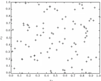
As a rst trial, four hundred training data were sampled randomly from the input domain of 0 x1; x2 1 (see Figure 3) and the corresponding true
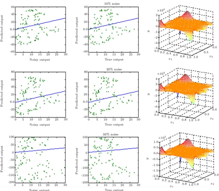
underlying responses were computed using Equation 8. The normalization of input space does not create any limitation for practical applications, but extremely enhances the selection of isotropic spreads. The true underlying responses were then contaminated with 10, 20 and 50 percent noise levels and the corresponding noisy outputs are shown in Figure 4. The blue line indicates that y = x.
Figure 4. Training data with dierent noise levels.
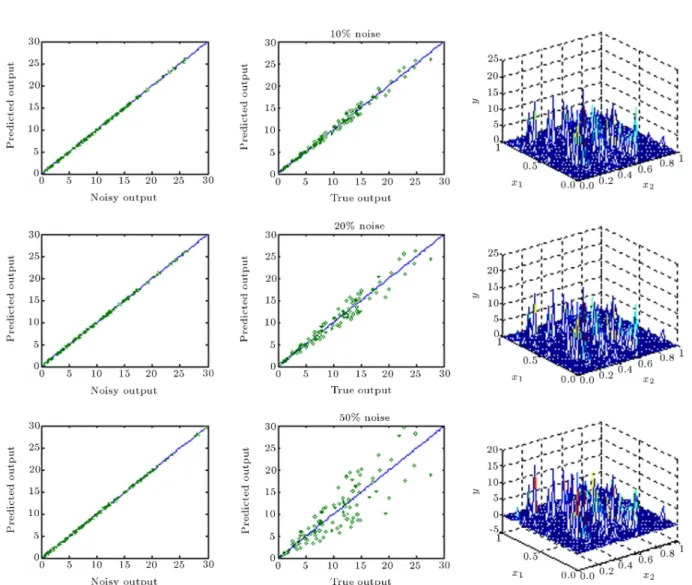
Figure 5a. Generalization performance of regularization network for various noise levels in the absence of regularization ( = 0:01).
The above noisy data sets were used for training three separate regularization networks with dierent isotropic spreads, each with 100 Gaussian basis func-tions centered at the training data points. Figures 5a to 5c show the 3D generalization performance of these networks on a 5050 uniform grid for the isotropic
spreads of = 0:01; 0:1 and 0:5 and noise levels of 10%, 20% and 50%, in the absence of regularization ( = 0). All 2D diagrams correspond to recall performances of regularization networks for the training data set. As before, the blue line indicates that y = x.
net-Figure 5b. Generalization performance of regularization network for various noise levels in the absence of regularization ( = 0:1).
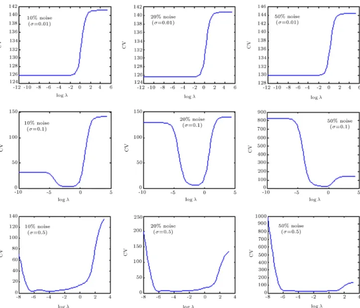
works with extremely small spreads ( = 0:01) will t the noise in the absence of regularization. Such networks exactly reproduce the noisy data but per-form inadequately between the training data points. The reason for this is that the Green matrix of the regularization network tends to an N N identity matrix for very small spreads. Such matrices are very well behaved and invertible. Since both the Green matrix and its inverse are identical, the network exactly recovers the training data points. On the other hand, the Gaussian basis functions are exceedingly narrow and, as can be seen, the network cannot produce a sucient response between the training data points. Increasing the value of the isotropic spread to 0.1 in the absence of regularization, although tting the noise, leads to a smoother hyper-surface with large oscillations (see the magnitude of Y on the 3D plots of
Figure 5b). Figure 5c shows that a similar situation can happen for the case of = 0:5. The reason for these large oscillations is the ill-conditioning of the Green matrix. This phenomenon occurs because of the exces-sive overlap between adjacent centers at relatively large spreads. Inversion of such a nearly singular matrix can lead to extremely oscillatory synaptic weights and produces a fairly smooth but unreliable surface with tremendously large responses.
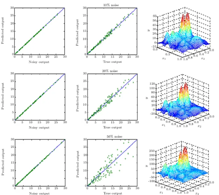
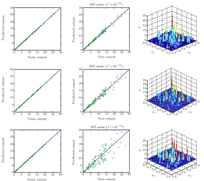
Employing the regularization technique can alle-viate the ill-conditioning problem of the Green matrix, due to the overlap of large spreads, but will not cure the inadequacy of the model (network) for very small spreads. This issue is clearly demonstrated by using the same data set for training the previous networks with an optimum level of regularization (). The
Figure 5c. Generalization performance of regularization network for various noise levels in the absence of regularization ( = 0:5).
the generalization performances of these networks on a 50 50 uniform grid for = 0:01; 0:1 and 0.5. The Leave-One-Out (LOO) Cross Validation (CV) criterion was used to compute the optimum level of regularization. As mentioned earlier, the 2D plots show the recall performances of the regularization networks.
The above gure clearly shows that the inade-quacy of the model (due to small isotropic spreads) cannot be alleviated by the optimum level of regular-ization. As shown in Figure 7, the Cross Validation (CV) criterion does not possess any minima for various noise levels with = 0:01. On the other hand, when the isotropic spread is large enough to provide an appropriate model for the data set, the Green matrix may become ill-conditioned and the CV criterion shows a clear minimum. The optimum level of regularization
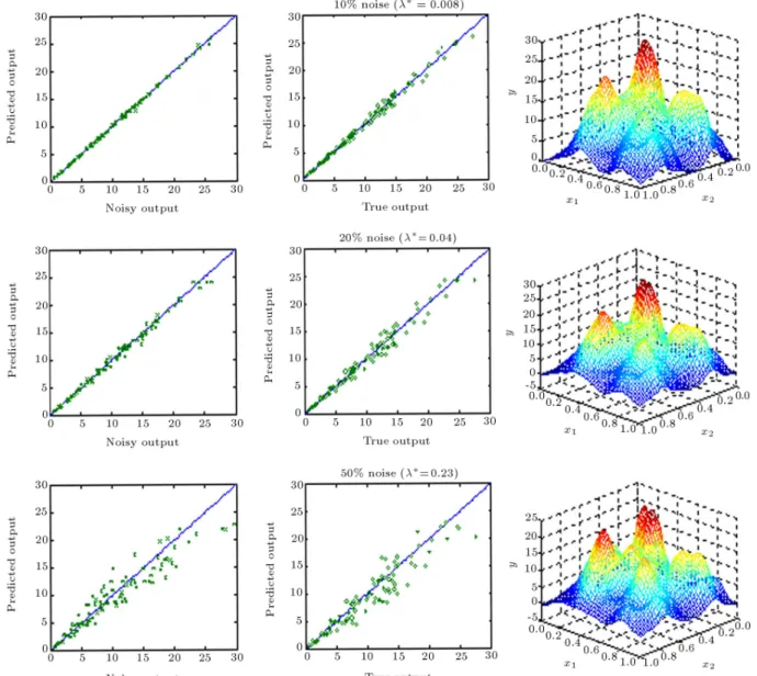
eliminates the ill-conditioning problem and leads to a reasonable generalization performance, as shown in Figures 6b and 6c.
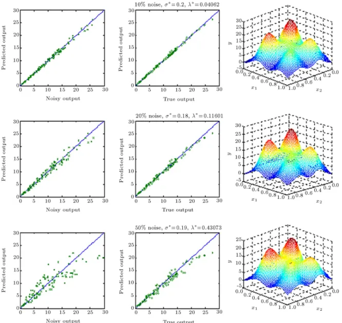
It is interesting to note that a regularization network with a proper choice of spread and an optimum level of regularization can lter out the noise (instead of following it) and capture the true response from the highly noisy data sets (see 2D plots of Figure 6c for 50% noise). It is also clearly visible that, with a reasonable value of isotropic spread, the regularization network is able to reconstruct the general features of the true underlying surface hidden in a set of noisy data. It should also be noted that the predicted surface is still oscillatory and cannot provide the exact true responses. Therefore, a mechanism should be devised to nd the optimal value of isotropic spread () for a given data
Figure 6a. Generalization performance of regularization network for various noise levels at the optimum level of regularization ( = 0:01).
Closer examination of Figures 6a to 6c reveals that the optimum level of regularization, (), is
strongly correlated with the value of the isotropic spread. A plot of versus for various noise levels
on Figure 8 shows a clear maximum; the corresponding value of the isotropic spread can be regarded as the optimum value of spread () for the regularization
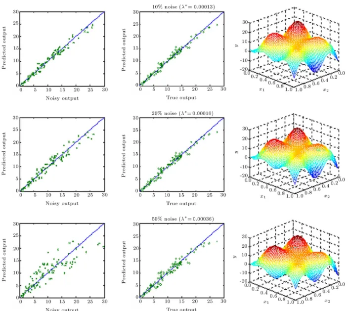
network under consideration. On the other hand, the cross validation criterion decreases monotonically and does not provide any maximum or minimum, as shown in Figure 8. Evidently, such criterion cannot be used to select the optimum value for the isotropic spread. Figure 9 illustrates the generalization per-formance of the regularization networks at optimum values of isotropic spread and the corresponding op-timum level of regularization for various noise lev-els.
As can be seen in Figure 8, the optimum value of the spread is independent of noise level, but further investigation shows that it is strongly dependent on the number of training data points.
It is also interesting to note that the trained network with an optimal isotropic spread at an opti-mum level of regularization does not follow the noise, but tries to capture the true underlying trend hidden in the remarkably noisy training sets (see Figure 9). The above discussion proves that regularization is essential to prevent spurious oscillation caused by over-tting of the noisy data. More signicantly, using an appropriate value of and an optimal level of regularization determined by the CV criterion recovers the true underlying surface remarkably well from the above set of limited and noisy data.
Figure 6b. Generalization performance of regularization network for various noise levels at the optimum level of regularization ( = 0:1).
two local maxima for relatively low noise levels. Fig-ure 10 shows the generalization performance of the regularization networks with isotropic spreads of 0.03 (corresponding to rst local maxima) for 10 and 20 percent noise levels. Evidently, the rst maxima cannot de-correlate the isotropic spread and level of regularization.
We close this discussion of regularization networks by giving a justication for the existence of a threshold value for the isotropic spread, , based on an approx-imate measure of the degrees of freedom that can be sustained by the data. For a model with M parameters representing given N observations, the eective degrees of freedom are equal to N M. Using the denition of the smoother matrix as [17]:
H() = G(G + I) 1: (14)
For model comparisons, the approximate degrees of freedom, which give an indication of the amount of tting that H does, are dened as the tr(H) (sum of the eigenvalues of matrix H). Figure 11 illustrates the variations of the optimal levels of regularization, , and the corresponding approximate degrees of
freedom df()= tr (H()), with the isotropic spread
of the Gaussian basis functions used in a regularization network.
It is clear that threshold occurs near the point where the approximate degrees of freedom have a minimum. Using threshold , therefore, enables us to select the approximate degrees of freedom required to t the underlying surface. Smaller introduces larger degrees of freedom leading to spurious oscillations, while larger limits the degrees of freedom and leads to over-smoothing.
Figure 6c. Generalization performance of regularization network for various noise levels at the optimum level of regularization ( = 0:5).
CONCLUSION
Chemical engineering data are expensive to collect and are always contaminated with some level of noise. E-cient algorithms are required to lter out the noise and capture the true underlying trend from the noisy data sets. Regularization networks are inherently equipped with proper means to perform such a demanding task. This paper was aimed exclusively at an important class of feed-forward neural networks with a single hidden layer (Regularization Networks), which have a solid mathematical foundation. In the majority of reported applications, the regularization network has been employed with Gaussian radial basis functions with a constant isotropic spread.
It is shown that the optimal value of regular-ization parameter, , is highly correlated with the
isotropic spread, , an obvious point that has received surprisingly little attention to date. An illustrative example was used to clearly demonstrate the strong correlation between and . A signicant
contribu-tion of the present article is the development of a con-venient procedure for de-correlating these parameters and selecting the optimal values of and .
It is also clearly demonstrated that the eective degrees of freedom, df(; ), of a regularization net-work is a function of both the regularization level, , and the isotropic spread, . A readily calculable measure of the approximate degrees of freedom of a regularization network was introduced, which may be used to de-couple and . The plot of df(; )
against provides a curve which exhibits a minimum. This minimum is an approximate measure of the degrees of freedom which can be reasonably sustained
Figure 7. CV criterion vs. level of regularization for various noise levels and spreads.
Figure 8. Optimum level of regularization and the corresponding cross validation criterion vs. isotropic spreads for various noise levels.
by the noisy data set and which can be used to provide the best value for the isotropic spread, . The use
of the eective degrees of freedom for this purpose leads to a signicant improvement in the performance of the regularization network and, to our knowledge,
has not been previously reported. Applications of the above algorithm on several case studies in the elds of characterization and optimization of porous materials and in the modeling of membrane processes are presented elsewhere [19,20].
Figure 9. Generalization performance of regularization network at optimum value of isotropic spread and optimal regularization level.
Figure 10. Generalization performance of regularization network with spreads corresponding to the rst local maxima at for relatively low noise levels.
Figure 11. Variations of the degrees of freedom and optimum regularization level with optimum isotropic spread of the Gaussian basis functions regularization network.
REFERENCES
1. Himmelblau, D.M. and Hoskins, J.C. \Articial neural network models of knowledge representation in chem-ical engineering", Computers and Chemchem-ical Engineer-ing, 12, pp. 881-890 (1988).
2. Venkatasubramanian, V. and Chan, K. \A neural net-work methodology for process fault diagnosis", AIChE Journal, 35, pp. 1993-2002 (1989).
3. Watanabe, K., Matsuura, I., Abe, M., Kubota, M. and Himmelblau, D.M. \Incipient fault diagnosis of chemical engineering processes via articial neural networks", AIChE Journal, 35(11), pp. 1803-1812 (1989).
4. Shahsavand, A. \Optimal and adaptive radial basis function neural networks", PhD. Thesis, University of Surrey, UK (2000).
5. Carr, J.C., Beatson, R.K., McCallum, B.C., Fright, W.R., McLennan, T.J. and Mitchell, T.J. \Smooth surface reconstruction from noisy range data", ACM GRAPHITE 2003 Proceeding, Melbourne, Australia, pp. 119-126 (2003).
6. Haykin, S., Neural networks: A Comprehensive Foun-dation, Second Ed., New Jersey, Prentice Hall (1999). 7. Poggio, T. and Girosi, F. \Regularization algorithms for learning that are equivalent to multilayer net-works", Science, 247, pp. 978-982 (1990).
8. Poggio, T. and Girosi, F. \Networks for approximation and learning", Proceedings of the IEEE, 78, pp. 1481-1497 (1990).
9. Hunt, K.J., Sbarbaro, D., Zbikowski, R. and Gawthrop, P.J. \Neural networks for control systems -a survey", Autom-atic-a, 28(6), pp. 1083-1112 (1992). 10. De Nicolao, G. and Ferrari-Trecate, G.
\Regulariza-tion networks: Fast weight calcula\Regulariza-tion via kalman ltering", IEEE Trans. Neural Networks, 12(2), pp. 228-235 (2001).
11. Carr, J.C., Beatson, R.K., Cherrie, J.B., Mitchell, T.J., Fright, W.R., McCallum B.C. and Evans, T.R. \Reconstruction and representation of 3D objects with radial basis functions", ACM SIGGRAPH 2001 Pro-ceeding, CA, USA, pp. 67-76 (2001).
12. Micchelli, C.A. \Interpolation of scattered data: Dis-tance matrices and conditionally positive denite functions", Constructive Approximation, 2, pp. 11-12 (1986.)
13. Powell, M.J.D., Radial Basis Function for Multivari-ate Interpolation, a Review, Clarendon Press, Oxford (1987).
14. Powell, M.J.D. \Radial basis function approximation to polynomials", Proceedings of 1987 Dundee biennial Numerical Analysis Conference, pp. 223-241 (1987). 15. Sugiyama, M. and Ogawa, H. \Optimal design of
reg-ularization term and regreg-ularization parameter by sub-space information criterion", Neural Networks, 15(3), pp. 349-361 (2002).
16. Golub, G.H. and Van Loan, C.G., Matrix Computa-tions, Johns Hopkins University Press, Baltimore, 3rd Ed. (1996).
17. Hastie, T.J. and Tibshirani, R.J., Generalized Additive Models, Chapman and Hall, London, First Ed. (1990). 18. Golub, G.H., Heath, M. and Wahba, G. \Generalized cross validation as a method for choosing a good ridge parameter", Technometrics, 21(2), pp. 215-223 (1979). 19. Shahsavand, A. and Ahmadpour, A. \Application of optimal RBF neural networks for optimization and characterization of porous materials", Computers and Chemical Engineering, 29, pp. 2134-2143 (2005). 20. Shahsavand, A. and Pourafshari, M. \Neural network
modeling of hollow ber membrane process", Journal of Membrane Science, 297, pp. 59-73 (2007).