61
Functional Duration Models for Highway Construction Projects in
Nigeria
B. S. Waziri, B. Kadai and A.T. Jibrin
Department of Civil and Water Resource Engineering, University of Maiduguri, Nigeria * Corresponding Author: E-mail:
Abstract
Construction duration significantly influences funding, financing and resources allocation decisions that take place early in project design development. This study attempts to develop through regression analysis highway construction duration models by incorporating relevant predictor variables having statistically significant relationship with highway completion time. Historical data of highway projects initiated and completed between 2007 and 2012 were considered to enable the collection of homogenous data in terms of time, cost and other economic variables. Three multiple regression models were developed in the form of linear, semi-log and log-log transformations. The results of the analysis showed that all the three models are statistically significant and have good fit to the data with R2 values of 0.546, 0.631 and 0.940 respectively. The performances of the models were established by measuring their prediction accuracy and goodness of fit over a test sample of 15 successful projects. The result revealed that the log-log model outperformed the other models with an average % Error of -3.64%, Maximum error of 16.2% and Mean Absolute Percent Error (MAPE) of 6.87%. These results compare favourably with past studies which have shown that traditional methods of duration estimation at early project stages have values of MAPE typically in the order 10-20%.
Key Words:
Highway projects, Duration Models, Regression Analysis, Nigeria1. Introduction
Time and cost are extremely important parameters of construction projects essential for planning, feasibility analysis, budget allocation decisions, project monitoring and litigation which often becomes the basis for ascertaining other estimates [1, 2, 3 and 4]). Shr and Chen [5] considered time and cost as critical benchmark for evaluating the performance of construction projects which enables effective budgeting and adequate financing. They are also used as an indicator of contractors efficiency, professionalism and competence which reflects the ability of the contractor to organize and control site operation, to appropriately allocate resources and to manage the flow of information to and from the design team and among all other project parties [6 and 7]. Determining optimum durations for projects at the early phase is a veritable exercise for incorporating realistic schedule in the bid package as the indirect cost associated with capital projects is highly dependable on the duration of the project. The prediction of construction duration represents a
problem of continual concern to both state highways and contractors because highway construction duration is not always a simple problem, because of myriad of factors influencing its accuracy such as project size, type, location, year, types of materials used and method of construction adopted [8]. However, [9, 10 & 11] have shown that construction delay is a major factor bedevilling the Nigerian construction industry because almost all projects are completed at durations much longer than their initially planned duration. Odusami and Olusanya [12] reported that construction projects in Lagos experience about 51% delay which could be attributed to the numerous complex factors influencing the construction process. Therefore, it is imperative to develop at the early phase the probable completion duration of highway projects to enable practical estimation and feasibility study.
2. Statement of Research Problem
Despite the importance of accurately and reliably predicting construction duration, early in the project development lifecycle, few tools, practicesand procedures are presently available for application [13]. The building construction industry has explored this area and found results in statistical regression analysis and artificial intelligence. Such analysis has led to the understanding of the components that influence construction durations and their relationships [14, 15, 16, 17 and 18]. The highway construction industry has not demonstrated such results and both clients and contractors in the industry recognized the need for improved conceptual design level estimating practices. Highway construction duration estimates are prepared very early in project design and based on individual experience on similar projects [13], which are more often than not unrealistic and inaccurate. The alternative methods adopted by most contractors usually require more detailed scheduling tool and assumptions pertaining to project information such as material quantities and activities involved. Such approaches are time consuming and characterised by lack of information at the early phase.
However, the highway construction industry calls for a pragmatic models and robust methods for fast and efficient prediction of construction duration at the planning phase. This study therefore attempts to develop a functional model based on historical data for the prediction of highway project duration by incorporating relevant predictor variables.
3. Highway Duration Models
Duration models are generally developed for reliable prediction of construction durations based on available information at a particular phase of project. Construction duration are estimated either based on clients time constraints or through a detailed analysis of work to be done and resources available using estimates of time requirement for each specific activity. Most predictive models are based on historical project data of successful projects prepared by construction professionals for determining project duration which has been a subject of many studies [5, 10, 19, 20 and 21].
The first empirical modelling of construction time performance (CTP) was carried out by [19] in Australia. The resulting model is referred to as the Bromilow’s Time-Cost Model (BTC) which enables construction duration to be determined based on
estimated final cost. Shr and Chen [5] developed a model to illustrate cost-time relationship of highway projects using data obtained from the Florida Department of Transportation. The model provides state highway agencies and contractors with increased control and understanding regarding the time value of highway construction projects. However the model was not suitable for projects with great degree of change order. Martin [22] established a forecasting model using regression analysis based on actual time of building construction in the United Kingdom. The result presents a tool to aid clients and contractors in estimating or benchmarking the construction duration at the earliest stage of future projects. Hoffman et al. [23] developed multiple regression model to predict highway construction duration by improving the parameters that impact construction duration. The data for the study were examined using BTC Model and regression analysis. The regression model compared favourably with the BTC Model with minimum error. Assadulla [24] also attempted to develop highway duration model using stepwise regression and Artificial Neural Network. The outcome of the study revealed that the ANN represented higher accuracy and reliability. Petruseva [25] conducted a research and developed a forecasting model for construction time using support vector machine. The analysis involved 75 objects structured in the period 1999-2011 in the Federation of Bosnia and Herzegovina. The results showed an accurate presentation for building work and suggested it to be useful for planning in the construction industry. Waziri and Yusuf [26] made an attempt to validate the BTC model using highway construction data in Nigeria. The model indicated a K value (which demonstrates a general level of time performance) of 2.8 which is considered very low compared to values obtained by previous studies for other categories of construction. The model also showed a weak prediction efficacy with MAPE of 19% over a test sample. This may be attributed to the non inclusion of other duration influencing factors apart from cost in the model. Therefore it is necessary to consider other relevant variables in order to accurately and reliably estimate the probable completion time of highway project for the purpose of feasibility studies, planning, budgeting and adequate financing.
63
4. Methodology
Data for analysis and modelling were obtained from the records of completed highway projects from clients and contractors in Gombe and Bauchi states in North Eastern Nigeria. Dataset of 57 successful highway projects initiated and completed between 2007 and 2014 were considered to enable the collection of homogenous data in terms of time and cost. Projects that made up the survey population were restricted to those with contract value of more than ₦100,000,000 which are considered to demonstrate reasonable scope and complexity [26]. 75% of the projects (42) were used for developing the models while the remaining 25% (15) were used for evaluation and validation of the models. Three regression analyses viz; linear, semi-log, and log-log were established incorporating four (4) significant variables affecting highway construction duration (measured in calendar days) with the view to improving the BTC model which considers only the cost of construction. The variables considered and included in the models as input variables based on selection by [27] are:
i. Estimated project cost per unit length (₦) ii. Number of culverts along the highway
stretch
iii. Thickness of pavement materials (m) iv. Road length (m)
Linear regression analysis was employed to describe the value of dependent variable on the basis of the independent variables. The linear regression equation is as presented in equation (1)
4 4 3 3 2 2 1 1 0
1 x x x x
y
(1)Semi-log regression analysis was also employed for developing a transformed regression model. It is identified to produce best statistical results in terms of parameter significance [28]. Semi-Log regression is of the form presented in equation (2)
4 4 3 3 2 2 1 1 0
lny
x
x
x
x (2) Log-log model having all the variables transformed to the logarithmic form was also developed; it is of the form presented in equation (3)4 4 3 3 2 2 1 1 0 ln ln ln ln ln x x x x y
(3)The models were then evaluated for goodness of fit and prediction performance by comparing the prediction results over a test sample using Mean Absolute Percent Error (MAPE) and Mean Square Error (MSE).
5. Results and Discussions
5.1 Relationship of input variables
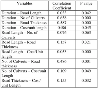
The relationships of the input variables were examined to determine the existence of autocorrelation between them. The product moment correlation which illustrates the relationship between them was computed and presented in Table 1.
Table 1 Pearson product moment correlations between each pair of input variables Variables Correlation
Coefficient
P value Duration – Road Length 0.033 0.042 Duration – No of Culverts 0.658 0.000 Duration – Road Thickness 0.587 0.000 Duration – Cost/unit length 0486 0.045 Road Length – No. of
Culverts
0.076 0.063 Road Length – Road
Thickness
0.157 0.321 Road Length – Cost/Unit
length
0.053 0.000 No. of Culverts – Road
thickness
0.486 0.001 No. of Culverts – Cost/unit
Length
0.109 0.049 Road Thickness – Cost/
unit Length
0.155 0.032
The product moment correlation between each pair of the variables measures the relationship between the variables. These coefficients range between -1 and +1. P-values below 0.05 indicate statistically significant non-zero correlations at the 95% confidence level. From the result, the pair of variables having P-value greater than 0.05 is road length and road thickness with a value of 0.321 indicating zero correlation at the 95% confidence level.
64
Three different regression models namely linear, semi-log and log-log were developed. The semi-log has the dependent variables transformed to the logarithmic form while in the log-log model all the variables were transformed into their respective logarithmic form.5.2.1 Linear Regression Model (M1)
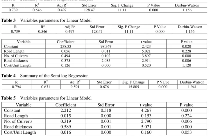
The summary of the multiple regression model in which all the variables were considered without transformation is presented in Table 2 while the equation of the fitted model is presented in equation (4).
From the results, the R2 value of 0.546 indicates that 54.6% of the variability in construction duration is explained by the model indicating significant relationship between the dependent and the independent variables. Since the p value is also less than 0.005 it indicates that there is a statistically significant relationship between the variables at the 95% confidence level. The parameter estimate of the independent variables is presented in Table 3.
The results of the coefficients revealed that the p value of the variables road length and cost per unit length are greater than 0.05 indicating weak association between the independent variables and
construction duration as presented by the model. The equation of the fitted model is presented in eqn. 4.
5.2.2 Semi-Log Regression
In the semi-log regression analysis, the dependent variable of the regression analysis was transformed to its logarithmic form in order to improve the performance of the model. The data for the duration is transformed while the data of the independent variables were entered raw. The summary of the regression is presented in Table 4.
From the result of the analysis, the R2 value of 0.631 indicates that 63% of the variability in the data is accounted for by the model. The R value of 0.794 shows significant association between the dependent variable and the independent variables. The p value of <0.001 suggests significant relationship between the variables at the 95% confidence level. The parameter of the variables of the semi-log regression model is presented in Table 5.
RoadLength
Duration 283.33 0.056
0.494No.ofCulverts0.375Road
RoadThickness0.126Costperunitlength (4) Table 2 Summary of Linear Regression analysis
R R2 Adj R2 Std Error Sig. F Change P Value Durbin-Watson
0.739 0.546 0.497 128.47 11.11 0.000 1.156
Table 3 Variables parameters for Linear Model
R R2 Adj R2 Std Error Sig. F Change P Value Durbin-Watson
0.739 0.546 0.497 128.47 11.11 0.000 1.156
Variable Coefficient Std Error t value P value
Constant 238.33 98.367 2.423 0.020
Road Length 0.056 0.011 5.021 0.228
No. of Culverts 0.494 0.102 3.897 0.000
Road thickness 0.375 2.035 2.914 0.006
Cost/Unit Length 0.126 0.000 0.520 1.120
Table 4 Summary of the Semi log Regression
R R2 Adj R2 Std Error Sig. F Change P Value Durbin-Watson
0.794 0.631 9.591 0.676 15.805 0.000 1.941
Table 5 Variables parameters for Linear Model
Variable Coefficient Std Error t value P value
Constant 2.212 0.518 4.267 0.000
Road Length 0.015 0.000 0.153 0.224
No. of Culverts 0.319 0.001 2.790 0.006
Road thickness 0.589 0.001 5.071 0.000
65
The results of the coefficients of the variables indicate that the p value corresponding to the variables road length and road thickness are greater than 0.005 suggesting the weak contribution of the variables to the model. This may be attributed to the fact that some of the properties contained in those variables may be contained in some of the variables showing strong association. The semi-log model is presented is represented by equation 5.
RoadLength
Duration
Ln 2.212 0.0015
0.312No.of Culverts0.589RoadThickness
0.016Costperunitlength (5)
5.2.3 Log-Log Regression
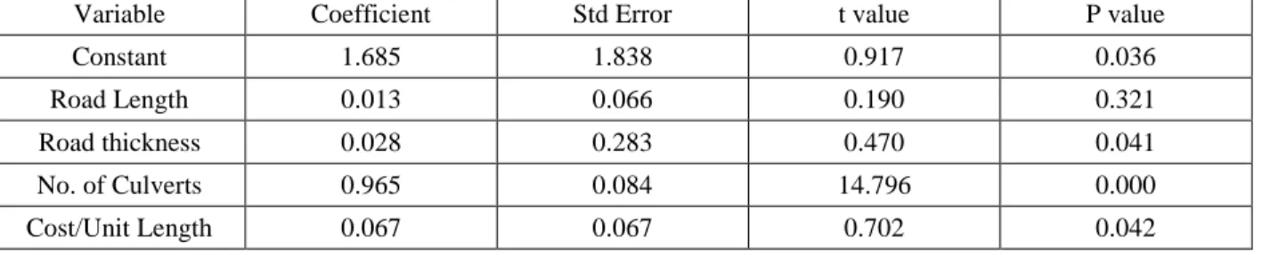
In order to further test for the possible improvement of the earlier models, both dependent and the independent variables were transformed to the logarithmic form to have the log-log regression model. The summary of the analysis is presented in Table 6.
From the analysis, 94% of the variability in duration is explained by the model as indicated by the R2 value of 0.941. The adjusted R-squared statistics which is more suitable for comparing models with different numbers of independent variables is 93.4%. The standard error of the estimate shows the standard deviation of the residuals to be 0.272. This value can be used to construct prediction limits for new observations. The p value of <0.001 indicates that the relationship is significant at 99% confidence level. Durbin-Watson statistics of 1.163 is use to test the residuals to determine if there is any significant correlation in which the data occur. Since the p value is less than 0.005, there is indication of serial autocorrelation in the residuals. The result of the parameters for the variable in the log-log model is presented in Table 7.
From the results of the parameters of the independent variables, the highest p value on the independent variables is 0.321 belonging to road length indicating that the variable is not significant at the 95% confidence level. This is followed by 0.042
belonging to cost/unit length and 0.041 belonging to road thickness both values less than 0.05, indicating significance at the 95% confidence level. The equation of the model is presented in equation 6.
RoadLength
Duration
Ln 1.685 0.013*ln
0.028*lnNo.ofCulverts0.965*lnRoad
Thickness0.067lnCost perunitlength (6) The summary of the three models are presented in Table 8 showing regression results of individual analysis and errors between predicted and observed values.
5.3 Evaluation of Models
5.3.1 Prediction Performance
The prediction performance of the models was established by comparing their predictions over a test sample. The sample consists of dataset of 15 successfully completed highway projects. The model equations were constructed using Microsoft excel spreadsheet and were used to predict the construction durations of the test sample. Mean absolute percent errors (MAPE), minimum, maximum and average errors were calculated based on the models’ predictions of the actual durations. The result is presented in Table 9.
The results of the evaluation revealed that the linear, semi-log and log-log models have average prediction errors of -7.38, -63.24 and -3.64 % respectively which suggests that the log-log model has the smallest average error over the test sample. The result also revealed that the log-log model has the smallest value of MAPE of 6.87% demonstrating a good performance. The logarithmic model therefore outperformed the linear and the semi-log models in all the error terms.
5.3.2 Prediction Accuracy of Log-Log Model
The calculated output of the test samples by the log-log model revealed that 73.33% of the test samples were underestimated while 26.67% were overestimated. The range of underestimating varies from 10.29% to 1.03% with an average value of -7.23%. The range of overestimating varies from 0.10% to 16.20% with an average value of 7.51%. These ranges show that the model is skewed to underestimating the test samples. On the overall, the log-log model has an average % error of -3.64%, a
maximum % error of 16.21% and a MAPE of 6.87%. The value of MAPE of 6.87% is a very good performance; it is within the acceptable range of
10 % by [3],
25% for early estimates by [29].6. Conclusions
Reliable and accurate estimates of highway project durations are desired by state highway agencies and contractors for inclusion in the bid package. In the study, four relevant predictor variables namely road length, road thickness, number of culverts and cost per unit length were included in the model in order to improve the performance of the models. This is because earlier attempts to modelled using only cost of construction as the independent variable in line with BTC model was found to be unsatisfactory. The results of the study revealed that the prediction performance of the log-log model in
terms of goodness of fit and prediction accuracy was better than that of the other models. This may be attributed to the transformation of the variables to the logarithmic form. The model is useful to both clients
and contractors because of its ability o predict construction duration at the early project stage, since the information necessary as input variables can be extracted from scope designs and early estimates. Due to its simplicity, it can be handled using Microsoft excel or a simple computer programme. The main limitation of regression models is that the collinearity of the predictor variables may affect the prediction performance of the regression model.
7. References
[1] Bowen, P.A., Hall, K.A. Edwards, P.J., Pearl, R.G. and Cattell, 2000. Perceptions of Time, Cost and Quality Management of Building Table 6: Summary of Log-Log Regression
R R2 Adj R2 Std Error R Square
Change
Sig. F Change
P Value Durbin-Watson
0.970 0.940 0.934 0.272 0.940 145.03 0.000 1.163
Table 7: Parameters estimates of Variables for Log-Log Model
Variable Coefficient Std Error t value P value
Constant 1.685 1.838 0.917 0.036
Road Length 0.013 0.066 0.190 0.321
Road thickness 0.028 0.283 0.470 0.041
No. of Culverts 0.965 0.084 14.796 0.000
Cost/Unit Length 0.067 0.067 0.702 0.042
Table 8: Summary of the models
Model R R2 Adj R2 Std Error Sig. F Change P Value
Linear 0.739 0.546 0.497 128.47 11.11 <0.000
Semi-log 0.794 0.631 0.591 0.676 15.805 <0.0001
Logarithmic 0.970 0.940 0.934 0.272 145.03 <0.0001
Table 9: Prediction Performance of Models
Model Average Error (%) Min Error (%) Max Error (%) MAPE (%)
Linear – 7.38 –96.95 146.19 43.36
Semi-log –63.24 –83.34 –74.40 57.23
67
Projects. The Australian Journal of Construction Economics and Building. Vol. 2(2). pp 48-56[2] Chan, A.P.C and Chan, D.W.M. 2002. Benchmarking project construction time performance: the case of Hong Kong, Project management-impresario of the construction industry held 22nd-23rd March 2002, Hong Kong.
[3] Ogunsemi, D.R and Jagboro, G.O. 2006. Time-Cost model for building projects in Nigeria. Construction management and economics. Vol. 24(1). pp 253-258.
[4] Skitmore, R.M. and Ng, S.T. 2003. Forecast Models for Actual Construction Time and Cost, Building and Environment. Vol. 8(8). pp 1075-1083.
[5] Shr, F. and Chen W.T 2006. Functional Model of Cost and Time For Highway Construction Projects. Journal of Marine Science and Technology, 14 Vol. (3). pp 127-138.
[6] Ireland, V. 1986. “A comparison of Australia and US building performance for high-rise buildings”. University of Technology, Sydney, Australia: School of Building Studies.
[7] CIDA 1993. Project Performance update – A Report on the Cost and Time Performance of Australian Building Projects Completed 1988-1993, Construction Industry Development Agency, Australia.
[8] Hegazy, T. and Ayed, A. 1998. Neural network model for parametric cost Estimation of highway projects Journal of Construction Engineering and Management, ASCE Vol. 124(3). pp 210-218.
[9] Mbachu, J.I.C. and Olaoye, G.S. 1999. Analysis of Major Delay Factors in Building Projects Execution. Nigerian Journal of Construction Technology and Management. Vol. 2(1). pp 81-86.
[10] Izam, Y.D. and Bustani, S.A. 1999. Predictive Duration Models for Building Construction in Nigeria. Journal of Environmental Sciences. Vol.3(2). pp 125-131.
[11] Olupopola, F.O., Emanuel, O.O., Adeniyi, M.F. and Kamaldeen, A.A. 2010. “Factors Affecting Time Performance of Buildings”. Proceedings of the Construction, Building and Real Estate Research Conference of the Royal Institution of Chartered Surveyors, Dauphine, Paris.
[12] Odusami, K.T. and Olusanya, O.O. 2000. Client’s Contribution to delays on Building completion, The Quantity Surveyor, Vol. 30(1). pp 30-33.
[13] Williams, R. 2008. Development of Mathematical Model for Preliminary Predictions of Highway Construction Duration. PhD Thesis submitted to the Faculty of Virginia Polytechnic Institute and State University, Blacksburg, VA. [14] Bromilow, F.J., Hinds, M.F., and Moody, N.F.
1980. AIQS Survey of Building Contact Time Performance. Building Economist. Vol. 19(2), 79-82.
[15] Nkado, R.N. 1992. Construction Time Information System for the Building Industry. Construction Management and Economics. Vol. 10. pp 489-509.
[16] Chan, D.W.M. and Kumaraswamy, M.M. 1995. A Study of Factors Affecting Construction Durations in Honk Kong. Construction Management and Economics. Vol. 13. pp 319-333.
[17] Chan, A.P.C. 1999. Modelling Building Durations in Hong Kong. Construction Management and Economics. Vol. 17. pp 189-196
[18] Skitmore, R.M. and Ng, S.T. 2001. Australian Project Time-Cost Analysis: Statistical Analysis of Inter-temporal trends. Construction Management and Economics. Vol.19. pp 455-458.
[19] Maghrebi, M., Afshar, A. and Maghrebi, M.J. 2013. A Novel Mathematical Model for
determining Time-Cost trade-off Based on Path Constraints. International Journal of Construction Engineering and Management. Vol. 2(5). pp 137-142.
[20] Levinson, D. and Karamalaputi, K 2003. Predicting the Construction of New Highway Links. Journal of Transportation and Statistics. Vol. 6(2). pp 2-9.
[21] Bromilow, F.J. 1969. Contract Time Performance Expectations and the Reality. Building Forum. Vol.1(3). pp 70-80.
[22] Martins, J., Burrows, J.K. and Pegg, I 2006. “Predicting construction durations of buildings Projects”. XXIII FIG congress, Munich, Germany.
[23] Hoffman, G.J., Thai, A.E., Web, T.S. and Weir, J.D. 2007. Estimating Performance Time for Construction of Projects. Journal of Management in Engineering. Vol. 23(4). pp 193-199.
[24] Aasadullah, A. 2010. Development of Neural Network Models for Prediction of Highway Construction Cost and Project Duration. M.Sc. Thesis Submitted to the Faculty of The Russ College of Engineering and Technology of Ohio University.
[25] Petruseva, S., Zicska-panakovska, V and Zudo, V. (2013). Predicting ConstructionDuration with Support Vector Machine. International Journal of Research in Engineering and Technology. Vol. 2(11). Pp 12-24.
[26] Waziri, B.S. and Yusuf, N. 2015. Application of Bromilow’s Time-Cost Model for Highway Projects in Nigeria. Arid Zone Journal of Engineering Technology and Environment. Vol. 9(1) In press.
[27] Jibrin, A.T. 2014. Development of Pragmatic Time-Cost Model for Highway projects in Nigeria: A Case study of Bauchi Township Roads. Unpublished B.Eng. Thesis Submited to the Department of Civil and Water Resources Engineering, University of Maiduguri.
[28] Stoy, C. and Schalcher, H. R. 2007. Residential Building Cost Drivers and indicators. Journal of Construction Engineering and Management,. Vol. 133(2). pp 139-145.
[29] Schexnayder, C. J. and Mayo, Richard E., 2003.Construction Management Fundamentals, McGraw-Hill Higher Education, Boston, MA.