DRAFT
D. Vermeir
Dept. of Computer Science
Vrij Universiteit Brussel, VUB
[email protected]
S R
E
V
I N U
ITEIT E
J
I R V
BR
US
SE
L
E C N
I
V
RETEN EBR
AS
A I T N E
I
C
S
1 Introduction 6
1.1 Compilers and languages . . . 6
1.2 Applications of compilers . . . 7
1.3 Overview of the compilation process . . . 9
1.3.1 Micro . . . 9
1.3.2 x86 code . . . 10
1.3.3 Lexical analysis . . . 12
1.3.4 Syntax analysis . . . 13
1.3.5 Semantic analysis . . . 14
1.3.6 Intermediate code generation . . . 15
1.3.7 Optimization . . . 16
1.3.8 Code generation . . . 17
2 Lexical analysis 18 2.1 Introduction . . . 18
2.2 Regular expressions . . . 24
2.3 Finite state automata . . . 26
2.3.1 Deterministic finite automata . . . 26
2.3.2 Nondeterministic finite automata . . . 28
2.4 Regular expressions vs finite state automata . . . 31
2.5 A scanner generator . . . 32
3 Parsing 35
3.1 Context-free grammars . . . 35
3.2 Top-down parsing . . . 38
3.2.1 Introduction . . . 38
3.2.2 Eliminating left recursion in a grammar . . . 41
3.2.3 Avoiding backtracking: LL(1) grammars . . . 43
3.2.4 Predictive parsers . . . 44
3.2.5 Construction of first and follow . . . 48
3.3 Bottom-up parsing . . . 50
3.3.1 Shift-reduce parsers . . . 50
3.3.2 LR(1) parsing . . . 54
3.3.3 LALR parsers and yacc/bison . . . 62
4 Checking static semantics 65 4.1 Attribute grammars and syntax-directed translation . . . 65
4.2 Symbol tables . . . 68
4.2.1 String pool . . . 69
4.2.2 Symbol tables and scope rules . . . 69
4.3 Type checking . . . 71
5 Intermediate code generation 74 5.1 Postfix notation . . . 75
5.2 Abstract syntax trees . . . 76
5.3 Three-address code . . . 78
5.4 Translating assignment statements . . . 79
5.5 Translating boolean expressions . . . 81
5.6 Translating control flow statements . . . 85
5.7 Translating procedure calls . . . 86
6 Optimization of intermediate code 92
6.1 Introduction . . . 92
6.2 Local optimization of basic blocks . . . 94
6.2.1 DAG representation of basic blocks . . . 95
6.2.2 Code simplification . . . 99
6.2.3 Array and pointer assignments . . . 100
6.2.4 Algebraic identities . . . 101
6.3 Global flow graph information . . . 101
6.3.1 Reaching definitions . . . 103
6.3.2 Reaching definitions using datalog . . . 105
6.3.3 Available expressions . . . 106
6.3.4 Available expressions using datalog . . . 109
6.3.5 Live variable analysis . . . 110
6.3.6 Definition-use chaining . . . 112
6.3.7 Application: uninitialized variables . . . 113
6.4 Global optimization . . . 113
6.4.1 Elimination of global common subexpressions . . . 113
6.4.2 Copy propagation . . . 114
6.4.3 Constant folding and elimination of useless variables . . . 116
6.4.4 Loops . . . 116
6.4.5 Moving loop invariants . . . 120
6.4.6 Loop induction variables . . . 123
6.5 Aliasing: pointers and procedure calls . . . 126
6.5.1 Pointers . . . 128
6.5.2 Procedures . . . 128
7 Code generation 130 7.1 Run-time storage management . . . 131
7.1.1 Global data . . . 131
7.1.2 Stack-based local data . . . 132
7.3 Register allocation . . . 136
7.4 Peephole optimization . . . 137
A A Short Introduction to x86 Assembler Programming under Linux 139 A.1 Architecture . . . 139
A.2 Instructions . . . 140
A.2.1 Operands . . . 140
A.2.2 Addressing Modes . . . 140
A.2.3 Moving Data . . . 141
A.2.4 Integer Arithmetic . . . 142
A.2.5 Logical Operations . . . 142
A.2.6 Control Flow Instructions . . . 142
A.3 Assembler Directives . . . 143
A.4 Calling a function . . . 144
A.5 System calls . . . 144
A.6 Example . . . 146
B Mc: the Micro-x86 Compiler 149 B.1 Lexical analyzer . . . 149
B.2 Symbol table management . . . 151
B.3 Parser . . . 152
B.4 Driver script . . . 155
B.5 Makefile . . . 156
B.6 Example . . . 157
B.6.1 Source program . . . 157
B.6.2 Assembly language program . . . 157
C Minic parser and type checker 159 C.1 Lexical analyzer . . . 159
C.2 String pool management . . . 161
C.4 Types library . . . 166
C.5 Type checking routines . . . 172
C.6 Parser with semantic actions . . . 175
C.7 Utilities . . . 178
C.8 Driver script . . . 179
C.9 Makefile . . . 180
Index 181
Introduction
1.1
Compilers and languages
Acompileris a program that translates asource languagetext into an equivalent
target languagetext.
E.g. for a C compiler, the source language is C while the target language may be Sparc assembly language.
Of course, one expects a compiler to do a faithful translation, i.e. themeaningof the translated text should be the same as the meaning of the source text.
One would not be pleased to see the C program in Figure 1.1
1 #include <stdio.h> 2
3 int
4 main(int,char**)
5 {
6 int x = 34; 7 x = x*24;
8 printf("%d\n",x); 9 }
Figure 1.1: A source text in the C language
translated to an assembler program that, when executed, printed “Goodbye world” on the standard output.
So we want the translation performed by a compiler to be semantics preserving. This implies that the compiler is able to “understand” (compute the semantics of)
the source text. The compiler must also “understand” the target language in order to be able to generate a semantically equivalent target text.
Thus, in order to develop a compiler, we need a precise definition of both the source and the target language. This means that both source and target language must be formal.
A language has two aspects: a syntax and a semantics. The syntax prescribes which texts are grammatically correct and the semantics specifies how to derive the meaning from a syntactically correct text. For the C language, the syntax specifies e.g. that
“the body of a function must be enclosed between matching braces (“{}”)”.
The semantics says that the meaning of the second statement in Figure 1.1 is that
“the value of the variablexis multiplied by24and the result becomes the new value of the variablex”
It turns out that there exist excellent formalisms and tools to describe the syntax of a formal language. For the description of the semantics, the situation is less clear in that existing semantics specification formalisms are not nearly as simple and easy to use as syntax specifications.
1.2
Applications of compilers
Traditionally, a compiler is thought of as translating a so-called “high level lan-guage” such as C1 or Modula2 into assembly language. Since assembly language
cannot be directly executed, a further translation between assembly language and (relocatable) machine language is necessary. Such programs are usually called
assemblersbut it is clear that an assembler is just a special (easier) case of a com-piler.
Sometimes, a compiler translates between high level languages. E.g. the first C++ implementations used a compiler called “cfront” which translated C++ code to C code. Such a compiler is often called a “cross-compiler”.
On the other hand, a compiler need not target a real assembly (or machine) lan-guage. E.g. Java compilers generate code for a virtual machine called the “Java
Virtual Machine” (JVM). The JVM interpreter then interprets JVM instructions without any further translation.
In general, an interpreter needs to understand only the source language. Instead of translating the source text, an interpreter immediately executes the instructions in the source text. Many languages are usually “interpreted”, either directly, or after a compilation to some virtual machine code: Lisp, Smalltalk, Prolog, SQL are among those. The advantages of using an interpreter are that is easy to port a language to a new machine: all one has to do is to implement the virtual ma-chine on the new hardware. Also, since instructions are evaluated and examined at run-time, it becomes possible to implement very flexible languages. E.g. for an interpreter it is not a problem to support variables that have a dynamic type, some-thing which is hard to do in a traditional compiler. Interpreters can even construct “programs” at run time and interpret those without difficulties, a capability that is available e.g. for Lisp or Prolog.
1.3
Overview of the compilation process
In this section we will illustrate the main phases of the compilation process through a simple compiler for a toy programming language. The source for an implemen-tation of this compiler can be found in Appendix B and on the web site of the course.
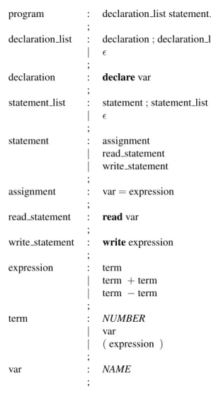
program : declaration list statement list ;
declaration list : declaration;declaration list
|
;
declaration : declarevar ;
statement list : statement;statement list
|
;
statement : assignment
| read statement
| write statement ;
assignment : var=expression ;
read statement : readvar ;
write statement : writeexpression ;
expression : term
| term +term
| term −term ;
term : NUMBER
| var
| (expression ) ;
var : NAME
;
Figure 1.2: The syntax of the Micro language
1.3.1
Micro
The syntax of Micro is described by the rules in Figure 1.2. We will see in Chap-ter 3 that such rules can be formalized into what is called agrammar.
Note that NUMBER and NAME have not been further defined. The idea is, of course, thatNUMBERrepresents a sequence of digits and thatNAMErepresents a string of letters and digits, starting with a letter.
A simple Micro program is shown in Figure 1.3
{
declare xyz; xyz = (33+3)-35; write xyz;
}
Figure 1.3: A Micro program
The semantics of Micro should be clear2: a Micro program consists of a sequence of read/write or assignment statements. There are integer-valued variables (which need to be declared before they are used) and expressions are restricted to addition and substraction.
1.3.2
x86 code
The target language will be code for the x86 processor family. Figure 1.4 shows part of the output of the compiler for the program of Figure 1.3. The full output can be found in Section B.6.2, page 157.
X86 processors have a number of registers, some of which are special purpose, such as theespregister which always points to the top of the stack (which grows downwards). More information on x86 assembler programming can be found in the Appendix, Section A, page 139.
line 1 The code is divided into data and text sections where the latter contains the actual instructions.
line 2 This defines a data area of 4 bytes wide which can be referenced using the namexyz. This definition is the translation of a Microdeclaration.
1 .section .data
2 .lcomm xyz, 4
3 .section .text
...
44 .globl main
45 .type main, @function
46 main:
47 pushl %ebp
48 movl %esp, %ebp
49 pushl $33
50 pushl $3
51 popl %eax
52 addl %eax, (%esp)
53 pushl $35
54 popl %eax
55 subl %eax, (%esp)
56 popl xyz
57 pushl xyz
58 call print
59 movl %ebp, %esp
60 popl %ebp
61 ret
...
Figure 1.4: X86 assembly code generated for the program in Figure 1.3
line 44 This defines main as a globally available name. It will be used to refer to the single function (line 45) that contains the instructions corresponding to the Micro program. The function starts at line 46 where the location corresponding to the label ’main’ is defined.
line 47 Together with line 48, this starts off the function according to the C call-ing conventions: the current top of stack contains the return address. This address has been pushed on the stack by the (function) call instruction. It will eventually be used (and popped) by a subsequent ret(return from function call) instruction. Parameters are passed by pushing them on the stack just before the call instruction. Line 47 saves the caller’s “base pointer” in theebpregister by pushing it on the stack before setting (line 48) the current top of the stack as a new base pointerebp. When returning from the function call, the orginal stack is restored by copying the saved value fromebptoesp(line 59) and popping the saved base pointer (line 60).
line 51 Once both operands are on the top of the stack, the operation (corresponding to the33 + 3expression) is executed by popping the second argument to the
eaxregister (line 51) which is then added to the first argument on the top of the stack (line 52). The net result is that the two arguments of the operation are replaced on the top of the stack by the (single) result of the operation.
line 53 To substract35from the result, this second argument of the substraction is pushed on the stack (line 53), after which the substraction is executed on the two operands on the stack, replacing them on the top of the stack by the result (lines 54,55).
line 56 The result of evaluating the expression is assigned to the variable xyz by popping it from the stack to the appropriate address.
line 57 In order to print the value at address xyz, it is first pushed on the stack as a parameter for a subsequent call (line 58) to aprint function (the code of which can be found in Section B.6.2).
1.3.3
Lexical analysis
The raw input to a compiler consists of a string of bytes or characters. Some of those characters, e.g. the “{” character in Micro, may have a meaning by themselves. Other characters only have meaning as part of a larger unit. E.g. the “y” in the example program from Figure 1.3, is just a part of the NAME “xyz”. Still others, such as “ ”, “\n” serve as separators to distinguish one meaningful string from another.
The first job of a compiler is then to group sequences of raw characters into mean-ingfultokens. The lexical analyzer module is responsible for this. Conceptually, the lexical analyzer (often called scanner) transforms a sequence of characters into a sequence of tokens. In addition, a lexical analyzer will typically access the symbol table to store and/or retrieve information on certain source language concepts such as variables, functions, types.
For the example program from Figure 1.3, the lexical analyzer will transform the character sequence
{ declare xyz; xyz = (33+3)-35; write xyz; }
into the token sequence shown in Figure 1.5.
Note that some tokens have “properties”, e.g. a hNUMBERi token has a value
hLBRACEi
hDECLARE symbol table ref=0i hNAME symbol table ref=3i hSEMICOLONi
hNAME symbol table ref=3i hASSIGNi
hLPARENi
hNUMBER value=33i hPLUSi
hNUMBER value=3i hRPARENi
hMINUSi
hNUMBER value=35i hSEMICOLONi
hWRITE symbol table ref=2i hNAME symbol table ref=3i hSEMICOLONi
hRBRACEi
Figure 1.5: Result of lexical analysis of program in Figure 1.3
After the scanner finishes, the symbol table in the example could look like
0 “declare” DECLARE 1 “read” READ 2 “write” WRITE 3 “xyz” NAME where the third column indicates the type of symbol.
Clearly, the main difficulty in writing a lexical analyzer will be to decide, while reading characters one by one, when a token of which type is finished. We will see in Chapter 2 that regular expressions and finite automata provide a powerful and convenient method to automate this job.
1.3.4
Syntax analysis
Once lexical analysis is finished, the parsertakes over to check whether the se-quence of tokens is grammatically correct, according to the rules that define the syntax of the source language.
Such matching can conveniently be represented as a parse tree. The parse tree corresponding to the token sequence of Figure 1.5 is shown in Figure 1.6.
<program> <statement> <statement_list> <statement> <RBRACE} <SEMICOLON> <SEMICOLON> <LBRACE> <statement_list> <assignment> <expression> <term> <term> <expression> <term> (xyz) <term> (33) (3) (35) <NAME> <ASSIGN> <MINUS>
<LPAREN> <RPAREN> <NUMBER>
<NUMBER> <PLUS> <NUMBER> <statement> <SEMICOLON> <write_statement> <expression> <term> <var> (xyz) <NAME> <WRITE> <declaration> (xyz) <DECLARE> <NAME> <statement_list> <>
Figure 1.6: Parse tree of program in Figure 1.3
Note that in the parse tree, a node and its children correspond to a rule in the syntax specification of Micro: the parent node corresponds to the left hand side of the rule while the children correspond to the right hand side. Furthermore, the yield3 of the parse tree is exactly the sequence of tokens that resulted from the
lexical analysis of the source text.
Hence the job of the parser is to construct a parse tree that fits, according to the syntax specification, the token sequence that was generated by the lexical ana-lyzer.
In Chapter 3, we’ll see how context-free grammars can be used to specify the syntax of a programming language and how it is possible to automatically generate parser programs from such a context-free grammar.
1.3.5
Semantic analysis
Having established that the source text is syntactically correct, the compiler may now perform additional checks such as determining the type of expressions and
checking that all statements are correct with respect to the typing rules, that vari-ables have been properly declared before they are used, that functions are called with the proper number of parameters etc.
This phase is carried out using information from the parse tree and the symbol ta-ble. In our example, very little needs to be checked, due to the extreme simplicity of the language. The only check that is performed verifies that a variable has been declared before it is used.
1.3.6
Intermediate code generation
In this phase, the compiler translates the source text into an simple intermediate language. There are several possible choices for an intermediate language. but in this example we will use the popular “three-address code” format. Essentially, three-address code consists of assignments where the right-hand side must be a single variable or constant or the result of a binary or unary operation. Hence an assignment involves at most three variables (addresses), which explains the name. In addition, three-address code supports primitive control flow statements such asgoto,branch-if-positiveetc. Finally, retrieval from and storing into a one-dimensional array is also possible.
The translation process issyntax-directed. This means that
• Nodes in the parse tree have a set of attributes that contain information pertaining to that node. The set of attributes of a node depends on the kind of syntactical concept it represents. E.g. in Micro, an attribute of an hexpressionicould be the sequence of x86 instructions that leave the result of the evaluation of the expression on the top of the stack. Similarly, both hvariandhexpressioninodes have anameattribute holding the name of the variable containing the current value of thehvariorhexpressioni
We usen.ato refer to the value of the attributeafor the noden.
• A number of semantic rules are associated with each syntactic rule of the grammar. These semantic rules determine the values of the attributes of the nodes in the parse tree (a parent node and its children) that correspond to such a syntactic rule. E.g. in Micro, there is a semantic rule that says that the code associated with anhassignmentiin the rule
consists of the code associated withhexpressionifollowed by a three-address code statement of the form
var.name =expression.name
More formally, such a semantic rule might be written as
assignment.code =expression.code k“var.name=expression.name”
• The translation of the source text then consists of the value of a particular attribute for the root of the parse tree.
Thus intermediate code generation can be performed by computing, using the semantic rules, the attribute values of all nodes in the parse tree. The result is then the value of a specific (e.g. “code”) attribute of the root of the parse tree.
For the example program from Figure 1.3, we could obtain the three-address code in Figure 1.7.
T0 = 33 +3 T1 = T0 - 35 XYZ = T1 WRITE XYZ
Figure 1.7: three-address code corresponding to the program of Figure 1.3
Note the introduction of several temporary variables, due to the restrictions in-herent in three-address code. The last statement before the WRITE may seem wasteful but this sort of inefficiency is easily taken care of by the next optimiza-tion phase.
1.3.7
Optimization
In this phase, the compiler tries several optimization methods to replace fragments of the intermediate code text with equivalent but faster (and usually also shorter) fragments.
Techniques that can be employed include common subexpression elimination, loop invariant motion, constant folding etc. Most of these techniques need ex-tra information such as a flow graph, live variable status etc.
XYZ = 1 WRITE XYZ
Figure 1.8: Optimized three-address code corresponding to the program of Fig-ure 1.3
1.3.8
Code generation
Lexical analysis
2.1
Introduction
As seen in Chapter 1, the lexical analyzer must transform a sequence of “raw” characters into a sequence oftokens. Often a token has a structure as in Figure 2.1.
1 #ifndef LEX_H 2 #define LEX_H
3 // %M%(%I%) %U% %E%
4
5 typedef enum { NAME, NUMBER, LBRACE, RBRACE, LPAREN, RPAREN, ASSIGN,
6 SEMICOLON, PLUS, MINUS, ERROR } TOKENT;
7
8 typedef struct
9 {
10 TOKENT type;
11 union {
12 int value; /* type == NUMBER */
13 char *name; /* type == NAME */
14 } info;
15 } TOKEN;
16
17 extern TOKEN *lex(); 18 #endif LEX_H
Figure 2.1: A declaration for TOKEN and lex()
Actually, the above declaration is not realistic. Usually, more “complex” tokens such as NAMEs will refer to a symbol table entry rather than simply their string representation.
Clearly, we can split up the scanner using a functionlex()as in Figure 2.1 which returns the next token from the source text.
It is not impossible1 to write such a function by hand. A simple implementation of a hand-made scanner for Micro (see Chapter 1 for a definition of “Micro”) is shown below.
1 // %M%(%I%) %U% %E%
2
3 #include <stdio.h> /* for getchar() and friends */
4 #include <ctype.h> /* for isalpha(), isdigit() and friends */
5 #include <stdlib.h> /* for atoi() */
6 #include <string.h> /* for strdup() */
7
8 #include "lex.h" 9
10 static int state = 0;
11
12 #define MAXBUF 256
13 static char buf[MAXBUF]; 14 static char* pbuf;
15
16 static char* token_name[] =
17 {
18 "NAME", "NUMBER", "LBRACE", "RBRACE", 19 "LPAREN", "RPAREN", "ASSIGN", "SEMICOLON",
20 "PLUS", "MINUS", "ERROR"
21 };
22
23 static TOKEN token; 24 /*
25 * This code is not robust: no checking on buffer overflow, ...
26 * Nor is it complete: keywords are not checked but lumped into
27 * the ’NAME’ token type, no installation in symbol table, ...
28 */
29 TOKEN* 30 lex() 31 {
32 char c; 33
34 while (1)
35 switch(state) 36 {
37 case 0: /* stands for one of 1,4,6,8,10,13,15,17,19,21,23 */
38 pbuf = buf;
39 c = getchar();
40 if (isspace(c))
41 state = 11;
42 else if (isdigit(c))
43 {
44 *pbuf++ = c; state = 2;
45 }
46 else if (isalpha(c))
47 {
48 *pbuf++ = c; state = 24;
49 }
50 else switch(c)
51 {
52 case ’{’: state = 5; break;
53 case ’}’: state = 7; break;
54 case ’(’: state = 9; break;
55 case ’)’: state = 14; break;
56 case ’+’: state = 16; break;
57 case ’-’: state = 18; break;
58 case ’=’: state = 20; break;
59 case ’;’: state = 22; break;
60 default:
61 state = 99; break;
62 }
63 break;
64 case 2:
65 c = getchar();
66 if (isdigit(c))
67 *pbuf++ = c;
68 else
69 state = 3;
70 break;
71 case 3:
72 token.info.value= atoi(buf);
73 token.type = NUMBER;
74 ungetc(c,stdin);
75 state = 0; return &token;
76 break;
77 case 5:
78 token.type = LBRACE;
79 state = 0; return &token;
80 break;
81 case 7:
82 token.type = RBRACE;
83 state = 0; return &token;
84 break;
85 case 9:
86 token.type = LPAREN;
87 state = 0; return &token;
88 break;
89 case 11:
91 if (isspace(c))
92 ;
93 else
94 state = 12;
95 break;
96 case 12:
97 ungetc(c,stdin);
98 state = 0;
99 break;
100 case 14:
101 token.type = RPAREN;
102 state = 0; return &token;
103 break;
104 case 16:
105 token.type = PLUS;
106 state = 0; return &token;
107 break;
108 case 18:
109 token.type = MINUS;
110 state = 0; return &token;
111 break;
112 case 20:
113 token.type = ASSIGN;
114 state = 0; return &token;
115 break;
116 case 22:
117 token.type = SEMICOLON;
118 state = 0; return &token;
119 break;
120 case 24:
121 c = getchar();
122 if (isalpha(c)||isdigit(c))
123 *pbuf++ = c;
124 else
125 state = 25;
126 break;
127 case 25:
128 *pbuf = (char)0;
129 token.info.name = strdup(buf);
130 token.type = NAME;
131 ungetc(c,stdin);
132 state = 0; return &token;
133 break;
134 case 99:
135 if (c==EOF)
136 return 0;
137 fprintf(stderr,"Illegal character: \’%c\’\n",c);
138 token.type = ERROR;
140 break;
141 default:
142 break; /* Cannot happen */
143 } 144 }
145 146 int
147 main() 148 {
149 TOKEN *t; 150
151 while ((t=lex())) 152 {
153 printf("%s",token_name[t->type]); 154 switch (t->type)
155 {
156 case NAME:
157 printf(": %s\n",t->info.name);
158 break;
159 case NUMBER:
160 printf(": %d\n",t->info.value);
161 break;
162 default:
163 printf("\n");
164 break;
165 } 166 }
167 return 0; 168 }
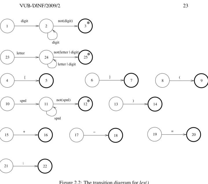
The control flow in the abovelex()procedure can be represented by a combination of so-called transition diagrams which are shown in Figure 2.2.
There is a transition diagram for each token type and another one for white space (blank, tab, newline). The code for lex() simply implements those diagrams. The only complications are
• When starting a new token (i.e., upon entry to lex()), we use a “special” state 0 to represent the fact that we didn’t decide yet which diagram to follow. The choice here is made on the basis of the next input character.
to-digit not(digit)
digit
letter
letter | digit not(letter | digit)
*
*
1 2 3
*
spnlspnl not(spnl)
} (
)
+ − =
;
16
21 22
15 17
10 11 12 13
18
14
19 20
9 8
7 6
{
5 4
23 24 25
Figure 2.2: The transition diagram forlex()
ken. In such a case we must push the extra character back onto the input before returning. Such states have been marked with a * in Figure 2.2.
• If we read a character that doesn’t fit any transition diagram, we return a specialERRORtoken type.
Clearly, writing a scanner by hand seems to be easy, once you have a set of tran-sition diagrams such as the ones in Figure 2.2. It is however also boring, and error-prone, especially if there are a large number of states.
Fortunately, the generation of such code can be automated. We will describe how a specification of the various token types can be automatically converted in code that implements a scanner for such token types.
2.2
Regular expressions
In Micro, a NUMBER token represents a digit followed by 0 or more digits. A
NAME consists of a letter followed by 0 or more alphanumeric characters. A
LBRACEtoken consists of exactly one “{” character, etc.
Such specifications are easily formalized usingregular expressions. Before defin-ing regular expressions we should recall the notion of alphabet (a finite set of abstract symbols, e.g. ASCII characters), and(formal) language(a set of strings containing symbols from some alphabet).
The length of a stringw, denoted|w|is defined as the number of symbols occur-ring inw. The prefix of lengthlof a stringw, denotedprefl(w)is defined as the longest stringxsuch that|x| ≤landw=xyfor some stringy. Theempty string
(of length 0) is denoted. TheproductL1.L2 of two languages is the language
L1.L2 ={xy |x∈L1 ∧ y ∈L2}
TheclosureL∗ of a languageLis defined by
L∗ =∪i∈NL i
(where, of course,L0 ={}andLi+1 =L.Li).
Definition 1 The following table, whererandsdenote arbitrary regular expres-sions, recursively defines all regular expressions over a given alphabetΣ, together with the languageLxeach expressionxrepresents.
Regular expression Language
∅ ∅
{}
a {a}
(r+s) Lr∪Ls
(rs) Lr·Ls
(r∗) L∗r
In the table, randsdenote arbitrary regular expressions, anda ∈ Σis an arbi-trary symbol fromΣ.
We assume that the operators+, concatenation and∗have increasing precedence, allowing us to drop many parentheses without risking confusion. Thus,((0(1∗)) + 0)
may be written as01∗+ 0.
From Figure 2.2 we can deduce regular expressions for each token type, as shown in Figure 2.1. We assume that
Σ ={a, . . . , z, A, . . . , Z,0, . . . ,9,SP,NL,(,),+,=,{,},;,−}
Token type or abbreviation Regular expression letter a+. . .+z+A+. . .+Z
digit 0 + 1 + 2 + 3 + 4 + 5 + 6 + 7 + 8 + 9
NUMBER digit(digit)∗
NAME letter(letter+digit)∗
space (SP+NL)(SP+NL)∗
LBRACE {
.. ..
Table 2.1: Regular expressions describing Micro tokens
A full specification, such as the one in Section B.1, page 149, then consists of a set of (extended) regular expressions, plus C code for each expression. The idea is that the generated scanner will
• Process input characters, trying to find a longest string that matches any of the regular expressions2.
• Execute the code associated with the selected regular expression. This code can, e.g. install something in the symbol table, return a token type or what-ever.
In the next section we will see how a regular expression can be converted to a so-calleddeterministic finite automatonthat can be regarded as an abstract machine to recognize strings described by regular expressions. Automatic translation of such an automaton to actual code will turn out to be straightforward.
2.3
Finite state automata
2.3.1
Deterministic finite automata
Definition 2 Adeterministic finite automaton(DFA) is a tuple
(Q,Σ, δ, q0, F)
where
• Qis a finite set ofstates,
• Σis a finiteinput alphabet
• δ :Q×Σ→Qis a (total) transition function
• q0 ∈Qis theinitial state
• F ⊆Qis the set offinal states
Definition 3 LetM = (Q,Σ, δ, q0, F)be a DFA. Aconfiguration ofM is a pair (q, w)∈Q×Σ∗. For a configuration(q, aw)(wherea∈Σ), we write
(q, aw)`M (q0, w)
just whenδ(q, a) =q0 3. The reflexive and transitive closure of the binary relation
`M is denoted as`∗M. A sequence
c0 `M c1 `M . . .`M cn
is called acomputationofn ≥0steps byM.
Thelanguage accepted byM is defined by
L(M) ={w| ∃q ∈F ·(q0, w)`∗M (q, )}
We will often write δ∗(q, w) to denote the unique q0 ∈ Q such that (q, w) `∗ M (q0, ).
3We will drop the subscriptM in`
Example 1 Assuming an alphabet Σ = {l, d, o} (where “l” stands for “letter”, “d” stands for “digit” and “o” stands for “other”), a DFA recognizing Micro
NAMEs can be defined as follows:
M = ({q0, qe, q1},{l, d, o}, δ, q0,{q1})
whereδis defined by
δ(q0, l) = q1 δ(q0, d) = qe δ(q0, o) = qe δ(q1, l) = q1
δ(q1, d) = q1 δ(q1, o) = qe δ(qe, l) = qe δ(qe, d) = qe δ(qe, o) = qe
M is shown in Figure 2.3 (the initial state has a small incoming arrow, final states are in bold):
q0 q1
qe l
l d o
o d l d
o
Figure 2.3: A DFA forNAME
Clearly, a DFA can be efficiently implemented, e.g. by encoding the states as numbers and using an array to represent the transition function. This is illustrated in Figure 2.4. The next statearray can be automatically generated from the DFA description.
1 typedef int STATE; 2 typedef char SYMBOL;
3 typedef enum {false,true} BOOL; 4
5 STATE next_state[SYMBOL][STATE];
6 BOOL final[STATE];
7
8 BOOL
9 dfa(SYMBOL *input,STATE q) 10 {
11 SYMBOl c; 12
13 while (c=*input++)
14 q = next_state[c,q];
15 return final[q]; 16 }
Figure 2.4: DFA implementation
2.3.2
Nondeterministic finite automata
Anondeterministic finite automatonis much like a deterministic one except that we now allow several possibilities for a transition on the same symbol from a given state. The idea is that the automaton can arbitrarily (nondeterministically) choose one of the possibilities. In addition, we will also allow-moveswhere the automaton makes a state transition (labeled by) without reading an input symbol.
Definition 4 Anondeterministic finite automaton(NFA) is a tuple
(Q,Σ, δ, q0, F)
where
• Qis a finite set ofstates,
• Σis a finiteinput alphabet
• δ :Q×(Σ∪ {})→2Q is a (total) transition function4
• q0 ∈Qis theinitial state
b
a
q
2q
1q
0a
b
Figure 2.5:M1
It should be noted that ∅ ∈ 2Q and thus Definition 4 sanctions the possibility of there not being any transition from a stateqon a given symbola.
Example 2 Consider M1 = ({q0, q1, q2}, δ1, q0,{q0}) as depicted in Figure 2.5.
The table below definesδ1:
q ∈Q σ ∈Σ δ1(q, σ)
q0 a {q1}
q0 b ∅
q1 a ∅
q1 b {q0, q2} q2 a {q0}
q2 b ∅
The following definition formalizes our intuition about the behavior of nondeter-ministic finite automata.
Definition 5 LetM = (Q,Σ, δ, q0, F)be a NFA. AconfigurationofM is a pair (q, w)∈Q×Σ∗. For a configuration(q, aw)(wherea∈Σ∪ {}), we write
(q, aw)`M (q0, w)
just whenq0 ∈δ(q, a)5. The reflexive and transitive closure of the binary relation
`M is denoted as`∗M. Thelanguage accepted byM is defined by
L(M) ={w| ∃q ∈F ·(q0, w)`∗M (q, )}
4For any setX, we use2Xto denote its power set, i.e. the set of all subsets ofX.
5We will drop the subscriptM in`
Example 3 The following sequence shows howM1 from Example 2 can accept
the stringabaab:
(q0, abaab) `M1 (q1, baab)
`M1 (q2, aab)
`M1 (q0, ab)
`M1 (q1, b)
`M1 (q0, )
L(M1) = {w0w1. . . wn |n∈N∧ ∀0≤i≤n·wi ∈ {ab, aba}}
Although nondeterministic finite automata are more general than deterministic ones, it turns out that they are not more powerful in the sense that any NFA can be simulated by a DFA.
Theorem 1 LetM be a NFA. There exists a DFAM0such thatL(M0) =L(M).
Proof: (sketch) LetM = (Q,Σ, δ, q0, F)be a NFA. We will construct a DFAM0
that simulates M. This is achieved by letting M0 be “in all possible states” that
M could be in (after reading the same symbols). Note that “all possible states” is always an element of2Q, which is finite sinceQis.
To deal with -moves, we note that, ifM is in a state q, it could also be in any state q0 to which there is an -transition fromq. This motivates the definition of the-closureC(S)of a set of statesS:
C(S) = {p∈Q| ∃q ∈S·(q, )`∗M (p, )} (2.1)
Now we define
M0 = (2Q,Σ, δ0, s0, F0)
where
• δ0is defined by
∀s∈2Q, a∈Σ·δ0(s, a) = ∪q∈sC(δ(q, a)) (2.2)
• s0 =C(q0), i.e. M0 starts in all possible states whereM could go to from q0 without reading any input.
• F0 ={s∈2Q |s∩F 6=∅}, i.e. ifM couldend up in a final state, thenM0
willdo so.
2.4
Regular expressions vs finite state automata
In this section we show how a regular expression can be translated to a nondeter-ministic finite automata that defines the same language. Using Theorem 1, we can then translate regular expressions to DFA’s and hence to a program that accepts exactly the strings conforming to the regular expression.
Theorem 2 Letrbe a regular expression. Then there exists a NFAMr such that L(Mr) =Lr.
Proof:
We show by induction on the number of operators used in a regular expression r
thatLris accepted by an NFA
Mr = (Q,Σ, δ, q0,{qf})
(whereΣis the alphabet ofLr) which has exactly one final stateqf satisfying
∀a∈Σ∪ {} ·δ(qf, a) =∅ (2.3)
Base case
Assume thatrdoes not contain any operator. Thenris one of∅,ora∈Σ.
We then defineM∅,MandMaas shown in Figure 2.6.
a
M
aM
M
∅Figure 2.6:M∅, MandMa
Induction step
More complex regular expressions must be of one of the formsr1+r2,r1r2orr1∗.
M
r1∗M
r1r2M
r1+r2M
r1M
r2q
0q
fq
0q
fM
r1q
0q
fM
r2M
r1Figure 2.7: Mr1+r2, Mr1r2 andMr1∗
It can then be shown that
L(Mr1+r2) = L(Mr1)∪L(Mr2) L(Mr1r2) = L(Mr1)L(Mr2)
L(Mr∗1) = L(Mr1) ∗
2
2.5
A scanner generator
We can now be more specific on the design and operation of a scanner generator such aslex(1)orflex(1L), which was sketched on page 25.
First we introduce the concept of a “dead” state in a DFA.
Definition 6 LetM = (Q,Σ, δ, q0, F)be a DFA. A stateq ∈ Qis calleddeadif there does not exist a stringw∈Σ∗ such that(q, w)`∗
Example 4 The stateqein Example 1 is dead.
It is easy to determine the set of dead states for a DFA, e.g. using a marking algorithm which initially marks all states as “dead” and then recursively works backwards from the final states, unmarking any states reached.
The generator takes as input a set of regular expressions,R ={r1, . . . , rn}each of
which is associated with some codecrito be executed when a token corresponding
toriis recognized.
The generator will convert the regular expression
r1+r2+. . .+rn
to a DFAM = (Q,Σ, δ, q0, F), as shown in Section 2.4, with one addition: when
constructingM, it will remember which final state of the DFA corresponds with which regular expression. This can easily be done by remembering the final states in the NFA’s corresponding to each of theriwhile constructing the combined DFA M. It may be that a final state in the DFA corresponds to several patterns (regular expressions). In this case, we select the one that was defined first.
Thus we have a mapping
pattern:F →R
which associates the first (in the order of definition) pattern to which a certain final state corresponds. We also compute the set of dead states ofM.
The code in Figure 2.8 illustrates the operation of the generated scanner.
1 typedef int STATE; 2 typedef char SYMBOL;
3 typedef enum {false,true} BOOL; 4
5 typedef struct { /* what we need to know about a user defined pattern */
6 TOKEN* (*code)(); /* user-defined action */
7 BOOL do_return; /* whether action returns from lex() or not */
8 } PATTERN;
9
10 static STATE next_state[SYMBOL][STATE]; 11 static BOOL dead[STATE];
12 static BOOL final[STATE];
13 static PATTERN* pattern[STATE]; /* first regexp for this final state */
14 static SYMBOL *last_input = 0; /* input pointer at last final state */
15 static STATE last_state, q = 0; /* assuming 0 is initial state */
16 static SYMBOL *input; /* source text */
17
18 TOKEN* 19 lex() 20 {
21 SYMBOl c;
22 PATTERN *last_pattern = 0; 23
24 while (c=*input++) {
25 q = next_state[c,q];
26 if (final[q]) {
27 last_pattern = pattern[q];
28 last_input = input;
29 last_state = q;
30 }
31 if (dead[q]) {
32 if (last_pattern) {
33 input = last_input;
34 q = 0;
35 if (last_pattern->do_return)
36 return pattern->code();
37 else
38 pattern->code();
39 }
40 else /* error */
41 ;
42 }
43 } 44
45 return (TOKEN*)0;
46 }
Parsing
3.1
Context-free grammars
As mentioned in Section 1.3.1, page 9, the rules (or railroad diagrams) used to specify the syntax of a programming language can be formalized using the concept of context-free grammar.
Definition 7 Acontext-free grammar(cfg) is a tuple
G= (V,Σ, P, S)
where
• V is a finite set ofnonterminalsymbols
• Σis a finite set ofterminalsymbols, disjoint fromV: Σ∩V =∅.
• P is a finite set of productions of the form A → α where A ∈ V and
α∈(V ∪Σ)∗
• S ∈V is a nonterminalstart symbol
Note that terminal symbols correspond to token types as delivered by the lexical analyzer.
Example 5 The following context-free grammar defines the syntax of simple arithmetic expressions:
G0 = ({E},{+,×,(,),id}, P, E)
whereP consists of
E → E+E E → E×E E → (E) E → id
We shall often use a shorter notation for a set of productions where several right-hand sides for the same nonterminal are written together, separated by “|”. Using this notation, the set of rules ofG0 can be written as
E →E+E | E×E | (E) | id
Definition 8 LetG= (V,Σ, P, S)be a context-free grammar. For stringsx, y ∈(V ∪Σ)∗, we say thatxderivesyin one step, denotedx=⇒G yiffx=x1Ax2,y=x1αx2
andA→α∈P. Thus=⇒Gis a binary relation on(V ∪Σ)∗. The relation=⇒∗G is the reflexive and transitive closure of=⇒G. ThelanguageL(G)generated by Gis defined by
L(G) ={w∈Σ∗ |S =⇒∗ G w}
A language is calledcontext-freeif it is generated by some context-free grammar.
AderivationinGofwnfromw0is any sequence of the form
w0 =⇒Gw1 =⇒G. . .=⇒G wn
wheren≥0(we say that the derivation hasnsteps) and∀1≤i≤n·wi ∈(V ∪Σ)∗ We writev =⇒n
Gw(n≥0) whenwcan be derived fromvinnsteps.
Thus a context-free grammar specifies precisely which sequences of tokens are valid sentences (programs) in the language.
Example 6 Consider the grammarG0from Example 5. The following is a
deriva-tion inGwhere at each step, the symbol to be rewritten is underlined.
S =⇒G0 E×E
=⇒G0 (E)×E
=⇒G0 (E+E)×E
A derivation in a context-free grammar is conveniently represented by a parse tree.
Definition 9 LetG = (V,Σ, P, S)be a context-free grammar. Aparse tree cor-responding to G is a labeled tree where each node is labeled by a symbol from
V ∪Σin such a way that, ifAis the label of a node andA1A2. . . An(n >0) are the labels of its children (in left-to-right order), then
A→A1A1. . . An
is a rule inP. Note that a ruleA →gives rise to a leaf node labeled.
As mentioned in Section 1.3.4, it is the job of the parser to convert a string of tokens into a parse tree that has precisely this string as yield. The idea is that the parse tree describes the syntactical structure of the source text.
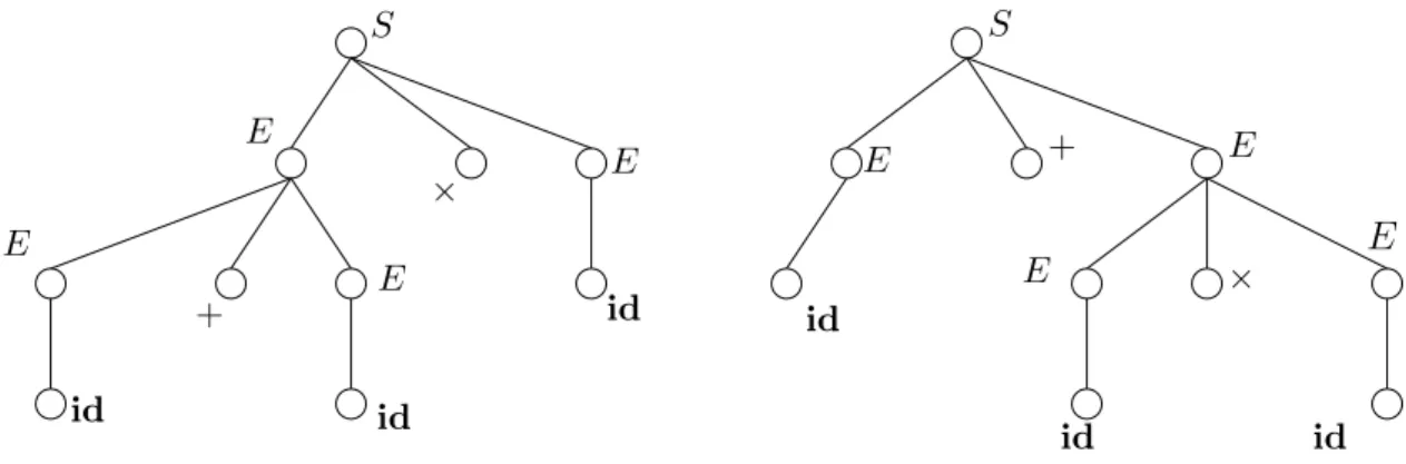
However, sometimes, there are several parse trees possible for a single string of tokens, as can be seen in Figure 3.1.
E
E
S
E
E
id id
id
S
+
E E
E ×
E
id id
id ×
+
Figure 3.1: Parse trees in the ambiguous context-free grammar from Example 5
Note that the two parse trees intuitively correspond to two evaluation strategies for the expression. Clearly, we do not want a source language that is specified using an ambiguous grammar (that is, a grammar where a legal string of tokens may have different parse trees).
Example 7 Fortunately, we can fix the grammar from Example 5 to avoid such ambiguities.
whereP0 consists of
E → E+T | T
T → T ×F | F F → (E) | id
is an unambiguous grammar generating the same language as the grammar from Example 5.
Still, there are context-free languages such as{aibjck|i=j∨j =k}for which only ambiguous grammars can be given. Such languages are called inherently ambiguous. Worse still, checking whether an arbitrary context-free grammar al-lows ambiguity is an unsolvable problem[HU69].
3.2
Top-down parsing
3.2.1
Introduction
When using a top-down (also called predictive) parsing method, the parser tries to find aleftmost derivation (and associated parse tree) of the source text. A left-most derivation is a derivation where, during each step, the leftleft-most nonterminal symbol is rewritten.
Definition 10 LetG= (V,Σ, P, S)be a context-free grammar. For stringsx, y ∈
(V ∪Σ)∗, we say thatxderivesyin a leftmost fashion and in one step, denoted
x=L⇒G y
iffx = x1Ax2, y = x1αx2,A → αis a rule inP andx1 ∈ Σ∗ (i.e. the leftmost occurrence of a nonterminal symbol is rewritten).
The relation L =⇒∗
Gis the reflexive and transitive closure of L
=⇒G. A derivation
y0 L =⇒Gy1
L =⇒G. . .
L =⇒G yn
is called aleftmostderivation. Ify0 = S (the start symbol) then we call eachyi in such a derivation aleft sentential form.
S
c
d c a d
A
a b
S c a d
c a d
TryS →cAd
Matchc: OK. TryA→abforA. S
c
A d
Matcha: OK.
a b
Try next predicted symbolbin tree.
No match: BACKTRACK. Try next ruleA →aforA. S
c
d c a d
A
Matcha: OK.
Try next predicted symboldin tree. S
c
d c a d
A a
S
c
d c a d
A a
Matchd: OK. Parse succeeded.
Figure 3.2: A simple top-down parse
Theorem 3 LetG= (V,Σ, P, S)be a context-free grammar. IfA∈V ∪Σthen
A=⇒∗Gw∈Σ∗ iff A L
=⇒∗G w∈Σ∗
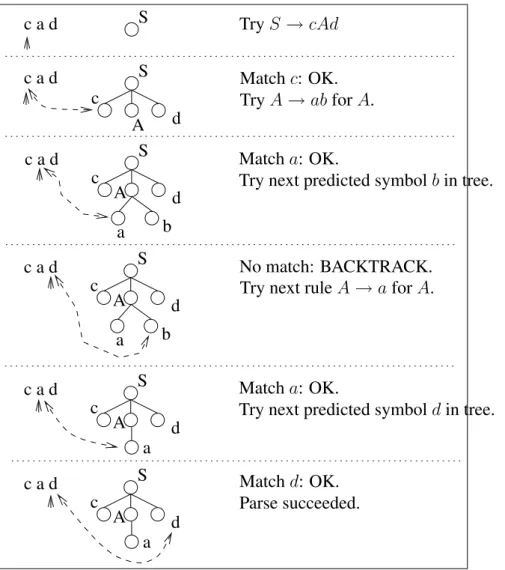
Example 8 Consider the trivial grammar
G= ({S, A},{a, b, c, d}, P, S)
whereP contains the rules
Let w = cad be the source text. Figure 3.2 shows how a top-down parse could proceed.
The reasoning in Example 8 can be encoded as shown below.
1 typedef enum {false,true} BOOL; 2
3 TOKEN* input; /* output array from scanner */
4 TOKEN* token; /* current token from input */
5
6 BOOL
7 parse_S() { /* Parse something derived from S */
8 /* Try rule S --> c A d */
9 if (*token==’c’) {
10 ++token;
11 if (parse_A()) {
12 if (*token==’d’) {
13 ++token;
14 return true;
15 } 16 } 17 }
18 return false; 19 }
20
21 BOOL
22 parse_A() { /* Parse stuff derived from A */
23 TOKEN* save; /* for backtracking */
24
25 save = token;
26
27 /* Try rule A --> a b */
28 if (*token==’a’) {
29 ++token;
30 if (*token==’b’) {
31 ++token;
32 return true;
33 } 34 } 35
36 token = save; /* didn’t work: backtrack */
37
38 /* Try rule A --> a */
39 if (*token==’a’) {
40 ++token;
41 return true; 42 }
43
45
46 /* no more rules: give up */
47 return false; 48 }
Note that the above strategy may need recursive functions. E.g. if the grammar contains a rule such as
E →(E)
the code forparse E()will contain a call toparse E().
The method illustrated above has two important drawbacks:
• It cannot be applied if the grammarGis left-recursive, i.e.A L =⇒∗
G Axfor
somex∈(V ∪Σ)∗.
Indeed, even for a “natural” rule such as
E →E+E
it is clear that the parse E() function would start by calling itself (in an infinite recursion), before reading any input.
We will see that it is possible to eliminate left recursion from a grammar without changing the generated language.
• Using backtracking is both expensive and difficult. It is difficult because it usually does not suffice to simply restore the input pointer: all actions taken by the compiler since the backtrack point (e.g. symbol table updates) must also be undone.
The solution will be to apply top-down parsing only for a certain class of restricted grammars for which it can be shown that backtracking will never be necessary.
3.2.2
Eliminating left recursion in a grammar
First we look at the elimination of immediateleft recursion where we have rules of the form
A→Aα | β
whereβdoes not start withA.
The idea is to reorganize the rules in such a way that derivations are simulated as shown in Figure 3.3
A A
A α
α
β
A
A0
A0 β
α
α
With left recursion Without left recursion
Figure 3.3: Eliminating immediate left recursion
Algorithm 1 [Removing immediate left recursion for a nonterminalAfrom a grammarG= (V,Σ, P, S)]
Let
A→Aα1 | . . . | Aαm | β1 | . . . | βn
be all the rules with A as the left hand side. Note that m > 0 and n ≥ 0and
∀0≤i≤n·βi 6∈A(V ∪Σ)∗
1. Ifn = 0, no terminal string can ever be derived fromA, so we may as well remove allA-rules.
2. Otherwise, define a new nonterminalA0, and replace theArules by
A → β1A0 | . . . | βnA0 A0 → α1A0 | . . . | αmA0 |
2
Example 9 Consider the grammar G1 from Example 7. Applying Algorithm 1
results in the grammar G2 = ({E, E0, T, T0, F},{+,×,(,),id}, PG2, E) where PG2 contains
E → T E0 E0 → +T E0 |
T → F T0 T0 → ×F T0 |
F → (E) | id
3.2.3
Avoiding backtracking: LL(1) grammars
When inspecting Example 8, it appears that in order to avoid backtracking, one should be able to predict with certainty, given the nonterminal X of the current functionparse X()and the next input tokena, which productionX →xwas used as a first step to derive a string of tokens that starts with the input tokenafromX.
The problem is graphically represented in Figure 3.4
a
S
X
x
Figure 3.4: The prediction problem
The following definition defines exactly the class of context-free grammars for which this is possible.
Definition 11 An LL(1) grammar is a context-free grammar G = (V,Σ, P, S)
such that if
S L
=⇒∗G w1Xx3 L
=⇒Gw1x2x3 L
=⇒∗Gw1aw4
and
S L
=⇒∗G w1Xxˆ3 L
=⇒Gw1xˆ2xˆ3 L
=⇒∗Gw1awˆ4
wherea∈Σ,X ∈V,w1 ∈Σ∗,w4 ∈Σ∗,wˆ4 ∈Σ∗then
x2 = ˆx2
Intuitively, Definition 11 just says that if there are two possible choices for a pro-duction, these choices are identical.
Thus for LL(1) grammars1, we know for sure that we can write functions as we did in Example 8, without having to backtrack. In the next section, we will see how to automatically generate parsers based on the same principle but without the overhead of (possibly recursive) function calls.
3.2.4
Predictive parsers
Predictive parsers use a stack (representing strings in(V ∪Σ)∗) and a parse table as shown in Figure 3.5.
w a
input
+ b $
Z
X Y
stack
PREDICTIVE PARSER
parse table $
V ×Σ→P ∪ {error}
Figure 3.5: A predictive parser
The figure shows the parser simulating a leftmost derivation
S =L⇒G . . . L
=⇒G wZY X
| {z }
depicted position of parser
L =⇒G . . .
L
=⇒Gwa+b
Note that the string consisting of the input read so far, followed by the contents of the stack (from the top down) constitutes a left sentential form. End markers (depicted as $ symbols) are used to mark both the bottom of the stack and the end of the input.
The parse tableM represents the production to be chosen: when the parser hasX
on the top of the stack andaas the next input symbol,M[X, a]determines which production was used as a first step to derive a string starting withafromX.
Algorithm 2 [Operation of an LL(1) parser]
The operation of the parser is shown in Figure 3.6. 2
Intuitively, a predictive parser simulates a leftmost derivation of its input, using the stack to store the part of the left sentential form that has not yet been processed (this part includes all nonterminals of the left sentential form). It is not difficult to see that if a predictive parser successfully processes an input string, then this string is indeed in the language generated by the grammar consisting of all the rules in the parse table.
To see the reverse, we need to know just how the parse table is constructed.
First we need some auxiliary concepts:
Definition 12 LetG= (V,Σ, P, S)be a context-free grammar.
• The functionfirst: (V ∪Σ)∗ →2(Σ∪{})is defined by
first(α) ={a|α=⇒∗G aw∈Σ∗} ∪Xα
where
Xα =
{} ifα=⇒∗ G
∅ otherwise
• The functionfollow:V →2(Σ∪{$}) is defined by
follow(A) = {a∈Σ|S =⇒∗GαAaβ} ∪Yα
where
Yα =
{$} ifS =⇒∗ GαA
∅ otherwise
Intuitively, first(α) contains the set of terminal symbols that can appear at the start of a (terminal) string derived from α, including ifαcan derive the empty string.
On the other hand,follow(A)consists of those terminal symbols that may follow a string derived fromAin a terminal string fromL(G).
1 PRODUCTION* parse_table[NONTERMINAL,TOKEN]; 2 SYMBOL End, S; /* marker and start symbol */
3 SYMBOL* stack;
4 SYMBOL* top_of_stack; 5
6 TOKEN *input; 7
8 BOOL
9 parse() { /* LL(1) predictive parser */
10 SYMBOL X;
11 push(End); push(S); 12
13 while (*top_of_stack!=End) {
14 X = *top_of_stack;
15 if (is_terminal(X)) {
16 if (X==*input) { /* predicted outcome */
17 ++input; /* advance input */
18 pop(); /* pop X from stack */
19 } 20 else
21 error("Expected %s, got %s", X, *input); 22 }
23 else { /* X is nonterminal */
24 PRODUCTION* p = parse_table[X,*input];
25 if (p) {
26 pop(); /* pop X from stack */
27 for (i=length_rhs(p)-1;(i>=0);--i)
28 push(p->rhs[i]); /* push symbols of rhs, last first */
29 } 30 else
31 error("Unexpected %s", *input); 32 }
33 }
34 if (*input==End)
35 return true; 36 else
37 error("Redundant input: %s", *input); 38 }
Figure 3.6: Predictive parser operation
Algorithm 3 [Construction of LL(1) parse table]
LetG= (V,Σ, P, S)be a context-free grammar.
1. Initialize the table:∀A∈V, b∈Σ·M[A, b] =∅
(a) For eachb ∈first(α)∩Σ, addA→αtoM[A, b].
(b) If∈first(α)then
i. For eachc∈follow(A)∩Σ, addA→αtoM[A, c].
ii. If$∈follow(A)then addA→αtoM[A,$].
3. If each entry inM contains at most a single production then return success, else return failure.
2
It can be shown that, if the parse table for a grammar G was successfully con-structed using Algorithm 3, then the parser of Algorithm 2 accepts exactly the strings ofL(G). Also, if Algorithm 3 fails, thenGis not an LL(1) grammar.
Example 10 Consider grammar G2 from Example 9. The firstandfollow
func-tions are computed in Examples 11 and 12. The results are summarized below.
E E0 T T0 F
first (,id +, (,id ×, (,id
follow $,) $,) +,$,) $,),+ ×,$,),+
Applying Algorithm 3 yields the following LL(1) parse table.
E E0 T T0 F
id E →T E0 T →F T0 F →id
+ E0 →+T E0 T0 →
× T0 → ×F T0
( E →T E0 T →F T0 F →(E)
) E0 → T0 →
$ E0 → T0 →
the input stringid+id×id.
stack input rule
$E id+id×id$
$E0T id+id×id$ E →T E0
$E0T0F id+id×id$ T →F T0
$E0T0id id+id×id$ F →id
$E0T0 +id×id$
$E0 +id×id$ T0 →
$E0T+ +id×id$ E0 →+T E0
$E0T id×id$
$E0T0F id×id$ T →F T0
$E0T0id id×id$ F →id
$E0T0 ×id$
$E0T0F× ×id$ T0 → ×F T0
$E0T0F id$
$E0T0id id$ F →id
$E0T0 $
$E0 $ T0 →
$ $ E0 →
3.2.5
Construction of first and follow
Algorithm 4 [Construction of first]
LetG= (V,Σ, P, S)be a context-free grammar. We construct an arrayF :V ∪Σ→2(Σ∪{})
and then show a function to computefirst(α)for arbitraryα∈(V ∪Σ)∗.
1. F is constructed via a fixpoint computation:
(a) for eachX ∈V, initializeF[X]← {a|X →aα, a∈Σ}
(b) for eacha ∈Σ, initializeF[a]← {a}
2. repeat the following steps
(a) F0 ←F
(b) for each ruleX →, addtoF[X].
(c) for each ruleX →Y1. . . Yk(k >0) do
i. for each1≤i≤ksuch thatY1. . . Yi−1 ∈V∗and∀1≤j < i·∈F[Yj] doF[X]←F[X]∪(F[Yi]\ {})
untilF0 =F
Define
first(X1. . . Xn) = S
1≤j≤(k+1)(F[Xj]\ {}) ifk(X1. . . Xn)< n S
1≤j≤nF[Xj]∪ {}) ifk(X1. . . Xn) =n
wherek(X1. . . Xn)is the largest indexk such thatX1. . . Xk =⇒∗G , i.e.
k(X1. . . Xn) = max{1≤i≤n | ∀1≤j ≤i·∈F[Xj}
2
Example 11 Consider grammarG2from Example 9.
The construction ofF is illustrated in the following table.
E E0 T T0 F
+ × (,id initialization
ruleE0 →
(,id ruleT →F T0
ruleT0 →
(,id ruleE →T E0
(,id +, (,id ×, (,id
Algorithm 5 [Construction of follow]
LetG= (V,Σ, P, S)be a context-free grammar. Thefollowset of all symbols in
V can be computed as follows:
1. follow(S)←$
2. Apply the following rules until nothing can be added tofollow(A)for any
A∈V.
(a) If there is a productionA→αBβ inP then
follow(B)←follow(B)∪(first(β)\ {})
(b) If there is a production A → αB or a production A → αBβ where
∈first(β)thenfollow(B)←follow(B)∪follow(A).
Example 12 Consider again grammarG2from Example 9.
The construction offollowis illustrated in the following table.
E E0 T T0 F
$ initialization
+ ruleE →T E0
) ruleF →(E)
× ruleT →F T0
$,) ruleE →T E0
$,) ruleE →T E0
$,),+ ruleT →F T0
$,),+ ruleT →F T0
$,) $,) +,$,) $,),+ ×,$,),+
3.3
Bottom-up parsing
3.3.1
Shift-reduce parsers
As described in Section 3.2, a top-down parser simulates a leftmost derivation in a top-down fashion. This simulation predicts the next production to be used, based on the nonterminal to be rewritten and the next input symbol.
A bottom-up parser simulates a rightmost derivation in a bottom-up fashion, where a rightmost derivation is defined as follows.
Definition 13 LetG= (V,Σ, P, S)be a context-free grammar. For stringsx, y ∈(V ∪Σ)∗, we say thatxderivesyin a rightmost fashion and in one step, denoted
x=R⇒G y
iffx=x1Ax2, y=x1αx2,A →αis a rule inP andx2 ∈Σ∗ (i.e. the rightmost occurrence of a nonterminal symbol is rewritten).
The relation R =⇒∗
Gis the reflexive and transitive closure of R
=⇒G. A derivation
x0 R =⇒G x1
R =⇒G . . .
R =⇒G xn
A phraseof a right sentential form is a sequence of symbols that have been de-rived from a single nonterminal symbol occurrence (in an earlier right sentential form of the derivation). A simple phrase is a phrase that contains no smaller phrase. Thehandleof a right sentential form is its leftmost simple phrase (which is unique). A prefix of a right sentential form that does not extend past its handle is called aviable prefixofG.
Example 13 Consider the grammar
G3 = ({S, E, T, F},{+,×,(,),id}, PG3, S)
wherePG3 consists of
S → E
E → E+T | T T → T ×F | F F → (E) | id
G3 is simply G1 from Example 7, augmented by a new start symbol whose only
use is at the left hand side of a single production that has the old start symbol as its right hand side.
The following table shows a rightmost derivation ofid+id×id; where the handle in each right sentential form is underlined.
S E E+T E+T ×F E+T ×id E+F ×id E+id×id T +id×id F +id×id id+id×id
Example 14 The table below illustrates the operation of a shift-reduce parser to simulate the rightmost derivation from Example 13. Note that the parsing has to be read from the bottom to the top of the figure and that both the stack and the input contain the end marker “$”.
derivation stack input operation
S $S $ accept
E $E $ reduceS →E
E+T $E+T $ reduceE →E+T
E+T ×F $E+T ×F $ reduceT →T ×F
$E+T ×id $ reduceF →id
$E+T× id$ shift
E+T ×id $E+T ×id$ shift
E+F ×id $E+F ×id$ reduceT →F $E+id ×id$ reduceF →id
$E+ id×id$ shift
E+id×id $E +id×id$ shift
T +id×id $T +id×id$ reduceE →T F +id×id $F +id×id$ reduceT →F $id +id×id$ reduceF →id id+id×id $ id+id×id$ shift
Clearly, the main problem when designing a shift-reduce parser is to decide when to shift and when to reduce. Specifically, the parser should reduce only when the handle is on the top of the stack. Put in another way, the stack should always contain aviable prefix.
We will see in Section 3.3.2 that the language of all viable prefixes of a context-free grammarGis regular, and thus there exists a DFAMG = (Q, V ∪Σ, δ, q0, F)
accepting exactly the viable prefixes ofG. The operation of a shift-reduce parser is outlined in Figure 3.72.
However, rather than checking each time the contents of the stack (and the next input symbol) vs. the DFAMG, it is more efficient to store the states together with
the symbols on the stack in such a way that for each prefix xX of (the contents of) the stack, we store the stateδ∗(q0, xX)together withX on the stack.
In this way, we can simply checkδMG(q, a)whereq ∈Qis the state on the top of
the stack andais the current input symbol, to find out whether shifting the input would still yield a viable prefix on the stack. Similarly, upon a reduce(A → α)
1 while (true) {
2 if ((the top of the stack contains the start symbol) && 3 (the current input symbol is the endmarker ’$’))
4 accept;
5 else if (the contents of the stack concatenated with the next
6 input symbol is a viable prefix)
7 shift the input onto the top of the stack; 8 else
9 if (there is an appropriate producion)
10 reduce by this production;
11 else
12 error;
13 }
Figure 3.7: Naive shift-reduce parsing procedure
operation, both A and δ(q, A) are pushed whereq is the state on the top of the stack after poppingα.
In practice, a shift-reduce parser is driven by two tables:
• An action table that associates a pair consisting of a state q ∈ Q and a symbol a ∈ Σ (the input symbol) with an action of one of the following types:
– accept, indicating that the parse finished successfully
– shift(q0), where q ∈ Q is a final state of MG. This action tells the
parser to push both the input symbol andqon top of the stack. In this caseδMG(q, a) =q0.
– reduce(A → α) where A → α is a production from G. This in-structs the parser to pop α (and associated states) from the top of the stack, then pushingA and the state q0 given byq0 = goto(q00, A)
whereq00is the state left on the top of the stack after poppingα. Here
goto(q00, A) =δMG(q00, A).
– error, indicating thatδMG(q, a)yields a dead state.
• Agototable:
goto :Q×V →Q
which is used during a reduce operation.
The architecture of a shift-reduce parser is shown in Figure 3.8.
input
$
$ E
+ T
×
+ id
id
q0 q1 q2 q3
q4 goto: V ×Q→Q
stack
SHIFT-REDUCE PARSER
id
×
action :Q×Σ→ACTION
Figure 3.8: A shift-reduce parser
Algorithm 6 [Shift-reduce parsing]
See Figure 3.9 on page 55. 2
3.3.2
LR(1) parsing
Definition 14 LetG= (V,Σ, P, S0)be a context-free grammar such thatS0 →S
is the only production forS0andS0 does not appear on the right hand side of any production.
• AnLR(1) itemis a pair[A →α•β, a]whereA →αβ is a production from
P,•is a new symbol anda ∈Σ∪ {$}is a terminal or end marker symbol. We useitemsGto denote the set of all items ofG.
• TheLR(1) viable prefix NFAofGis
NG= (itemsG, V ∪Σ, δ,[S0 → •S],itemsG)
whereδis defined by
[A→αX•β, a] ∈ δ([A→α•Xβ, a], X) for allX ∈V ∪Σ
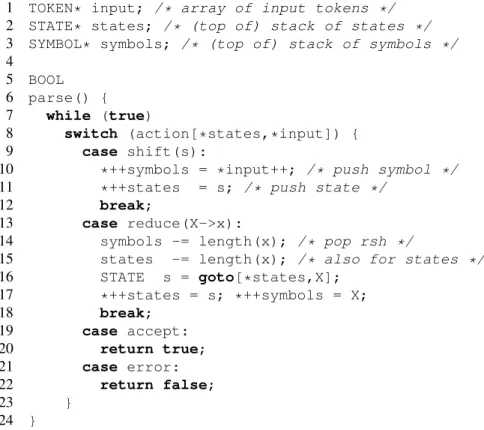
1 TOKEN* input; /* array of input tokens */
2 STATE* states; /* (top of) stack of states */
3 SYMBOL* symbols; /* (top of) stack of symbols */
4
5 BOOL 6 parse() { 7 while (true)
8 switch (action[*states,*input]) {
9 case shift(s):
10 *++symbols = *input++; /* push symbol */
11 *++states = s; /* push state */
12 break;
13 case reduce(X->x):
14 symbols -= length(x); /* pop rsh */
15 states -= length(x); /* also for states */
16 STATE s = goto[*states,X];
17 *++states = s; *++symbols = X;
18 break;
19 case accept:
20 return true;
21 case error:
22 return false;
23 } 24 }
Figure 3.9: Shift-reduce parser algorithm
Note that all states inNGare final. This does not mean thatNGaccepts any string
since there may be no transitions possible on certain inputs from certain states.
Intuitively, an item[A → α•β, a]can be regarded as describing the state where the parser hasαon the top of the stack and next expects to process the result of a derivation fromβ, followed by an input symbola.
To see that L(NG) accepts all viable prefixes. Consider a (partial)3 rightmost
derivation
S =X0 R
=⇒G x0X1y0 R
=⇒∗Gx0x1X2y1 R
=⇒∗G x0. . . xn−1Xnyn R
=⇒G x0. . . xn−1xnyn
whereyi ∈ Σ∗ for all0 ≤i ≤n, as depicted in Figure 3.10 where we show only
the steps involving the ancestors of the left hand side (Xn) of the last step (note
that none of thexi changes after being produced because we consider a rightmost
derivation).


![Figure 3.6: Predictive parser operation Algorithm 3 [Construction of LL(1) parse table]](https://thumb-us.123doks.com/thumbv2/123dok_us/8184871.2169792/47.892.123.715.190.911/figure-predictive-parser-operation-algorithm-construction-parse-table.webp)
![Figure 3.8: A shift-reduce parser Algorithm 6 [Shift-reduce parsing]](https://thumb-us.123doks.com/thumbv2/123dok_us/8184871.2169792/55.892.180.715.197.554/figure-shift-reduce-parser-algorithm-shift-reduce-parsing.webp)