ON THE SURFACE WIND STRESS FOR STORM SURGE MODELING
Jie Gao
A dissertation submitted to the faculty at the University of North Carolina at Chapel Hill in partial fulfillment of the requirements for the degree of Doctor of Philosophy in the Department
of Marine Sciences
Chapel Hill 2018
Approved by:
©2018 Jie Gao
ABSTRACT
Jie Gao: On The Surface Wind Stress For Storm Surge Modeling (Under the direction of Rick Luettich)
When wind blows over the open water, it exerts a shear stress at the water surface that transfers horizontal momentum vertically downward across the air–sea interface, driving the upper-ocean circulation, non-tidal sea surface elevation fluctuation, and formation of the surface wind waves. Thus, an accurate estimate of the surface wind stress is crucial to atmospheric, storm surge, and wave modeling. In this study, we have two major objectives: 1) development of a Generalized Asymmetric Holland Model (GAHM), and 2) implementation and evaluation of different surface drag laws for storm surge modeling.
Two major improvements over the classic Holland Model (HM) were made in this study. First of all, the assumption of cyclostrophic balance at radius to the maximum wind (RMW) was removed to eliminate the influence of the Rossby number (𝑅𝑜) on the gradient wind solution. Secondly, a composite wind method was employed to synthesize storm information from
multiple storm isotachs. The GAHM has been fully implemented in the ADCIRC model for real-time storm surge forecast, and initial model evaluation indicated an improved forecasting skill over the classic HM, especially when dealing with TCs with a small 𝑅𝑜.
It is generally accepted by the storm surge modeling community that the surface drag coefficient Cd increases linearly with wind speed at low to moderate winds and levels off or even
two explicit momentum flux models (RHG and DCCM), were implemented to study their behaviors under various wind and wave regimes, and to address the uncertainties in storm surge modeling. Initial evaluation suggested that the wave saturation tail level plays a big role in determining the surface stress, and the influence of the resolved part of the spectrum can be relatively small.Also, surge patterns were found to be greatly influenced by the spatial patterns of 𝐶𝑑, indicating a large uncertainty in storm surge modeling when using different drag laws. In the future, surge data of real hurricane cases are needed to quantify the performance of each drag law.
To my parents, and my dear husband Ao,
ACKNOWLEDGEMENTS
The success of this work was only possible with the contributions of my committee members, colleagues, and collaborators. First, I want to thank my advisor Rick Luettich for giving me the opportunity to work on this exciting topic in his lab. Being a great mentor, he provided plenty of guidance but also taught me to become an independent researcher. I also want to thank my committee members, Brian Blanton, Casey Dietrich, Johanna Rosman, and John Bane for giving me constructive ideas on my research topics, and providing guidance at different stages of my graduate studies. Also, many thanks to Tetsu Hara and Isaac Ginis at the University of Rhode Island for collaborating with us, and Brandon Reichl for providing source codes and documentation of RHG and DCCM. Chapter 3 was inspired by their previous works.
I thank members in our lab, including Jason Fleming, Crystal Fulcher, Tony Whipple, Ryan Neve, Jana Haddad, and Taylor Asher, for being there for me when I needed help. I also want to thank our IT support analyst Kar Howe and our student services manager Violet Anderson for their countless help.
TABLE OF CONTENTS
LIST OF TABLES ··· x
LIST OF FIGURES ··· xi
1. INTRODUCTION ··· 1
1.1 Parametric Vortex Wind Model ··· 1
1.2 Surface Wind Stress and Drag Coefficient ··· 3
1.3 Reviews of Commonly Used Surface Drag Laws ··· 4
GARRATT and GFDL14: Wind Speed-Dependent 𝐶𝑑 ··· 5
POWELL: Storm Sector-Dependent 𝐶𝑑 ··· 6
SWELL: DSPR-Dependent 𝐶𝑑 ··· 8
Wave Age and Wave Steepness: Wave Age- and Steepness-Dependent 𝑧0 ··· 10
1.4 Explicit Surface Wind Stress ··· 12
2. DEVELOPMENT AND EVALUATION OF A GENERALIZED ASYMMETRIC HOLLAND VORTEX MODEL ··· 16
2.1 Introduction ··· 16
2.2 Model Description ··· 21
2.2.1 The classic Holland Model (1980) ··· 21
2.2.2 Derivation of GAHM’s Formulas ··· 23
2.2.3 Calculation of the Spatially Varying RMW ··· 27
2.3 Study Cases ··· 32
2.4 Model Results using the Single-Isotach Approach ··· 38
2.4.1 Model Consistency at Distances to the Highest Isotach ··· 38
2.4.2 Evaluation of the RMW and the Modeled Maximum Wind ··· 40
2.5 Model Results using the Multiple-Isotach Approach ··· 42
2.5.1 Evaluations of Composite Wind Fields ··· 43
2.5.2 Model Consistency at Distances to All Available Isotach ··· 47
2.6 Summary and Discussion ··· 49
3. EXPLICIT SURFACE WIND STRESS UNDER TROPICAL CYCLONES FOR STORM SURGE MODELING ··· 52
3.1 Introduction ··· 52
3.1.1 RHG and DCCM ··· 52
3.1.2 Objectives ··· 55
Sensitivity Study of the Explicit Surface Wind Stress on diagnostic tail and prognostic 2D spectrum ··· 56
Impact of Different Drag Laws on Storm Surge Modeling ··· 57
3.2 Methodology ··· 58
3.2.1 Implementation of Sea State Dependent Stress in the Coupled ADCIRC + SWAN ··· 58
3.2.2 Experimental Design ··· 61
Experiment A ··· 62
Experiment B ··· 62
3.3 Sensitivity Study of the Explicit Sea State Dependent Stress ··· 62
3.3.3 Sensitivity of 𝐶𝑑 to Prognostic Wave Spectrum
and Diagnostic spectral tail ··· 77
Deep Water ··· 77
Shallow Water ··· 81
3.3.4 Summary and Conclusions ··· 85
3.4. Storm Surge Study using Different Drag Laws ··· 86
3.4.1 Drag Comparison among Different Methods ··· 86
3.4.2 Influence on Storm Surge ··· 90
3.4.3 Summary and Conclusions ··· 92
4. DISCUSSION AND CONCLUSIONS ··· 94
4.1 Discussion on the GAHM ··· 94
4.2 Discussion on Surface Wind Stress and Storm Surge Modeling ··· 95
LIST OF TABLES
Table
2.1 Meteorological details of seven recent hurricanes listed
in chronological order ··· 33
2.2. Parameters of storm characteristics at three snapshots of Irene (2011) ··· 38
2.3. Statistical analysis of modeled winds at distances to all isotachs based on all seven storms ··· 49
3.1. Drag laws in ADCIRC ··· 56
3.2. Physics packages in SWAN ··· 58
3.3 Input and output list for RHG and DCCM ··· 59
LIST OF FIGURES
Figure
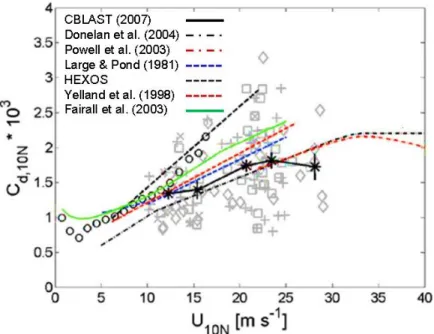
1.1 Measured 𝐶𝑑 from different field and laboratory studies, showing a large spread (Black et al. (2007)). The squares, plus signs, and diamonds are CBLAST observations from different quadrants of
the storms. ··· 4 1.2 Comparison of 𝐶𝑑 among GARRATT (capped at 2.5 × 10⁻³),
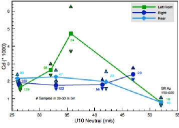
GFDL14, and SWAN-FIT. ··· 6 1.3 Different behaviors of 𝐶𝑑 in the rear, right and left storm sectors
by Powell et al. (2007)··· 7 1.4 𝐶𝑑 values sorted over three storm sectors by Holthuijsen et al. (2012). ··· 9 1.5 The geographic pattern of the calculated wave directional spreading
for Hurricane Luis (1995) in Panel A and Fran (1996) in Panel B by Holthuijsen et al. (2012). The contours of 𝜎𝜃 = 45° and 𝜎𝜃 = 50° are indicated with black dashed lines. Black arrow indicates the
hurricane motion. ··· 9 1.6 (A) The drag coefficient of Ho12 via (1.8), and (B) The drag
coefficient with the expression of Wu (1982) capped at 2.5 × 10⁻³ by
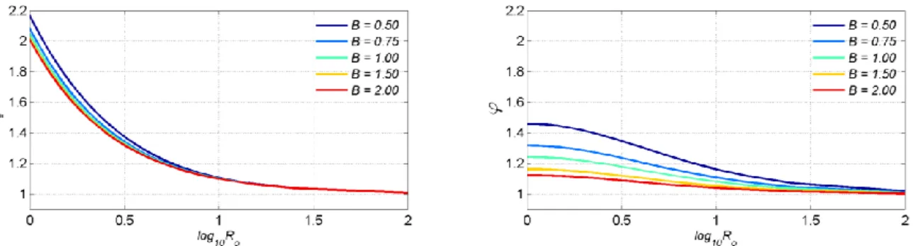
Holthuijsen et al. (2012). ··· 10 2.1 Profiles of 𝐵𝑔⁄𝐵 (left panel) and 𝜑 (right panel) with respect
to log10𝑅𝑜, given different 𝐵 values as shown in different colors. ··· 25 2.2 The normalized gradient wind profiles of the HM (left panel)
and the GAHM (right panel) as functions of the normalized radial
distances and 𝑅𝑜, given different Holland 𝐵 values. ··· 26 2.3 Slices of the normalized gradient wind profiles (as shown in Figure 2.2)
at log10𝑅𝑜 = 0, 1, 𝑎𝑛𝑑 2 (or correspondingly 𝑅𝑜 = 1, 10, 𝑎𝑛𝑑 100). ··· 27
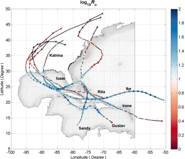
2.4 Best tracks and Intensity of seven selected Hurricanes used in this study. Black lines represent hurricane best tracks, and dots represent data entries with 6-hour intervals (occasionally there
are exceptions), colored by the maximum sustained wind. ··· 35 2.5 Same as Figure 2.4, but dots are colored by Holland 𝐵. ··· 36 2.6 Same as Figure 2.4 but dots are colored by 𝑅𝑜 in base 10
2.7 Radial wind profiles of Irene (2011) at three different stages. Vertical bars represent the storm isotachs reported in NHC’s “best track” file. The highest isotach (utilized) in each quadrant
are plotted in black, while lower isotachs (not utilized) are in gray. ··· 39 2.8 Comparison of the modeled and “Best Track” 𝑉𝑚 (upper two panels)
and the modeled and “Best Track” 𝑅𝑚𝑎𝑥 (lower two panels)
between the AHM and the GAHM based on all seven hurricanes. ··· 41 2.9 Three-dimensional snapshots of Irene’s radial wind profiles (left)
and interpolated spatial wind field (right) by the single-isotach approach (upper two panels) and the multiple-isotach approach
(lower two panels). ··· 43 2.10 Three snapshots (in columns) of Irene’s two-dimensional wind
fields by the AHM, GAHM, SLOSH, H*Wind and OWI winds
corresponding to Table 2.2. ··· 45 2.11 Comparison of the modeled and “Best Track” 𝑉𝑚 (upper five panels)
and the modeled and “Best Track” 𝑅𝑚𝑎𝑥 (lower five panels) based on all seven hurricanes between the AHM, the GAHM, the SLOSH,
|the H*Wind and OWI winds. ··· 46 2.12 GAHM’s composite radial wind profiles of Irene (2011) at 3
different developing stages. Vertical bars represent all available
storm isotachs reported in NHC’s “best track” file. ··· 48 2.13 Comparison of specified isotachs and modeled winds at distances
to specified isotachs for all seven selected hurricanes. ··· 49 3.1 Directionally integrated saturation spectrum simulated in WWIII
with WWIII original tail, three constant tail level options, and empirical tail of Elfouhaily et al., 1997 for (a) 10 m/s wind, and (b) 40 m/s wind experiments. Three vertical dashed lines represent wavenumbers corresponding to 𝑓𝑝, 1.25 × 𝑓𝑝, and 3 × 𝑓𝑝
(Reichl et al., 2014). ··· 54 3.2 Coupling different drag laws to ADCIRC+SWAN. ··· 59 3.3 Intensity and Best Track of Hurricane Irene (08/20/2011 00:00:00
– 08/29/2011 00:00:00 UTC). Model results are investigated at
two instances indicated by the circles. ··· 61 3.4 Spatial wind field at two snapshots: 08/26/2011 03:00 UTC
(left panel) and 08/28/2011 21:00 UTC (right panel). Diagnostic
3.5 Comparison of 1-D wave spectra (left column) and the corresponding saturation spectra (right column) among Komen, Janssen, and Westhuysen in SWAN at eight stations (shown with different colored lines) at the first snapshot
(08/26/2011 03:00 UTC). Three vertical (dashed) lines from left to right in each panel represent the wavenumbers corresponding
to 𝑓𝑝, 1.2 × 𝑓𝑝, and 3 × 𝑓𝑝 of the first station. ··· 65
3.6 Comparison of 1-D wave spectra (left column) and the corresponding saturation spectra (right column) attached with the Reichl’s empirical tail among three different physics packages at the first snapshot. ··· 66
3.7 Comparison of 1-D wave spectra (left column) and the corresponding saturation spectra (right column) attached with the extended tail among three different physics packages at the first snapshot. ··· 67
3.8 Same as Figure 3.5 but at the second snapshot (08/28/2011 21:00 UTC). ··· 68
3.9 Same as Figure 3.6 but at the second snapshot (08/28/2011 21:00 UTC). ··· 69
3.10 Same as Figure 3.7 but at the second snapshot (08/28/2011 21:00 UTC). ··· 70
3.11 Wave spectra, saturation spectra, and integrated wave form stress profiles at 08/26/2011 03:00 UTC: a) Directionally integrated SWAN wave spectra using Komen physics package, b) SWAN saturation spectra, c) SWAN spectra with Reichl’s empirical tail, d) Saturation spectra with Reichl’s empirical tail, d) 1-D wave form stress over k, e) CDF of 1-D form stress over k. ··· 73
3.12 Wave spectra, saturation spectra, and integrated wave form stress profiles at 08/26/2011 03:00 UTC for the extended tail option at 08/26/2011 03:00 UTC. ··· 74
3.13 Same as Figure 3.11, except at 08/28/2011 21:00 UTC when wave field reaches steady state. ··· 75
3.14 Same as Figure 3.12, except at 08/28/2011 21:00 UTC when wave field reaches steady state. ··· 76
3.15 Spatial plot of wind speed, 𝐶𝑑, Saturation tail level, and DSPR at 08/26/2011 00:00 UTC for Reichl’s empirical tail option. ··· 79
3.17 3D plot of Wind (x), DSPR (y), 𝐶𝑑 (z) and Saturation level B (color) for Reichl’s empirical tail option (upper panel)) and the extended
tail (lower panel)) at 08/26/2011 00:00 UTC. ··· 81
3.18 Same as Figure 3.15 for Reichl’s empirical tail option, but for shallow water at 08/26/2011 00:00 UTC. ··· 83
3.19 Same as Figure 3.16 for the extended tail option, but for shallow water at 08/26/2011 00:00 UTC. ··· 84
3.20 Same as Figure 3.17, but for shallow water at 08/27/2011 06:00 UTC. ··· 85
3.21 Spatial plots of the wind speed, 𝐶𝑑 from DCCM, water elevation and a few wave for the deep water condition at 08/26/2011 00:00:00 UTC. ··· 87
3.22 Spatial distribution of 𝐶𝑑 among different drag laws at 08/26/2011 00:00:00 UTC. Upper panels from left to right: Garratt, GFDL14, Powell, Swell (Ho12). Lower panels from left to right: RHG, DCCM, Wave Age (D03) and Wave Steepness (YT01). ··· 88
3.23 Comparison of 𝐶𝑑 as a function of wind speed at 08/26/2011 00:00:00 UTC. ··· 88
3.24 Same as Figure 3.21, but at 08/27/2011 06:00:00 UTC. ··· 89
3.25 Same as Figure 3.22, but at 08/27/2011 06:00:00 UTC. ··· 90
3.26 Same as Figure 3.23, but at 08/27/2011 06:00:00 UTC. ··· 90
3.27 Spatial plot of Maximum water elevation resulted from different drag laws. ··· 91
CHAPTER 1: INTRODUCTION
1.1 Parametric Vortex Wind Model
Timely and accurate estimate of the surface pressure and wind fields of a tropical cyclone (TC) is critical to storm surge forecasting and coastal risk assessment. Currently, prediction of a TC’s wind field can be achieved through multiple approaches. One approach is through the use of atmospheric models, which are either statistical, dynamical, or combined
statistical-dynamical, to obtain wind forecasts or nowcasts. The statistical ones empirically predict the evolution of a TC by extrapolating from historical datasets, while the dynamical models solve the full set of primitive equations of fluid flow in the atmosphere to obtain numerical results, which are quite computationally intensive.
In recent years, the kinematic analysis approach showed promise to offer more realistic and accurate wind estimates, either in real-time or in hindcast mode. One example is the Surface Wind Analysis System (H*Wind) operated by the Hurricane Research Division (HRD) before 2014, which produces H*Wind snapshots of TCs from 1993 – 2013 by assimilating all available surface wind observations (e.g., from ships, buoys, coastal platforms, reconnaissance aircrafts, and satellites, etc.) into a common framework for height (10m), exposure, and averaging period (Powell et al., 1996). Given its versatile inputs, the H*Wind products are considered to be among the most sophisticated and reliable surface wind reconstructions.
field of a TC can be estimated as the sum of the storm vortex winds and the background winds of the environment. The vortex winds are usually depicted by a radial wind profile, whose formula is either derived from the gradient or cyclostrophic wind balance equation, or simply an
empirical expression acquired from historical storm events. The background winds are of a much larger scale, and among other factors, are responsible for steering the movement of a TC
(Shapiro, 1983) and considered to account for some of the asymmetry observed in the overall wind field. Currently, there is no clear consensus on how to determine the distribution of
background winds due to insufficient observational data. In many applications, it was common to set the background winds equal to the storm’s translational velocity 𝑉⃗⃗⃗⃗ 𝑇 (e.g., Powell et al., 2005; Mattocks and Forbes, 2008), while in many others, the background winds were assumed to be in the same direction as 𝑉⃗⃗⃗⃗ 𝑇 but with reduced magnitudes by various factors (e.g., radially varies between 0-0.5 by Jelesnianski et al., 1992, Phadke et al., 2003, and Hu et al., 2012; azimuthally varies between 0-0.5 by Georgiou, 1985, and Xie et al., 2006; constant 0.6 by Emanuel et al., 2006; constant 0.5 by Lin et al., 2012a). Lin and Chavas (2012b) introduced a methodology via vector decomposition of H*Wind surface wind fields to investigate the relationship between the surface background winds and 𝑉⃗⃗⃗⃗ 𝑇, and found that statistically the surface background winds are reduced by a factor of 𝛼 = 0.55 and rotated counter-clockwise (in the Northern Hemisphere) by an angle of 𝛽 =20° relative to 𝑉⃗⃗⃗⃗ 𝑇.
1.2 Surface Wind Stress and Drag Coefficient
When wind blows over the open water, it exerts a shear stress at the water surface that transfers horizontal momentum vertically downward across the air–sea interface, driving the upper-ocean circulation, non-tidal sea surface elevation fluctuation, and formation of the surface wind waves. Thus, an accurate estimate of the surface wind stress is crucial to atmospheric, storm surge, and wave modeling. In common practice, the surface wind stress in storm surge model is parameterized using the bulk formula
𝜏⃑ =𝜌𝑎𝐶𝑑𝑈⃗⃗⃑10|𝑈⃗⃗⃑10| , (1.1)
where 𝜌𝑎is the density of air, 𝐶𝑑 is the surface drag coefficient, and 𝑈⃗⃗⃑10is the wind speed at 10m height. Assuming neutral stability, the mathematical representation of the mean wind velocity profile within the atmospheric boundary layer (ABL) is given by the logarithmic law
𝑢𝑢
∗
=
1 𝜅𝑙𝑛𝑧
𝑧0, (1.2)
where 𝑢 is the wind speed at height 𝑧, 𝜅 is the von Karman constant (determined experimentally to be ~0.40), 𝑧0is the surface roughness length, and 𝑢∗ is the friction velocity defined by
|𝜏 | = 𝜌𝑎𝑢∗2 . (1.3)
Charnock (1955) proposed that a simple non-dimensional relation exists between 𝑧0 and 𝑢∗
𝛼 =𝑧0𝑔
𝑢∗2 , (1.4)
condition of the ocean surface with respect to wave characteristics such as wave height, period, or wave spectrum at a given time and location. Based on Eqs. 1.1~1.4, 𝐶𝑑can be rewritten as
𝐶𝑑= (|𝑈⃗⃗⃑𝑢∗ 10|)
2
or 𝐶𝑑 = (𝜅 𝑙𝑛 (10𝑧 0)
⁄ )2. (1.5)
The drag coefficient therefore can be regarded as a measure of the roughness of the sea, and is influenced by many factors such as the wind speed, atmospheric stability, and sea state, etc.
1.3 Reviews of Commonly Used Surface Drag Laws
Many approaches have been developed to estimate the surface wind stress 𝜏⃑ (or described in terms of surface roughness 𝑧0 or surface drag coefficient 𝐶𝑑). However, results are far from conclusive, especially under a wide range of wind and wave regimes (Figure 1.1). In this section, a few common surface drag laws are described in detail.
GARRATT and GFDL14: Wind Speed-Dependent 𝑪𝒅
The majority of previous studies were conducted in low to moderate wind regimes lower than 25 m/s. Their results suggest that 𝐶𝑑is wind speed-dependent and can be expressed as a linear function of |𝑈⃗⃗⃑10|(e.g., Garratt, 1977; Smith, 1980; Large and Pond, 1981; Wu, 1982; Yelland and Taylor, 1996)
𝐶𝑑× 103= 𝑎 + 𝑏|𝑈⃗⃗⃑10|, (1.6)
where parameters 𝑎 and 𝑏 are empirically determined. For the GARRATT drag law, a= 0.75 and b=0.067. Equation (1.6) predicts a monotonic increase of 𝐶𝑑 with wind speed, and in extreme wind speeds values of 𝐶𝑑are simply extrapolated. Wind measurements under hurricane wind forcing were made available via the use of the Global Positioning System (GPS) dropsondes. Powell et al. (2003, hereinafter P03) analyzed 331 GPS dropsonde data from 15 storms (1997-1999) and concluded that, contrary to previous thoughts, 𝐶𝑑 tends to level off around ~34 m/s and then decrease with increasing wind speed, possibly due to air-flow separation and the existence of sea spay and white-capping at high winds. Laboratory tank measurements by Donelan et al. (2004) and theoretical studies by Soloviev et al. (2014) predicted a similar behavior of 𝐶𝑑 to drop off at high wind speeds. To adopt these new findings, a cap value can be simply applied to existing formulas to represent the leveling off of 𝐶𝑑 at high wind speeds. In ADCIRC, Garratt’s formula is typically capped at 2.5 × 10⁻³ or 3.5 × 10⁻³.
A more sophisticated approach is to fit a polynomial curve to capture the leveling off and then decreasing of 𝐶𝑑 at high wind speeds, such as the GFDL14 drag law used in the GFDL hurricane model, and SWAN-FIT, the 2nd order polynomial implemented in SWAN (Zijlema et
Figure 1.2. Comparison of Cd among GARRATT (capped at 2.5 × 10⁻³), GFDL14, and SWAN-FIT.
POWELL: Storm Sector-Dependent 𝑪𝒅
In the Coupled Boundary Layer Air-Sea Transfer (CBLAST, 2000-2005) field experiment, Black et al. (2007) identified three storm sectors with distinctive wave
characteristics, partitioned by the 20°, 150° and 240° angle relative to the storm forward motion: 1) Rear sector with unimodal, short-wavelength (~150 - 200m) waves moving with the wind, 2) Right sector with bimodal or trimodal spectra shifting to longer wavelengths (~200 - 300m) moving outward by up to 45° relative to the wind directions, and 3) Left sector with unimodal spectra, peak long-wavelength waves (~200 - 350m) moving outward relative to the wind by 60° - 90°.
constant and decreases at wind speed above 34 m/s, 2) In the right sector (20 - 150°), 𝐶𝑑is relatively constant with wind speed, but a slight increase was suggested at wind speed above 45 m/s, and 3) In the front left sector (241 – 20°), 𝐶𝑑is the most sensitive to wind speed, and increases to a maximum value of 4.7 × 10⁻³at wind speed of 36 m/s and then decreases rapidly at higher winds.
Powell’s findings contradicted numerical modeling results by Moon et al. (2004), who estimated a higher 𝐶𝑑 in the right and front of the storm where longer, higher, and more fully developed waves dominate, and a lower 𝐶𝑑 in the rear and left of the storm with shorter and younger waves. It is recommended that further investigations be conducted in light of this inconsistency. Powell’s storm sector-dependent 𝐶𝑑 formula has been implemented in ADCIRC (Dietrich, 2010) as an alternative to Garratt’s formula.
SWELL: DSPR-Dependent 𝑪𝒅
Partition of the three storm sectors in Black et al. (2007) is always conducted at fixed angles relative to the storm forward motion, and the attribution of swell type is always categorized (following, opposing or cross swell). Parameterization of 𝐶𝑑 based on three swell types is problematic, as the physical processes influencing the surface wind drag should not vary discontinuously with swell type and in geographic space, and should not depend on storm
forward motion. To resolve this issue, Ho12 proposed to grade swell type continuously using the wave directional spreading variable DSPR 𝜎𝜃, which by definition accounts for the swell in proportion to its energy relative to the energy of local windsea. DSPR is defined as (in analogy with the definition of standard deviation):
𝜎𝜃2 = 〈𝑠𝑖𝑛2(𝜃)〉, (1.7)
where 𝜃 is the wave direction elative to the mean wave direction, and the operator 〈 〉represents the average over spectral direction weighted with wave energy density (Battjes, 1972). Typically,
𝜎𝜃 is ~30° for a pure windsea without swell (Holthuijsen, 2007), and grows significantly larger if crossing and opposing swell exist.
Ho12 sorted the 𝐶𝑑 values obtained from 1149 GPS dropsondes wind profiles (1998-2005) over the three storm sectors (or equivalently the three types of swell) in different wind speed groups (Figure 1.4), and derived an informally fitted empirical expression of 𝐶𝑑 in terms of
|𝑈⃗⃗⃑10|as a preliminary assessment:
𝐶𝑑× 103= 𝑚𝑖𝑛 {[𝑎 + 𝑏 (|𝑈⃗⃗⃑10| |⁄𝑈⃗⃗⃑𝑟𝑒𝑓,1|) 𝑐
] , 𝑑 [1 − (|𝑈⃗⃗⃑10| |⁄𝑈⃗⃗⃑𝑟𝑒𝑓,2|) 𝑒
Figure 1.4. 𝐶𝑑 values sorted over three storm sectors by Holthuijsen et al. (2012)
Based on case studies of Hurricane Luis (1995) and Fran (1996), Ho12 found that the 45° and 55° contour lines of 𝜎𝜃 corresponded reasonably well with the boundaries of the three storm sectors (Figure 1.5), which provides the range of validity of (1.8) and its coefficients in terms of
𝜎𝜃.
Figure 1.5. The geographic pattern of the calculated wave directional spreading for Hurricane Luis (1995) in Panel A and Fran (1996) in Panel B by Holthuijsen et al. (2012). The contours of 𝜎𝜃= 45° and
𝜎𝜃 = 50° are indicated with black dashed lines. Black arrow indicates the hurricane motion.
parameterization obviously would result in different outcomes in wind, wave, and storm surge predictions if it were used. We plan to implement and test the Ho12 parameterization in the coupled ADCIRC and SWAN model in the future.
Figure 1.6. (A) The drag coefficient of Ho12 via (1.8), and (B) The drag coefficient with the expression of Wu (1982) capped at 2.5 × 10⁻³ by Holthuijsen et al. (2012).
Wave Age and Wave Steepness: Wave Age- and Steepness-Dependent 𝒛𝟎
It has long been recognized that sea state plays an important role in affecting the surface momentum flux at the air-sea interface, and many attempts have been made to relate surface wind stress (or equivalently 𝐶𝑑, 𝑧0 or 𝛼) to wave parameters that characterize the sea state. Consider a pure windsea with a single spectral peak, free of contamination from swell. The windsea usually has a universal spectral shape that results from the coupled system of wind, wind waves, and surface currents. Therefore, the local windsea can be characterized by the phase velocity at the spectral peak 𝑐𝑝, and similarly, the momentum flux through the coupled system can be characterized by 𝑢∗or|𝑈⃗⃗⃑10|. Thus, it is possible to represent the developmental stage of the sea with a dimensionless “wave age” 𝑐𝑝⁄𝑢
Thus, wave age is a plausible candidate to describe the sea surface roughness. Kitaigorodskii and Volkov (1965) made the first attempt to relate sea surface roughness to the sea state, and
proposed that the Charnock’s constant 𝛼 depends on wave age. Since that, numerous efforts have been made in the field and laboratories to find the relation between 𝑧0 and 𝑐𝑝⁄𝑢∗, but no
definitive conclusions have been reached (e.g., Geernaert 1986; Toba et al. 1990; Smith et al. 1992; Donelan et al. 1993; Oost et al. 2002; Drennan et al. 2003). Part of the problem lies in the fact that by definition both 𝑧0 and wave age depend on 𝑢∗, which could lead to potential spurious correlations between these two variables (Kenney, 1982). To eliminate the issue, Drennan et al. (2003, hereinafter D03) combined five datasets of different sources that represent a variety of wind-wave conditions, and concluded that a power-law relation exist between 𝑧0⁄𝐻𝑠 and the inverse wave age
𝑧0⁄𝐻𝑠 = 3.35(𝑢∗⁄ )𝑐𝑝 3.4 , (1.9)
where 𝐻𝑠 is the significant wave height. Equation (1.9) implies that younger waves are rougher than older waves. Note that for wind-waves in local equilibrium with the wind, there is a strong statistical interdependence between the variables in (1.9) Thus, the extent to which the wave age-dependent formula differs from or has in common with the conventional wind speed-age-dependent formula under different wind-wave conditions is a question that needs to be answered. Also, a clear wave age-dependent surface drag has not been observed in open ocean under hurricane wind forcing, so we should be cautious to use it in storm surge modeling.
Hsu (1974) took a different path to relate surface roughness to the sea state, and suggested that 𝑧0 depended on the wave slope 𝐻𝑠⁄𝐿𝑝, where 𝐿𝑝 is the wavelength of waves at
(2001, hereinafter TY01) proposed a wave steepness-dependent formula, which predicts a power law relation between the dimensionless roughness 𝑧0⁄𝐻𝑠 and steepness of the dominant waves
𝑧0⁄𝐻𝑠 = 1200(𝐻𝑠⁄ )𝐿𝑝 4.5 . (1.10)
Using this formula, the roughness changes due to fetch or duration limitations are small. Equation (1.10) reconciles many observations that previously had appeared scattered, except for data corresponding to very young waves. Drennan et al. (2005) evaluated both D03 and TY01 using eight assembled datasets, and found that these two methods yielded rather different estimates of roughness depending on the sea states. Each method has its own merits and
limitations: 1) in conditions with a dominant wind sea, both methods yield better estimates than the traditional bulk formula, 2) in general conditions with mixed sea, the steepness method performs better, 3) for underdeveloped younger wind sea, the wave age method yields better results, and 4) for swell-dominated conditions, neither methods did well. Implementation of both methods does not require explicit knowledge of the wave spectrum.
1.4 Explicit Surface Wind Stress
Wave field associated with a hurricane is rather complex both in space and time due to the translational nature of a hurricane and the curvature of the winds, an explicit
parameterization of surface wind stress that depends on the 2D wave spectrum is desired. We hope that by incorporating the 2D wave spectrum (both the long wave spectrum and short wave spectrum tail) into the stress formulations, more physics can be captured to explain the large amount of scatters in the surface drag measurements.
waves. The most important contribution on the shape of wave spectrum comes from the JOint North Sea WAve Project (JONSWAP, Hasselmann et al., 1973), in which a universal spectral shape (normalized over spectral peak) was found for waves in idealized fetched-limited, deep water conditions. Waves in the equilibrium range are quasi-saturated, meaning that their slope is limited by breaking and does not increase much with wind speed. Up until now, our knowledge of the wave spectrum in the equilibrium range is still limited, especially under high wind conditions. There is debate over the shape of the high frequency spectral tail, but the 𝑓−5 tail (Phillips, 1958; Pierson and Moskowitz, 1964; JONSWAP, Hasselmann et al., 1973) and the 𝑓−4 tail (Toba, 1973; Donelan et al., 1985; Hwang et al., 2000) are most widely used. Note, wave spectra in wavenumber space and in frequency space can be inter-changed using straightforward Jacobian transformations. The 𝑘−4 tail corresponding to the 𝑓−5 tail in frequency spectrum is most often used in a wavenumber spectrum. Numerical wave models typically resolve wave spectrum to a certain frequency, and an empirical tail needs to be attached to extend the spectrum to high frequency range.
Based on conservation of momentum in the marine boundary layer, Janssen (1989) and later Chalikov and Makin (1991) introduced a theory that takes into account the directional wavenumber spectrum Ψ(𝑘, 𝜃) to describe the exchange of momentum at the air-sea interface, where Ψ(𝑘, 𝜃) is defined as
𝜂̅̅̅ = ∫ ∫ Ψ(𝑘, 𝜃)𝑑𝜃𝑘⃗⃑𝑑𝑘⃗⃑2 0𝑘 −𝜋𝜋 , (1.11)
with 𝜂̅̅̅2 being the mean square surface displacement. The total stress is supported by both the turbulent motions of the air 𝜏𝑡 and the wave-induced motions due to the wind waves 𝜏𝑓
At the sea surface 𝑧 = 0 the total flux equals to the sum of the viscous stress 𝜏𝜈 ≡ 𝜏𝑡(0) and form stress 𝜏𝑓≡ 𝜏𝑓(0). The viscous stress comes through the direct molecular interaction at the surface, and can be calculated from the law of smooth wall, with viscous drag coefficient adjusted for the sheltering effect in the presence of waves (Donelan et al., 2012), and the form stress is given by the rate of change of wave momentum in time due to the wind source input
𝜏⃑𝑓 = ∫𝜕𝑡𝜕 𝑃⃗⃑𝑤𝑖𝑛𝑑𝑑𝑘⃗⃑. (1.13)
To characterize the input rate of momentum from the atmosphere to waves, here we define
𝜕𝑡𝜕 𝑃⃗⃑𝑤𝑖𝑛𝑑 = 𝛽(𝑘, 𝜃)𝑃⃗⃑𝑤𝑖𝑛𝑑, (1.14)
where 𝑃⃗⃑𝑤𝑖𝑛𝑑 is the pressure exerted on the water surface by wind, and 𝛽(𝑘, 𝜃) is the wave
growth rate. Parameterization of 𝛽(𝑘, 𝜃) varies in different studies. Assuming dispersion relation
𝜔2 = 𝑔𝑘, the wave momentum is given by (Phillips, 1977)
𝑃⃗⃑𝑤𝑖𝑛𝑑 = 𝜌𝑤𝜔𝑘Ψ(𝑘, 𝜃)𝑘⃗⃑, (1.15)
where 𝜌𝑤 is the density of water, and 𝜔 is the wave frequency. Combining Eqs. (1.13~1.15), the form drag can be expressed as
𝜏⃑𝑓= 𝜌𝑤∫ ∫ 𝜔𝛽(𝑘, 𝜃)Ψ(𝑘, 𝜃)𝑑𝜃𝑘⃗⃑𝑑𝑘⃗⃑0𝑘 −𝜋𝜋 (1.16)
these types of model is that the form drag calculated using (1.16) is very sensitive to the high frequency tail, and there is little known about the spectral tail under hurricane wind conditions.
CHAPTER 2: DEVELOPMENT AND EVALUATION OF A GENERALIZED ASYMMETRIC HOLLAND VORTEX MODEL
2.1 Introduction
There are many kinds of parametric wind models exist, which use similar sets of storm parameters but distinct methods to offer TC pressure and wind estimates. One example is the SLOSH (Sea, Lake, and Overland Surges from Hurricanes, Jelesnianski et al., 1992) wind model, which is among the most important features of the SLOSH storm surge model currently used by the National Weather Service (NWS) for storm surge guidance. The SLOSH describes a circularly-symmetric storm vortex superimposed upon the background winds calculated from 𝑉⃗⃗⃗⃗ 𝑇. It takes the radius to maximum wind (RMW) and central pressure deficit as its key model inputs, and first estimates the maximum windempirically and then solves for the pressure and wind fields. Houston et al. (1999) did a model comparison between analyzed wind observations and the SLOSH modeled winds for seven cases in five hurricanes, and found that the SLOSH under-estimated the peak winds by 15% in Hurricane Emily (1993), and by 6% or less in the rest cases. Also, the mean wind speed and mean inflow angle for the SLOSH winds were 14% stronger and 19° less than those observed in the region of strongest winds.
the gradient wind equation, the RMW is found to be entirely defined by A and B, independent of the central pressure deficit and the maximum wind. It is logical to speculate that the
cyclostrophic assumption is only reasonable when the Rossby number (𝑅𝑜, which is a
dimensionless number relating the ratio of nonlinear accelerations to the Coriolis force) at the RMW is large (details given in section 2.2.2). A great feature of the HM is that both A and B, as well as the RMW if it is absent from model inputs, can be readily derived from a limited set of wind observations, or determined climtologically for a standard hurricane. This feature is extremely useful when the RMW is not available at the time of forecasting. For example, in the event of a TC, the National Hurricane Center (NHC) issues forecast advisories every six hours to update the current and future (forecasts made for 12, 24, 36, and 72 hours from the current synoptic time) storm location, the central pressure, the observed maximum sustained wind, the radii to the specified 34-, 50-, and 64-kt storm isotachs in each of the NorthEast (NE), SoutEast (SE), SouthWest (SW), and NorthWest (NW) storm quadrants, etc. Based on the radius to a specified isotach in one quadrant, the RMW can be solved by fitting the isotach data to the HM’s wind profile via a root-finding algorithm. The HM uses an azimuthally constant RMW to
construct its axis-symmetrical wind field. Given their simplicity and reasonable forecasting skill, the HM and its variants have been used extensively for operational forecasting of TC winds over the past few decades.
these issues, Willoughby et al. (2006, WM) proposed a new family of sectionally continuous profiles that allow the wind to increase in proportion to a power of radius inside the eye and decay exponentially outside the eye with a smooth transition in between. Unlike the HM, which is a pressure-wind relationship model, the WM calculates the geopotential height of a given pressure through an outward integration of the gradient wind acceleration. The storm parameters featured in the WM, including the exponent for the power law inside the eye, and a single- (dual-) exponential decay length(s) outside the eye, were derived using lease square fits based on a sample of 493 observed profiles, and accurate estimation of these parameters require ample wind data both inside and outside the storm eye. The WM’s wind profile was shown to fit historical wind observations more accurately. However, in the event of a TC when only limited storm information is available at the time of forecasting, statistically fitted parameters from historical TC events might not lead to an optimum fit to each individual storm.
Another attempt was made by Wood et al. (2013, hereafter WW13) to extend the existing tangential wind model of Wood and White (2011) and tailor it for TC application. The WW13 proposed a partitioned TC wind profile that was able to render as many as three wind maxima during an Eye Replacement Cycle (ERC). It features five key storm parameters in each of its primary, secondary, and tertiary tangential wind formulations: the RMW, the maximum wind, and three shape parameters including the growth parameter 𝜅, and the decay parameter 𝜂, and the size parameter 𝜆. Each intuitive shape parameter has its unique physical meaning and acts
independently in controlling different portions of the wind profile. In the WW13, the gradient wind is readily derived from the cyclostrophic wind in terms of the cyclostrophic Rossby number
𝑅𝑜𝐶, and the total pressure profile is partitioned into different components corresponded with the multi-maxima wind profile, calculated via cyclostrophic balance. It was noted that the WW13 was optimized to define a relatively peaked TC with a large 𝑅𝑜𝐶 that typically ranging from 10 to 100 (Willoughby, 1990; Willoughby and Rahn, 2004). For a TC with a relatively broad profile and 𝑅𝑜𝐶 less than 10, the RMW was often found to be displaced towards the TC center, and both the RMW and the maximum wind needed to be mathematically adjusted. The WW13 showed sophistication in obtaining optimum fit to known radial profiles, but it also requires an accurate estimate of the RMW as input data to accomplish that, which may render it inconvenient for operational forecasting.
Naturally, there is considerable variability in the estimated surface wind fields
RMW as input data allow the HM to be widely used for operational forecasting. Based on the HM, Xie et al. (2006) developed a real-time hurricane surface wind forecasting system that is characterized by an azimuthally-varying RMW for better depicting surface wind structure of an asymmetric TC such as a land falling hurricane, a.k.a. the asymmetric Holland model (AHM). Using radii to the highest isotach (34, 50, or 64 kt) in each of the 4 storm quadrants, the RMW is calculated in each quadrant and then fitted azimuthally around the storm center via a polynomial interpolation.
Mattocks et al. (2006) implemented Xie’s work in the ADCIRC model (Luettich,
Westerink, and Scheffner, 1991; Westerink et al., 1992) and uses the coupled model for real-time storm surge and wave forecasting for the state of North Carolina. This operational system has many advantages: 1) it allows an ocean simulation to be launched as soon as an NHC forecast advisory is issued, usually hours before other numerical wind products become available, 2) a synthetic wind field is computed on the fly at each time step during the entire simulation period, and 3) by varying storm parameters, such as storm track or storm forwarding speed, a series of ensemble members of forecasts for strategic assessment of coastal emergencies can be provided. As an improved application of the HM, the AHM works great for intense but relatively narrow TCs with a large 𝑅𝑜, for which the cyclostrophic assumption made at the RMW is valid. However, for a generally weak but broad TC, or a strong TC at its developing or dissipating stages, the AHM is inferior as the Coriolis force is no longer negligible at the RMW. Cases like these will mostly lead to underestimations of the peak winds, as well as unrealistic wind profiles in the AHM.
that by eliminating the cyclostrophic assumption at the RMW, the GAHM should be able to generate high-quality representative wind fields for a wide range of TCs. Also, a composite wind method should be implemented in the GAHM in order to fully use all multiple storm isotachs in NHC’s forecast or “best track” advisories. Detailed descriptions of the GAHM, including derivation of formulae and model implementation, are given in section 2.2. Following that, section 2.3 gives the background of seven recent hurricanes that struck the U.S. East Coast and the Gulf of Mexico, used as study cases. Evaluation of model consistency of the GAHM’s formulae were carried out in section2. 4, and in section 2.5 the composite wind method was implemented to look at the overall spatial wind field. Section 2.6 draws the final conclusions and proposes future work for further improvement of the GAHM.
2.2 Model Description
2.2.1 The classic Holland Model (1980)
As the development of GAHM in this study is based on the classic HM (1980), a brief derivation of HM’s formulations is presented below. To start with, the surface pressure profile in HM is approximated by a rectangular hyperbolic equation and is given as
P(𝑟) = 𝑃𝑐+ (𝑃𝑛− 𝑃𝑐)𝑒−𝐴 𝑟⁄ 𝐵, (2.1)
where 𝑃 is the pressure at radius 𝑟, 𝑃𝑐 is the central pressure, 𝑃𝑛 is the ambient pressure, A and B
are scaling parameters that can be estimated empirically from observations.
Substituting (2.1) into the gradient wind equation yields an equation for the gradient wind profile:
where 𝑉𝑔is the gradient wind at radius 𝑟, 𝑒is the base of natural logarithm, ρ is the density of air, 𝑓is the Coriolis term, 𝑓 = 2𝜔 sin(𝑙𝑎𝑡𝑖𝑡𝑢𝑑𝑒), and 𝜔 is the rotational frequency of the earth. Under the assumption that the Coriolis force is negligible compared to the centrifugal force in the region of maximum winds, the cyclostrophic wind is
𝑉𝑐(𝑟) = √𝐴𝐵(𝑃𝑛− 𝑃𝑐)𝑒−𝐴 𝑟⁄ 𝐵⁄𝜌𝑟𝐵. (2.3)
By setting 𝑑𝑉𝑐⁄𝑑𝑟= 0 𝑎𝑡 𝑟 = 𝑅𝑚𝑎𝑥 , it is obtained that
𝐴 =𝑅𝑚𝑎𝑥𝐵. (2.4)
The RMW is defined solely by the scaling parameters𝐴and𝐵, and is irrelevant tothe relative value of ambient and central pressure. Substituting (2.4) back into (2.3) yields an estimation of 𝐵 as a function of the maximum wind speed𝑉𝑚𝑎𝑥and the central pressure drop, given by
𝐵 = 𝑉𝑚𝑎𝑥2 𝜌𝑒 (𝑃⁄ 𝑛− 𝑃𝑐). (2.5)
It was reasoned by Holland that a plausible ranges of 𝐵 would be between 1 and 2.5 to limit the shape and size of the vortex. Based on (2.4) and (2.5), re-organizing the pressure and wind equations gives the final pressure and wind profiles
P = 𝑃𝑐+ (𝑃𝑛− 𝑃𝑐)𝑒−(𝑅𝑚𝑎𝑥⁄ )𝑟𝐵, and (2.6)
𝑉𝑔= √𝑉𝑚𝑎𝑥2 𝑒(1−(𝑅𝑚𝑎𝑥⁄ )𝑟 𝐵)(𝑅𝑚𝑎𝑥⁄ )𝑟 𝐵+ (𝑟𝑓2) 2
− (𝑟𝑓
Attempts were made to fit wind observations to the surface wind profile using (2.7), however, discrepancies between observed and modeled winds were found negatively correlated tothe Rossby number at the RMW
𝑅𝑜 =𝑁𝑜𝑛𝑙𝑖𝑛𝑒𝑎𝑟 𝐴𝑐𝑐𝑒𝑙𝑒𝑟𝑎𝑡𝑖𝑜𝑛 𝐶𝑜𝑟𝑖𝑜𝑙𝑖𝑠 𝑓𝑜𝑟𝑐𝑒 ~
𝑉𝑚𝑎𝑥2 ⁄𝑅𝑚𝑎𝑥 𝑉𝑚𝑎𝑥𝑓 =
𝑉𝑚𝑎𝑥
𝑅𝑚𝑎𝑥𝑓. (2.8)
The larger the 𝑅0, the smaller the discrepancies (more discussions will be given later). By definition, a large 𝑅0(≈ 103) specifies a system in cyclostrophic balance that is dominated by inertial and centrifugal forces with negligible Coriolis force, such as a tornado or the inner core of an intense hurricane, while a small value (≈ 10−2~102) signifies a system in geostrophic balance that is strongly influenced by the Coriolis force, such as the outer region of a TC. Thus, the cyclostrophic balance assumption made in the HM is valid for describing an intense but narrow TC with a large 𝑅𝑜, but not suitable for a weak but broad TC with a small 𝑅𝑜. This intrinsic problem of HM calls our attention to develop the GAHM that would consistently work with a wide range of TCs, and theoretically this could be accomplished by eliminating the assumption of the cyclostrophic balance at the RMW in the GAHM.
2.2.2 Derivation of GAHM’s Formulas
Following the HM, the pressure profile in the GAHM is likewise approximated by a rectangular hyperbolic equation, given by (2.1), and the wind profile is obtained by substituting (2.1) into the gradient wind equation, given by (2.2). Without assuming cyclostrophic balance at the RMW, by setting 𝑑𝑉𝑔⁄𝑑𝑟 = 0 at 𝑟 = 𝑅𝑚𝑎𝑥in (2.2), the adjusted Holland B parameter,
𝐵𝑔 = (𝑉𝑚𝑎𝑥2 + 𝑉𝑚𝑎𝑥𝑅𝑚𝑎𝑥𝑓)𝜌𝑒𝜑⁄𝜑(𝑃𝑛− 𝑃𝑐)
= 𝐵(1+1 𝑅⁄ )𝑒0 𝜑−1
𝜑 , (2.9)
where 𝜑 is a scaling factor newly introduced, initially defined as
𝜑 = 𝐴 𝑅⁄ 𝑚𝑎𝑥𝐵(or 𝐴 = 𝜑 𝑅𝑚𝑎𝑥𝐵), (2.10)
and later derived as
𝜑 = 1 + 𝑉𝑚𝑎𝑥𝑅𝑚𝑎𝑥𝑓 𝐵⁄ 𝑔( 𝑉𝑚𝑎𝑥2 + 𝑉𝑚𝑎𝑥𝑅𝑚𝑎𝑥𝑓) = 1 + 1 𝑅⁄ 𝑜
𝐵𝑔(1+1 𝑅⁄ 𝑜) . (2.11)
Equation (2.10) indicates that the RMWin the GAHM is not entirely defined by the shape parameters𝐴and𝐵as in the HM, but also by a scaling factor 𝜑. Closed forms of expression for 𝐵𝑔and 𝜑 are not given in this study, instead, their numerical solutions can be calculated by solving (2.9) and (2.11) iteratively in the model. Intuitively, the values of 𝐵𝑔⁄𝐵 and
Figure 2.1. Profiles of 𝐵𝑔⁄𝐵 (left panel) and 𝜑 (right panel) with respect to log10𝑅𝑜, given different 𝐵 values as shown in different colors.
Substitute (2.9) & (2.11) into (2.1) and (2.2) yields the final equations for GAHM’s pressure and wind profiles
P = 𝑃𝑐+ (𝑃𝑛− 𝑃𝑐)𝑒−𝜑(𝑅𝑚𝑎𝑥⁄ )𝑟 𝐵𝑔, and (2.12)
𝑉𝑔 = √𝑉𝑚𝑎𝑥2 (1 + 1 𝑅⁄ )𝑒𝑜 𝜑(1−(𝑅𝑚𝑎𝑥⁄ )𝑟 𝐵𝑔)(𝑅
𝑚𝑎𝑥⁄ )𝑟 𝐵𝑔+ (𝑟𝑓2) 2
− (𝑟𝑓
2). (2.13)
Influence of the Coriolis force on the shape of the radial pressure and wind profiles are evidenced by the presence of 𝑅𝑜and 𝜑 in (2.12) and (2.13). A special scenario is when we set
𝑓 = 0, whichcorresponds to an infinitely large 𝑅0, the GAHM then reduces to the HM.
Otherwise, for TCs with a relatively small 𝑅𝑜, the influence of the Coriolis force on the pressure and wind structures should and can only be addressed by the GAHM. It meets our expectation that GAHM’s solution approaches to that of HM’s when the influence of Coriolis force is small, but departs from it when the Coriolis force plays an important role in the system. The above reasoning can be demonstrated by Figure 2.2, which shows the normalized gradient wind profiles of the HM (left panel) and the GAHM (right panel) as functions of the normalized radial
should be on the plane of 𝑉𝑔⁄𝑉𝑚𝑎𝑥 = 1, no matter what the value of 𝑅𝑜. However, the black line formed in the HM in the left panel deviates from the plane of 𝑉𝑔⁄𝑉𝑚𝑎𝑥= 1as log10𝑅𝑜 decreases from 2 to close to 0 (𝑅𝑜decreases from 100 to 1), while the black line formed in the GAHM in the right panel maintains constantly on the plane of 𝑉𝑔⁄𝑉𝑚𝑎𝑥 = 1regardless of how 𝑅𝑜 changes.
Figure 2.2. The normalized gradient wind profiles of the HM (left panel) and the GAHM (right panel) as functions of the normalized radial distances and 𝑅𝑜, given different Holland 𝐵 values.
To have a dissective look of the results shown in Figure 2.2, slices drawn perpendicular to the axis of log10𝑅𝑜 at three selected values 0, 1.0, and 2.0, are shown in Figure 2.3. It is well noted that the GAHM performs consistently well in obtaining 𝑉𝑔 = 𝑉𝑚𝑎𝑥at 𝑟 = 𝑅𝑚𝑎𝑥, regardless of how 𝑅𝑜 changes. On the other hand, the HM tends to generate distorted wind profiles with the maximum winds skewed inward towards the storm center and underestimated, yielding faulty results of the modeled maximum wind and the RMW. Specifically, underestimation in modeled maximum wind is clear (more than 10%) when log10𝑅𝑜 < 1, and misrepresentation of the RMW is larger for a smaller 𝐵. As a result, when both models are applied in real cases, the GAHM is analytically more precise than the HM and can ensure a better match between the observed and the modeled winds. This indicates that assuming the storm information in the NHC’s forecast or “best track” advisories is accurate, GAHM is a more reliable and consistent model for
Figure 2.3. Slices of the normalized gradient wind profiles (as shown in Figure 2.2) at log10𝑅𝑜 =
0, 1, 𝑎𝑛𝑑 2 (or correspondingly 𝑅𝑜 = 1, 10, 𝑎𝑛𝑑 100).
2.2.3 Calculation of the Spatially Varying RMW
As a standard procedure, the quadrant-varying 𝐵𝑔 and the RMW are pre-computed in the ASWIP program (an external FORTRAN program initially written by Flemming et al and further developed in this study to accommodate the GAHM) prior to running an ADCIRC simulation forced with the GAHM wind model. First, the maximum sustained wind and the winds of 34-, 50-, and 64-kt isotachs in NHC’s forecast or “best track” advisories, normally reported at 10m height, must be corrected to the gradient wind level to remove the influence of the boundary layer effect. Practically, the maximum gradient wind is calculated as
𝑉𝑚𝑎𝑥=(𝑉𝑀𝑊−𝛾 𝑉𝑇)
𝑟𝑓 , (2.14)
where 𝑉𝑀 is the reported maximum sustained wind speed at the 10m level, 𝑉𝑇 is the storm translational speed calculated from successive storm center locations, 𝛾 is the damp factor for
𝑉𝑇, and 𝑊𝑟𝑓 is the wind reduction factor for reducing wind speed from the gradient wind level to the surface (Powell et al. 2003). There are several forms of 𝛾 exist in the literature, while in this study, the following form was employed
𝛾 = 𝑉𝑔
𝑉𝑚𝑎𝑥 , (2.15)
which is the ratio of gradient wind to the maximum wind along a radial profile. Thus, 𝛾 is zero at storm center, increases to a maximum of 1 at the RMW (where 𝑉𝑔 = 𝑉𝑚𝑎𝑥), and gradually
decreases outward to zero. Due to vertical stability differences, variability over the range of 0.7 to 0.9 for 𝑊𝑟𝑓 is considered to be reasonable, and a constant 0.9 is applied in this study. The gradient wind at the radius to a specified isotach in each storm quadrant can be obtained by
𝑉𝑟 = | 𝑉⃗⃗⃗⃗⃗⃗⃗⃗⃗⃗⃗⃗⃗⃗⃗⃗⃗⃗⃗ | =𝑟_𝑖𝑛𝑓𝑙𝑜𝑤 | 𝑉⃗⃗⃗⃗⃗⃗⃗⃗⃗⃗⃗ −𝑖𝑠𝑜𝑡𝑊𝛾 𝑉⃗⃗⃗⃗⃗⃗ |𝑇
where 𝑉⃗⃗⃗⃗⃗⃗⃗⃗⃗ 𝑖𝑠𝑜𝑡 is the isotach wind at the surface with an unknown angle 𝜀, and 𝑉⃗⃗⃗⃗⃗⃗⃗⃗⃗⃗⃗⃗⃗⃗⃗⃗⃗⃗⃗ 𝑟_𝑖𝑛𝑓𝑙𝑜𝑤 is the temporary gradient wind with an inward rotation 𝛽, whose magnitude is the same as the final gradient wind of the vortex. Re-writing (2.16) in both x- and y-components yields:
𝑉𝑟cos(𝑎𝑛𝑔𝑙𝑒(𝑖) + 90 + 𝛽) = 𝑉𝑖𝑠𝑜𝑡cos(𝜀) − 𝛾𝑢𝑇 (2.17)
𝑉𝑟sin(𝑎𝑛𝑔𝑙𝑒(𝑖) + 90 + 𝛽) = 𝑉𝑖𝑠𝑜𝑡sin(𝜀) − 𝛾𝑣𝑇 (2.18)
where 𝑎𝑛𝑔𝑙𝑒(𝑖) is the azimuth angle for each of the NE, SE, SW and NW storm quadrants, given by 45° , 135° , 225°and 315°, 𝑉𝑖𝑠𝑜𝑡cos(𝜀)and 𝑉𝑖𝑠𝑜𝑡sin(𝜀)are the zonal and meridional
components of 𝑉⃗⃗⃗⃗⃗⃗⃗⃗⃗ 𝑖𝑠𝑜𝑡, and 𝑢𝑇and 𝑣𝑇 are the zonal and meridional components of 𝑉⃗⃗⃗⃗⃗ 𝑇. The cross-isobar frictional inflow angle 𝛽 is taken to be approximately 25° at the outer region, but
decreases to zero near the storm center. The following, as described in the Queensland Government’s Ocean Hazards Assessment (2001), is adopted to calculate 𝛽 in this study:
𝛽 = {
10° 10° + 75(𝑟 − 𝑅𝑚𝑎𝑥)/𝑅𝑚𝑎𝑥
25°
(2.19)
Given an initial guess of the RMW, 𝑉𝑟 can be calculated for each storm quadrant of a specified isotach by combining (2.15), (2.17), (2.18) and (2.19).Then, the values of 𝐵𝑔and 𝜑 can be obtained by substituting 𝑉𝑚𝑎𝑥and 𝑉𝑟 into (2.9) and (2.11), and solving the coupled equations iteratively until both variables converge. Plugging 𝐵𝑔, 𝜑, 𝑟, 𝑉max and 𝑉𝑟 back into (2.13), the RMW can be inversely solved by a root-finding algorithm. It should be noted that the calculated RMW is based on an initial estimate of it at the beginning of this process. To get a converged solution, the entire RMW-solving process needs to be repeated, each time using the latest solved RMW until it finally converges. In cases where multiple isotachs are available, the RMW calculated from the highest isotach (physically, only one RMW exist along a radial wind profile
𝑟 < 𝑅𝑚𝑎𝑥
for a simple hurricane vortex) will be used as the pseudo RMW for each lower isotach to set the initial value, and no repetition is needed for the calculated RMW. This procedure ensures that the RMW from the highest isotach is used across all isotachs to keep the cross-isobar frictional inflow angle spatially smooth. Occasionally, we have to deal with situations where 𝑉𝑚𝑎𝑥 < 𝑉𝑟 after subtracting the storm translation speed from maximum sustained wind and storm isotach, which usually happens on the right hand side (in the Northern Atmosphere) of a relatively weak fast-moving TC. In this case, we assign 𝑉𝑚𝑎𝑥= 𝑉𝑟, which is equivalent to setting the RMW equal to the radius to the isotach.
After all calculations are done, the ASWIP program writes the quadrant-varying RMW,
𝐵𝑔 and 𝑉𝑚𝑎𝑥 in addition to the original input data, into a new file in ATCF format, and this file will be used as the single meteorological input file in an ADCIRC simulation.
2.2.4 A Linearly-weighted Composite Wind Method
During a storm surge simulation run, construction of GAHM’s pressure and wind fields is carried out in the ADCIRC model on the fly. Previous studies show that a single vortex
generated by parametric wind models might not be able to represent the complex structure of a TC, and the AHM falls into this category since it uses storm information of the highest isotach only. To take advantage of all available isotachs in NHC’s forecast or “best track” advisories, an additional feature was added to the GAHM. The GAHM uses a composite wind method to interpolate storm parameters calculated along four quadrant lines onto the entire ADCIRC grid. Given the longitude and latitude of the storm center at time 𝑡, the relative location of a grid node to the vortex center is calculated, specified by azimuth angle 𝜃 and distance 𝑑. The angle 𝜃 places the node between two adjacent quadrant lines 𝑖 and 𝑖 + 1, where 𝑎𝑛𝑔𝑙𝑒(𝑖) < 𝜃 ≤
value at (𝜃, 𝑑)are weighted between a pair of pseudo values at (𝑎𝑛𝑔𝑙𝑒(𝑖), 𝑑) and
(𝑎𝑛𝑔𝑙𝑒(𝑖 + 1), 𝑑):
𝑃𝑐𝑜𝑚𝑝𝑜𝑠𝑖𝑡𝑒 =𝑃𝑝𝑠𝑒𝑢𝑑𝑜1(90−𝜃) 2+𝑃
𝑝𝑠𝑒𝑢𝑑𝑜2𝜃2
(90−𝜃)2+𝜃2 . (2.20)
The 𝑃𝑝𝑠𝑒𝑢𝑑𝑜1 and 𝑃𝑝𝑠𝑒𝑢𝑑𝑜2 are the pseudo values for a parameter interpolated at distance 𝑑 on quadrant lines 𝑖 and 𝑖 + 1 using an inverse distance weighting (IDW) method:
𝑃𝑝𝑠𝑒𝑢𝑑𝑜 = 𝑓34𝑃34 + 𝑓50𝑃50 + 𝑓64𝑃64 , (2.21)
where 𝑃34 , 𝑃50 and 𝑃64 are parameter values calculated from the 34, 50 and 64 kt isotachs, 𝑓64,
𝑓50and𝑓34, are weighting factors for each isotach, and 𝑓64+ 𝑓50+ 𝑓34= 1.The weighting factors are calculated by comparing distance 𝑑 with distances to each of the 34, 50 and 64 kt isotachs:
Ⅰ. 𝑟 < 𝑅64 𝑓64= 1,𝑓50= 0, 𝑓34= 0 (2.22)
Ⅱ. 𝑅64 ≤ 𝑟 < 𝑅50 𝑓64= (𝑟 − 𝑅64 ) (𝑅⁄ 50− 𝑅64 ),𝑓50= (𝑅50 − 𝑟) (𝑅⁄ 50− 𝑅64 ), 𝑓34= 0
Ⅲ. 𝑅50 ≤ 𝑟 < 𝑅34 𝑓64= 0,𝑓50= (𝑟 − 𝑅50) (𝑅⁄ 34− 𝑅50 ),𝑓34= (𝑅34 − 𝑟) (𝑅⁄ 34− 𝑅50)
Ⅳ. 𝑟 ≥ 𝑅34 𝑓64= 0,𝑓50= 0, 𝑓34= 1
After RMW, 𝐵𝑔 and 𝑉𝑚𝑎𝑥are interpolated at (𝜃, 𝑑), the scaling factor 𝜑 can be calculated via (2.11), and the pressure and gradient wind at the node i can be calculated from (2.12) and (2.13). The above procedures are performed at each single node of an ADCIRC grid.
fully consistent with all available wind isotachs provided in NHC’s forecast or “best track” advisories during the life cycle of a TC. Evaluation of this composite method will be conducted in Section 2.5. To use the resulted wind fields as surface wind forcing in ADCIRC, a wind averaging factor should be applied to convert 1-min to 10-min winds.
2.3 Study Cases
Table 2.1 Meteorological details of seven recent hurricanes listed in chronological order
Hurricane Saffir-Simpson
Wind Scale Maximum Sustained Wind (knot) Minimum Central Pressure (mbar) Period from Formation to Dissipation
Katrina 5 150 902 08/23 – 08/30, 2005
Rita 5 155 895 09/18 – 09/26, 2005
Gustav 4 135 941 08/23 – 09/04, 2008
Ike 4 125 935 09/01 – 09/14, 2008
Irene 3 105 942 08/21 – 08/30, 2011
Isaac 1 70 965 08/21 – 09/03, 2012
Sandy 3 95 940 10/22 – 10/01, 2012
Meteorological details of the seven selected hurricanes are given in Table 2.1, and their best tracks are shown in Figure 2.4, with colorbar denoting the maximum sustained wind observed at 6-hour interval. Since both 𝐵and 𝑅0 are used as key parameters in characterizing a TC in this study, their temporal and spatial changes are illustrated in Figure 2.5 and 2.6. Here 𝑅𝑜 is calculated from the GAHM and averaged over 4 quadrants. These three figures demonstrate that when a hurricane goes through different developing stages, not only its maximum sustained wind changes vastly, but also the 𝐵and 𝑅0 values. Typically, 𝐵 increases and 𝑅𝑜decreases as a hurricane strengthens, both within range of (0, 2.5), and vice versa.
Jersey and New York City as a tropical cyclone. During its course, Irene brought significant surges to the Mid-Atlantic states through New England, and caused catastrophic inland flooding in New Jersey, Massachusetts and Vermont. As shown in Figure 2.6, for long periods of time at the developing and dissipating stages of Irene, the 𝑙𝑜𝑔10𝑅𝑜drops below 1, which is the boundary value at which the AHM solution begins to deviate from the GAHM.
Figure 2.4. Best tracks and Intensity of seven selected Hurricanes used in this study. Black lines represent hurricane best tracks, and dots represent data entries with 6-hour intervals (occasionally there are
2.4 Model Results using the Single-Isotach Approach
To evaluate the performance of the GAHM, the single-isotach approach was used when applying the GAHM in real hurricane cases in this section. Using the “best track” file for each selected hurricane, time-series schematic radial wind profiles in 4 storm quadrants (NE, SE, SW and NW), as well as the spatial wind snapshots, were generated using the AHM and the GAHM at the 6-hour interval.
2.4.1 Model Consistency at Distances to the Highest Isotach
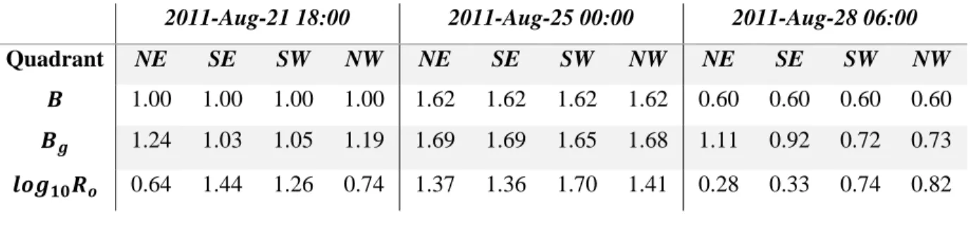
Figure 2.7 gives three snapshots of the radial wind profiles of Hurricane Irene (2011), at each of its developing, mature and dissipating stages, with a few parameters showing storm characteristics (Table 2.2). The left (right) three panels show cross-section winds from the SW to the NE (the NW to the SE) directions, and all specified isotachs (34, 50, and/or 64-knot) in the “best track” file are plotted in vertical bars at specified distances from the storm center, with the highest one in a dark color and the rest in gray. For a perfect match between the isotachs and the modeled winds, the tip of the vertical bars and the radial profiles must meet at the exact heights.
Table 2.2. Parameters of storm characteristics at three snapshots of Irene (2011)
2011-Aug-21 18:00 2011-Aug-25 00:00 2011-Aug-28 06:00
Quadrant NE SE SW NW NE SE SW NW NE SE SW NW
𝑩 1.00 1.00 1.00 1.00 1.62 1.62 1.62 1.62 0.60 0.60 0.60 0.60
𝑩𝒈 1.24 1.03 1.05 1.19 1.69 1.69 1.65 1.68 1.11 0.92 0.72 0.73
𝒍𝒐𝒈𝟏𝟎𝑹𝒐 0.64 1.44 1.26 0.74 1.37 1.36 1.70 1.41 0.28 0.33 0.74 0.82
the first snapshot), and all four quadrants in the second snapshot. When 𝑙𝑜𝑔10𝑅𝑜< 1, the AHM fails to match any highest isotach due to the issues detailed in section 2.2.1 (see the rest of the quadrants). Note that profiles by either the AHM or the GAHM tend to die off too quickly away from the storm center, and thus fail to match any lower isotach.
2.4.2 Evaluation of the RMW and the Modeled Maximum Wind
The time-series maximum wind and the corresponding RMW, which is the distance from storm center to the maximum wind found, were retrieved from the AHM, GAHM spatial wind snapshots for all seven storms. Comparison between the modeled and specified maximum winds in NHC’s “best track” files is shown in the upper two panels of Figure 2.8, with a simple linear regression computed for each panel. The colorbar represents the quadrant-averaged 𝑅𝑜 calculated in the GAHM in base 10 logarithmic scale. Results indicate that the GAHM has an excellent skill in estimating the maximum winds at all times, although overestimation of 𝑉𝑀can be found near the lower bound of the data. Careful examination of these over-estimates revealed that they were due to bad data entries in the “best track” file. This is particularly common for a weak but fast moving storm, and cautions should be taken when subtracting the storm’s translational speed from the specified maximum wind and isotachs, as the adjusted maximum wind might
2.5 Model Results using the Multiple-Isotach Approach
As demonstrated in section 2.4.1, a radial wind profile constructed by the GAHM using the single-isotach approach would only match the highest isotach instead of all isotachs, due to characteristics of the profile and limitations of this single-fitting method. In fact, underestimation of modeled winds at distances to isotachs other than the highest one was common, as the
computed wind profile tended to die off too quickly away from the storm center due to the nature of GAHM’s formulas. In an effort to minimize the combined error at distances to all available isotachs, and to improve the accuracy of the overall estimated wind field to a further spatial extent, the multiple-isotach approach, which is based on the composite wind method introduced in section 2.2.4, should be used whenever there is more than one isotach present in the best track file.
Figure 2.9. Three-dimensional snapshots of Irene’s radial wind profiles (left) and interpolated spatial wind field (right) by the single-isotach approach (upper two panels) and the multiple-isotach approach (lower two panels)
2.5.1 Evaluations of Composite Wind Fields
causing them to have quite distinctive spatial wind fields. In general, the calculated RMW in the AHM is closer to the storm center than in the GAHM, due to the cyclostrophic balance
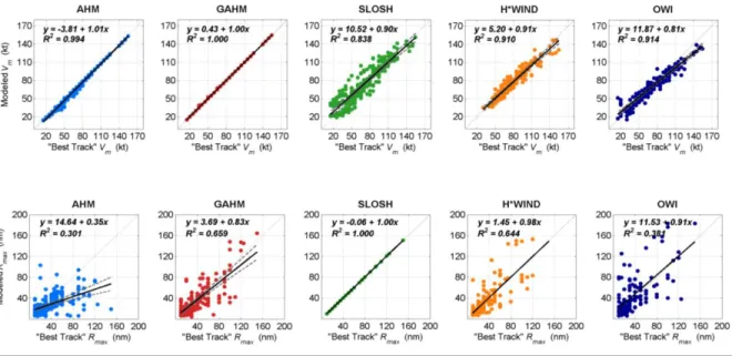
Evaluations of the modeled maximum wind and the RMW are shown in Figure 2.11. The distributions of the maximum winds identified in H*Wind, OWI winds, or SLOSH winds versus the specified maximum winds were rather dispersed, but the scatters is close to the 1:1 (dash) line, indicating a fairly good correlation, shown in upper panels. It is reasonable that the maximum winds reported in the “best track” advisories, which were approximated by
experienced forecasters based on limited information, naturally may not match the maximum winds perfectly in the re-analysis H*Wind and numerical OWI winds. Since the SLOSH model does not take the maximum winds as model input, the accuracy of its modeled maximum winds was not ideal here.
Figure 2.11. Comparison of the modeled and “Best Track” 𝑉𝑚 (upper five panels) and the modeled and “Best Track” 𝑅𝑚𝑎𝑥 (lower five panels) based on all seven hurricanes between the AHM, the GAHM, the SLOSH, the H*Wind and OWI winds.