Chapter 2_handout.pdf

(1)

CHAPTER 2

D

IRECT

M

ETHODS FOR

S

TOCHASTIC

S

EARCH

•Organization of chapter in ISSO

–Introductory material –Random search methods

•Attributes of random search •Blind random search (algorithm A)

•Two localized random search methods (algorithms B and C)

–Random search with noisy measurements

–Nonlinear simplex (Nelder-Mead) algorithm

•Noise-free and noisy measurements

Slides for Introduction to Stochastic Search and Optimization (ISSO) by J. C. Spall

Some Attributes of Direct Random Search

with Noise-Free Loss Measurements

• Three random search algorithms discussed in ISSO— algorithms A (blind random search), B, and C—share desirable attributes:

• Ease of programming

• Use of onlyLvalues (vs. gradient values)

– Avoid “artful contrivance” of more complex methods

• Reasonable computational efficiency • Generality

– Algorithms apply to virtually any function

• Theoretical foundation

(2)

2

2-3

Formal Convergence of Random

Search Algorithms

• Well-known results on convergence of random search

– Applies to convergence of and/or L

– Applies when noise-freeLmeasurements used in algorithms

• Algorithm A (blind random search) converges under very general conditions

– Applies to continuous or discrete functions

• Conditions for convergence of algorithms B and C somewhat more restrictive, but still quite general

– ISSOpresents theorem for continuous functions – Other convergence results exist

• Convergence ratetheory also exists: how fast to converge?

– Algorithm A generally slow in high-dimensional problems

2-4

Algorithm A:

Simple (“Blind”) Random Search

Step 0 (initialization) Choose an initial value of inside of . Set k= 0.

Step 1 (candidate value)Generate a new

independent value _new(k+1)  , according to the chosen probability distribution. If L(_new(k+1)) < set = _new(k+1). Else take

Step 2 (return or stop) Stop if maximum number ofL

evaluations has been reached or user is otherwise satisfied with the current estimate for ; else, return to step 1 with the new k set to the former k+1.

0

ˆ

  

ˆ

(

_k

),

L





ˆ

₁

(3)

2-5

First Several Iterations of Algorithm A on

Problem with Constraints and Quadratic

Loss Function (Example 2.1 in ISSO)

Iteration k new(k)

T

L(new(k)) ˆT_k L(ˆk)

0   [2.00, 2.00] 8.00

1 [2.25, 1.62] 7.69 [2.25, 1.62] 7.69

2 [2.81, 2.58] 14.55 [2.25, 1.62] 7.69

3 [1.93, 1.19] 5.14 [1.93, 1.19] 5.14

4 [2.60, 1.92] 10.45 [1.93, 1.19] 5.14

5 [2.23, 2.58] 11.63 [1.93, 1.19] 5.14

6 [1.34, 1.76] 4.89 [1.34, 1.76] 4.89

• Simple quadratic loss function L() = T_{on domain}₌ [1,3][1,3]

– Unique value = [1,1]T_with_L₍_{) = 2.0}

Global Convergence of Algorithm A

• Theorem 2.1 (Sect. 2.2 of ISSO) shows almost sure (a.s.) convergence of algorithm A to  under three key conditions

– Theorem uses concept of infimum(inf) of a function: greatest lower boundon specified domain

(4)

4

2-7

(a)Continuous L(); probability density for

newis > 0 on = [0, )

(b)Discrete L(); discrete sampling for _newwith P(_new= i) > 0 fori = 0, 1, 2,...

(c)Noncontinuous L(); probability density for _new is > 0 on  = [0, )



Functions for Convergence and

Nonconvergence of Algorithm A

(Blind Random Search)

• Functions that do ((a) and (b) below) or do not ((c) below) satisfy condition (2.2) of Theorem 2.1:

2-8

Algorithm B:

Localized Random Search

Step 0 (initialization) Choose an initial value of inside of . Set k= 0.

Step 1 (candidate value)Generate a random d_k. Check if

. If not, generate new d_kor move to nearest valid point. Let _new(k+1)  be or the modified point.

Step 2 (check for improvement) If L(_new(k+1)) < set = _new(k+1). Else take = .

Step 3 (return or stop) Stop if maximum number ofL

evaluations has been reached or if user satisfied with current estimate; else, return to step 1 with new kset to former k+1.

0 ˆ

  



ˆ

(

_k

),

L



ˆ ₁

k





ˆ

k

d

k



ˆ

k



d

k





ˆ

k

d

k





ˆ

₁

(5)

2-9

Comments on Algorithm B

• Algorithm B useful in many practical problems: easy to apply with reasonable efficiency when p> 1 (even p >> 1)

• Relative to algorithm A, search in algorithm B more localized in neighborhood of current estimate

– Better exploitation of information acquired about shape of L()

– “Localized” terminology not to be confused with global vs. local algorithms discussed in Chapter 1

• Algorithm B finds global optimum (“in probability”) per Theorem 2.2 in ISSO

• User free to set distribution of deviation vector d_k although

N(0,2_I

p) is most common in continuous problems

– Distribution should have mean zero and each component should have variation (e.g., standard deviation) consistent with magnitudes of corresponding components in 

• Often better if variability of d_k reduced as k increases

Algorithm C:

Enhanced Localized Random Search

• Similar to algorithm B

• Exploits knowledge of good/bad directions

• If move in one direction produces decreasein loss, add bias to next iteration to continuealgorithm moving in “good” direction

• If move in one direction produces increasein loss, add bias to next iteration to move algorithm in oppositeway

(6)

6

2-11

Examples 2.3 and 2.4 in ISSO:

Comparison of Algorithms A, B, and C

• Relatively simple p= 2 problem used elsewhere (Styblinski and Tang, 1990) to test simulated annealing algorithms

– Quartic loss function (plot on next slide)

• One global solution; several local minima/maxima

• Started all algorithms at common initial condition and compared based on common number of loss evaluations

– Algorithm A needed no tuning

– Algorithms B and C required “trial runs” to tune algorithm coefficients

(7)

2-13

Examples 2.3 and 2.4 in ISSO (cont’d):

Sample Means of Terminal Values

– L

(





)

in Multimodal Loss Function

(with Approximate 95% Confidence Intervals)

ˆ

(

_k

)

L



Notes:

Each sample mean is from 40 independent runs of relevant algorithm

Confidence intervals for algorithms B and C overlap slightly since 0.51 < 0.67

Examples 2.3 and 2.4 in ISSO (cont’d):

Typical Adjusted Loss Values ( – L

(





)

and Estimates of



in Multimodal

Loss Function (One Typical Run)



ˆ

(

_k

)

(8)

8

2-15

Random Search Algorithms with Noisy

Loss Function Measurements

• Basic implementation of random search above assumes perfect (noise-free) values of L

• Some applications require use of noisymeasurements:

y() = L() + noise

• Simplest modification is to form average of y values at each iteration as approximation to L

• Alternative modification is to set threshold > 0 for improvement before new value is accepted in algorithm • Thresholding in algorithm B with modified step 2:

Step 2 (modified) If y(_new(k+1)) < set = _new(k+1). Else take = .

• Very limited convergence theory with noisy measurements

– In fact, random search generally nonconvergentwith noisy loss measurements

 

ˆ

(

_k

)

,

y







ˆ

₁

k



ˆ

k1



ˆ

k

2-16

Nonlinear Simplex (Nelder-Mead) Algorithm

• Nonlinear simplex method is popular search method (e.g., fminsearch in MATLAB)

• Simplex is convex hullof p + 1 points in p

– Convex hull is smallest convex set enclosing the p + 1 points – Forp= 2 convex hull is triangle

– For p= 3 convex hull is pyramid

• Algorithm searches for  by moving convex hull within 

• If algorithm works properly, convex hull shrinks/collapses onto 

• No injected randomness (contrast with algorithms A, B, and C), but allowance for noisy loss measurements

(9)

2-17

Steps of Nonlinear Simplex Algorithm

Step 0 (Initialization) Generate initial set of p+ 1 extreme points in p_,i₍_i_{= 1, 2, …,}_p _{+ 1), vertices of initial simplex}

Step 1 (Reflection) Identify where max, second highest, and min loss values occur; denote them by _max, _2max, and _min, respectively. Let _cent = centroid (mean) of all i except for

_max. Generate candidate vertex _reflby reflecting _max through

_cent using _refl= (1 + )_cent   _max (> 0).

Step 2a (Accept reflection) If L(_min) L(_refl) < L(_2max), then

_reflreplaces _max; proceed to step 3; else go to step 2b.

Step 2b (Expansion) If L(_refl) < L(_min), then expand reflection using _exp= _refl+ (1  )_cent, > 1; else go to step 2c. If

L(_exp) < L(_refl), then _expreplaces _max; otherwise reject expansion and replace _max by _refl. Go to step 3.

Steps of Nonlinear Simplex Algorithm (cont’d)

Step 2c (Contraction) If L(_refl)  L(_2max), then contract simplex: Either case (i) L(_refl) < L(_max), or case (ii) L(_max) 

L(_refl). Contraction point is _cont= _max/refl+ (1  )_cent, 0  

 1, where _max/refl= _reflif case (i), otherwise _max/refl= _max. In case (i), accept contraction if L(_cont) L(_refl); in case (ii),

accept contraction if L(_cont) < L(_max). If accepted, replace

_maxby _contand go to step 3; otherwise go to step 2d.

Step 2d (Shrink) If L(_cont) L(_max), shrink entire simplex using a factor 0 <  < 1, retaining only _min. Go to step 3.

Step 3 (Termination) Stop if convergence criterion or

(10)

10

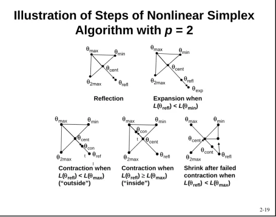
2-19

Illustration of Steps of Nonlinear Simplex

Algorithm with p = 2

Reflection

exp Expansion when

L(_refl) < L(_min)

max min

cent

refl

con t

max min

refl

cont

cent

2max

Contraction when

L(_refl) L(_max) (“inside”)

Shrink after failed contraction when

L(_refl) < L(_max)

con t

max min

cent

ref l

Contraction when

L(_refl) < L(_max) (“outside”)