Embodied Inference: or “I think therefore I am,
if I am what I think”
Karl Friston
Wellcome Trust Centre for Neuroimaging, London,
Institute of Neurology, University College of London, United Kingdom [email protected]
Introduction
This chapter considers situated and embodied cognition in terms of the free-energy principle. The free-energy formulation starts with the premise that biological agents must actively resist a natural tendency to disorder. It appeals to the idea that agents are essentially inference machines that model their sensorium to make predictions, which action then fulfils. The notion of an inference machine was articulated most clearly by Helm
-holtz1 and developed in psychophysics by Gregory2,3. The basic premise is that agents, and in particular their brains, entail a model of how their sensory data are generated. Optimization of this model’s parameters cor-responds to perceptual inference and learning on a moment to moment basis; while optimization of the model per se rests on changes in the form or configuration of the phenotype at neurodevelopmental or evolutionary timescales. The free-energy formulation generalises the concept of agents as inference machines and considers each agent as a statistical model of its environmental niche (econiche). In brief, the free-energy principle takes the existence of agents as its starting point and concludes that each pheno
-type or agent embodies an optimal model of its econiche. This optimality is achieved by minimizing free-energy, which bounds the evidence for each agent (model), afforded by sensory interactions with the world. In this sense, each agent distils and embodies causal structure in its local environment. However, the key role of embodiment also emerges in a slightly deeper and more subtle argument: Not only does the agent embody the environment but the environment embodies the agent. This is true in the sense that the physical states of the agent (its internal milieu) are part of the environment. In other words, the statistical model entailed by each agent includes a model of itself as part of that environment. This model rests upon prior expectations about how environmental states unfold over time. Crucially, for an agent to exist, its model must include the prior expectation that its form and internal (embodied) states are con-tained within some invariant set. This is easy to see by considering the alternative: If the agent (model) entailed prior expectations that it will change irreversibly, then (as an optimal model of itself), it will cease to
exist in its present state. Therefore, if the agent (model) exists, it must a priori expect to occupy an invariant set of bounded states (cf., homeosta-sis). Heuristically, if I am a model of my environment and my environ
-ment includes me, then I model myself as existing. But I will only exist iff (sic) I am a veridical model of my environment. Put even more simply;“I think therefore I am,4 iff I am what I think”. This tautology is at the heart of the free-energy principle and celebrates the circular causality that underpins much of embodied cognition.
Under this view, each organism represents a hypothesis or model that contains a different set of prior expectations about the environment it inhabits. Interactions with the environment can be seen as hypothesis testing or model optimisation, using the free-energy as a measure of how good its model is. Phenotypes or species that attain a low free-energy (i.e., maximise the evidence for their model) represent optimal solutions in a free-energy or fitness landscape, where exchanges with the environment are consistent with their prior expectations. The characteristic of biological agents is that they a priori expect their physical states to possess key inva-riance properties. These priors are mandated by the very existence of agents and lead naturally to phenomena like homeostasis, and preclude surprising exchanges with the world. It can be seen that the role of prior expectations is crucial in this formulation: If each agent is a hypothesis that includes prior expectations, then these expectations must include the prior that the agent occupies an invariant (attracting) set of physical states. However, this is only a hypothesis, which the agent must test using sensory samples from the environment. Iff its hypothesis is correct, the agent will retain its priors and maintain its states within physiological bounds. This highlights the key role of priors and their intimate relation
-ship to the structural form of phenotypes. It also suggests that simple prior expectations about homeostasis may be heritable and places the free-energy formulation (at least potentially) in an evolutionary setting. These arguments appeal to embodied cognition in that cognition and perception can be regarded as hypothesis testing about the environment in which the agent is situated, and which embodies the agent per se.
In summary, embodiment plays a fundamental and bilateral role in the free-energy formulation. On the one hand, agents embody (model) causal structure in the environment. On the other hand, the physical instantiation of this model is embodied in the environment. Only when the two are mutually compatible can the agent exist. This necessarily implies a low free-energy, which bounds the evidence for a model or hypothesis about an agent’s milieu. As the long-term average of negative log-evidence is the entropy of an agent’s sensory states, these low free-energy solutions implicitly resist a tendency to disorder and enable orga-nisms to violate the second law of thermodynamics.
and try to connect them to established theories about perception, cogni
-tion and behaviour. This chapter comprises three sec-tions. The first provides a heuristic overview of the free-energy formulation and its conceptual underpinnings. This formulation is inherently mathematical (drawing from statistical physics, dynamical systems and information theory). However, the basic ideas are intuitive and will be presented as such. For more technical readers, formal details (e.g., mathematical equa-tions) can be found in the figures and their legends. In the second section, we examine these ideas in the light of existing theories about how the brain works. In the final section, we will look more closely at the role of prior expectations as policies for negotiating with the environment and try to link policies to itinerancy and related concepts from synergetics.
1. The Free-Energy Principle
In recent years, there has been growing interest in applying free-energy principles to the brain5, not just in the neuroscience community, where it has caused some puzzlement6 but from fields as far apart as psycho -therapy7 and social politics8. The free-energy principle has been described as a unified brain theory9 and yet may have broader implications that speak to the way that any biological system interacts with its environ-ment. This section describes the origin of the free-energy formulation, its underlying premises and the implications for how we represent and interact with our world.
The free-energy principle is a simple postulate that has complicated ramifications. It says that self-organising systems (like us) that are at equi
-librium with their environment must minimise their free-energy10. This postulate is as simple and fundamental as Hamilton’s law of Least Action and the celebrated H-theorems in statistical physics. The principle was originally formulated as a computational account of perception that borrows heavily from statistical physics and machine learning. However, it quickly became apparent that its explanatory scope included action and behaviour and was linked to our very existence: In brief, the free-energy principle takes well-known statistical ideas and applies them to deep problems in population (ensemble) dynamics and self-organisation. In applying these ideas, many aspects of our brains, how we perceive and the way we act become understandable as necessary and self-evident attributes of biological systems.
The principle is essentially a mathematical formulation of how adap-tive systems (i.e., biological agents, like animals or brains) resist a natural tendency to disorder11-14. What follows is a non-mathematical treatment of its motivation and implications. We will see that although the motivation is quite straightforward, the implications are complicated and diverse. This diversity allows the principle to account for many aspects of brain
structure and function and lends it the potential to unify different perspectives on how the brain works. In the next section, we will see how the principle can be applied to neuronal systems, as viewed from these perspectives. This section is rather abstract and technical but the next section tries to unpack the basic idea in more familiar terms.
1.1 Resisting a tendency to disorder
The defining characteristic of biological systems is that they maintain their states and form in the face of a constantly changing environment11-14. From the point of view of the brain, the environment includes both the external and internal milieu. This maintenance of order is seen at many levels and distinguishes biological from other self-organising systems. Indeed, the physiology of biological systems can be reduced almost entirely to their homeostasis (the maintenance of physiological states within certain bounds15). More precisely, the repertoire of physiological and sensory states an organism can be in is limited, where those states define the organism’s phenotype. Mathematically, this means that the probability distribution of the agent’s (interoceptive and exteroceptive) sensory states must have low entropy. Low entropy just means that there is a high probability that a system will be in one of a small number of states, and a low probability that it will be in the remaining states. Entropy is also the average self-information. Self-information is the ‘surprise’ or improbability of something happening16 or, more formally, its negative log-probability. Here, ‘a fish out of water’ would be in a surprising state (both emotionally and mathematically). Note that both entropy and surprise depend on the agent; what is surprising for one agent (e.g., being out of water) may not be surprising for another. Bio
-logical agents must therefore minimise the long-term average of surprise to ensure that their sensory entropy remains low. In other words, bio
-logical systems somehow manage to violate the Fluctuation Theorem, which says the entropy of (non-adaptive) systems can fall but the probability of entropy falling vanishes exponentially as the observation time increases17.
In short, the long-term (distal) imperative, of maintaining states within physiological bounds, translates into a short-term (proximal) sup
-pression of surprise. The sort of surprise we are talking about here is asso
-ciated with unpredicted or shocking events (e.g., tripping and falling in the street or the death of a loved one). Surprise is not just about the current state (which cannot be changed) but also about the movement or transition from one state to another (which can). This motion can be very complicated and itinerant (wandering) provided it revisits a small set of states (called a global random attractor18) that are compatible with sur -vival (e.g., driving a car within a small margin of error). It is this motion or these state-transitions that the free-energy principle optimises.
So far, all we have said is that biological agents must avoid surprises to ensure that their exchanges with the environment remain within bounds. But how do they do this? A system cannot know whether its sensations are surprising or avoid them even if it did know. This is where free-energy comes in: Free-energy is an upper bound on surprise, which means that if agents minimise free-energy they implicitly minimise surpri
-se. Crucially, free-energy can be evaluated because it is a function of two things the agent has access to: its sensory states and a recognition density encoded by its internal states (e.g., neuronal activity and connection strengths).The recognition density is a probability distribution of putative environmental causes of sensory input; i.e., a probabilistic representation of what caused sensations. These causes can range from the presence of an object in the field of view that causes sensory impressions on the eye, to physiological states like blood pressure that cause interoceptive signals. The (variational) free-energy construct was introduced into statistical physics to convert difficult probability density integration problems into easier optimisation problems19. It is an information theoretic quantity (like surprise) as opposed to a thermodynamic energy. Variational free-energy has been exploited in machine learning and statistics to solve many inference and learning problems20-22. In this setting, surprise is called the (negative) model log-evidence (i.e., the log-probability of getting some sensory data, given it was generated by a particular model). In our case, the model is entailed by the agent. This means minimising surprise is the same as maximising the sensory evidence for a model or agent. In the present context, free-energy provides the answer to a fundamental question: How do self-organising adaptive systems avoid surprising states? They can do this by minimising their free-energy. So what does this involve?
1.2 Action and perception
In brief, agents can suppress energy by changing the two things free-energy depends on. They can change sensory input by acting on the world or they can change their recognition density by changing their internal states. This distinction maps nicely onto action and perception. One can understand this in more detail by considering three mathemati
-cally equivalent formulations of free-energy (see Fig. 1 and ref [5]; Supple
-mentary material, for a more formal treatment). The free-energy bound on surprise is constructed by simply adding a non-negative term to surprise. This term is a function of the recognition density encoded by the agent’s internal states. We will refer to this term as a posterior divergence. Creating the free-energy bound in this way leads to the first formulation:
1.2.1 Free-energy as posterior divergence plus surprise
The posterior divergence is a Kullback-Leibler divergence (cross entropy) and is just the difference between the recognition density and the poste-rior or conditional density on the causes of sensory signals. This conditio
-nal density represents the best possible guess about the true causes. The difference between the two densities is always non-negative and free-energy is therefore an upper bound on surprise. This is the clever part of the free-energy formulation; because minimising free-energy by changing the recognition density (without changing sensory data) reduces the diffe
-rence, making the recognition density a good approximation to the condi
-tional density and the free-energy a good approximation to surprise. The recognition density is specified by its sufficient statistics, which are the agent’s internal states. This means an agent can reduce posterior diver
-gence (i.e. free-energy) by changing its internal states. This is essentially perception and renders an agent’s internal states representations of the causes of its sensations.
1.2.2 Free-energy as prior divergence minus accuracy
The second formulation expresses free-energy as prior divergence minus accuracy. In the model comparison literature, prior divergence is called ‘complexity’. Complexity is the difference between the recognition density and the prior density on causes encoding beliefs about the state of the world before observing sensory data (this is also known as Bayesian surprise23). Accuracy is simply the surprise about sensations expected under the recognition density. This formulation shows that minimising free-energy by changing sensory data (without changing the recognition density) must increase the accuracy of an agent’s predictions. In short, the agent will selectively sample the sensory inputs that it expects. This is known as active inference24. An intuitive example of this process (when it is raised into consciousness) would be feeling our way in darkness; antici
-pating what we might touch next and then trying to confirm those expect
-ations. In short, agents can act on the world to minimise free-energy by increasing the accuracy of their predictions through selective sampling of the environment.
1.2.3 Free-energy as expected energy minus entropy
The final formulation expresses free-energy as an expected energy minus entropy. This formulation is important for three reasons. First, it connects the concept of free-energy as used in information theory with homologous concepts used in statistical thermodynamics. Second, it shows that the free-energy can be evaluated by an agent because the expected energy is the surprise about the joint occurrence of sensations and their perceived causes, while the entropy is simply the entropy of its recognition density. Third, it shows that free-energy rests upon a generative model of the
world; which is expressed in terms of the joint probability of a sensation and its causes occurring together. This means that an agent must have an implicit generative model of how causes conspire to produce sensory data. It is this model that defines both the nature of the agent and the qua
-lity of the free-energy bound on surprise.
1.3 Generative models in the brain
We have just seen that one needs a generative model (denoted by
p(s t%q( ) [ , , , ], ( | )ϑ µ|s s sm) in the figures) of how the sensorium is caused to evaluate free-energy. These models combine the likelihood of getting some data, given their causes and prior beliefs about these causes. These models have to explain complicated dynamics on continuous states with hierarchical or deep causal structure. Many biological systems, including the brain, may use models with the form shown in Fig. 2. These are hierarchical dynamic models and provide a very general description of states in the world. They are general in the sense that they allow for cascades or hierarchies of nonlinear dynamics to influence each other. They comprise equations of motion and static nonlinear functions that mediate the influence of one hierarchical level on the next. Crucially, these equations include random fluctuations on the states and their motion, which play the role of observa
-tion noise at the sensory level and state-noise at higher levels. These random fluctuations induce uncertainty about states of the world and the parameters of the model. In these models, states are divided into causal states, which link states in different hierarchical levels and hidden states, which link states over time and lend the model memory. Gaussian assumptions about the random fluctuations furnish the likelihood and (empirical) priors on predicted motion that constitute a probabilistic generative model. These assumptions about random effects are encoded by their (unknown) precision, or inverse variance. See Fig. 2 for details. We will appeal to this sort of model below, when trying to understand how the brain complies with the free-energy principle, in terms of its architecture and dynamics.
In summary, the free-energy induces a probabilistic model of how sensory data are generated and a recognition density on the model’s para-meters (i.e., sensory causes). Free-energy can only be reduced by changing the recognition density to change conditional expectations about what is sampled or by changing sensory samples (i.e. sensory input) so that they conform to expectations. This corresponds to perception and action respectively. We will see later that minimising free-energy corresponds to minimising prediction errors. It then becomes almost self-evident that bio-logical agents can suppress prediction errors by changing predictions (perception) or what is predicted (action): see Fig. 2. In the next section, we consider the implications of this formulation in light of some key theories about the brain.
Fig. 1: The free-energy principle. This schematic shows the dependencies among the quan-tities that define the free-energy of an agent or brain, denoted by m. These include, its internal states µ(t), generalised sensory signals (i.e., position, velocity, acceleration etc.)
( ) [ , , , ]
s t% (t) = [s s ss, s’, s’’, ...]T and action α(t). The environment is described by equations, which specify the motion of its states {x(t), ν(t)}. Both internal brain states and action minimise free-energy F (s t%( ) [ , , , ], µ), which is a function of sensory input and the internal states. These states encode a s s s
recognition density q(q( | )ϑ µ| µ) on the causes q( | )ϑ µ⊃ { x, ν, θ, γ} of sensory input. These comprise states of the world u(t) : u ∈ x, ν and parameters φ∈θ, γ controlling the equations of motion and the amplitude of the random fluctuations ω(u) : u ∈ x, ν on the hidden states and sensory input. The lower panel provides the key equations behind the free-energy formulation. The first pair says that the path integral of free-energy (free-action; S) is an up-per bound on the entropy of sensory states, H. This entropy is average surprise, which (under ergodic assumptions) is the long-term average or path integral of surprise. The free-energy per se F (t):= F (s t%( ) [ , , , ], µ) is then expressed in three ways to show what its minimisation s s s
means. The first equality shows that optimising brain states, with respect to the internal states, makes the recognition density an approximate conditional density on the causes of sensory input. Furthermore, it shows that free-energy is an upper bound on surprise. This enables action to avoid surprising sensory encounters. The second equality shows that action can only reduce free-energy by selectively sampling data that are predicted by under the recognition density. The final equality expresses free-energy in terms of an expected energy L (t) based on a generative model and the entropy Q(t) of the recognition density. In this fi-gure, < · >q denotes expectation or average, under the recognition density and DKL (· || ·) is a non-negative Kullback-Leibler divergence (i.e., difference between two probability densi-ties). In summary, free-energy rests on two probability densities; one that generates sensory samples and their causes, p(s t%q( ) [ , , , ], ( | )ϑ µ| ms s s) and the recognition density, qq(( | )ϑ µ| µ). The first is a pro-babilistic generative model, whose form is entailed by the agent or brain (denoted by m), while the second represents the best probabilistic estimate of the causes and is encoded by internal states. The free-energy principle states that all quantities that can change (sufficient statistics and action) minimise free-energy.
Fig. 2 (next page): Action and perception. This schematic illustrates the bilateral role of free-energy (i.e., prediction error) in driving action and perception: Action: Acting on the envi-ronment by minimising free-energy enforces a sampling of sensory data that is consistent with the current representation (i.e., changing sensations to minimise prediction error). This
is because free-energy is a mixture of complexity and accuracy (the second expression for free-energy in Fig. 1). Crucially, action can only affect accuracy. This means the brain will reconfigure its sensory epithelia to sample inputs that are predicted by its representations; in other words, to minimise prediction errors. The equation above action simply states that ac-tion performs a gradient decent on (i.e., minimises) free-energy (see ref [10] for details). Per-ception: Optimizing free-energy by changing the internal states that encode the recognition density makes it an approximate posterior or conditional density on the causes of sensations. This follows because free-energy is surprise plus a Kullback-Leibler divergence between the recognition and conditional densities (the first expression for free-energy in Fig. 1). Because this difference is non-negative, minimising free-energy makes the recognition density an approximate posterior probability. This means the agent implicitly infers or represents the causes of its sensory samples in a Bayes-optimal fashion. At the same time, the free-energy becomes a tight bound on surprise that is minimised through action. The equation above perception simply states that internal states perform a gradient decent on (i.e., minimise) free-energy. This gradient decent is in a moving frame of reference for generalised states and accumulates gradients over time for the parameters (see ref [5] for details). Prediction error: Prediction error is simply the difference between predicted and observed sensory states. The equations show that the free-energy comprises the expected energy L (t), which is effectively the (precision weighted) sum of squared error. This error contains the sensory prediction error and other differences that mediate empirical priors on the motion of hidden states and the parameters. The predictions rest on a generative model of how sensations are caused. These models have to explain complicated dynamics on continuous states with hierarchical or deep causal structure. An example of one such generic model is shown on the right. Generative model: Here ƒ(i,u) : u ∈ x, ν are continuous nonlinear functions of (hidden and causal) states, parameterised by θq⊂( | )ϑ µ at the i-th level of a hierarchical dynamic model. The random fluctuations ω(u) : u ∈ x, ν play the role of observation noise at the sensory level and state-noise at higher levels. Causal states ν(i)q⊂( | )ϑ µ link hierarchical levels, where the output of one level provides input to the next. Hidden states x(i)q⊂( | )ϑ µlink dynamics over time and lend the model memory. Gaussian assumptions about the random fluctuations specify the likelihood and furnish empirical priors in terms of predicted motion. These assumptions are encoded by their or precision or inverse variance Π(i,u) : u ∈ x, ν, which depend on precision parameters γq⊂( | )ϑ µ. The associated message-passing scheme implementing perception is shown in the next figure. In this and subsequent figures, subscripts denote differentiation, D is a temporal derivative operator that acts on generalised states and κ is a large positive con-stant (see ref [48] for details).
THE BAYESIAN BRAIN AND OTHER THEORIES
This section attempts to place some key brain theories within the free-energy framework, in the hope of identifying common themes. It reprises and extends the review in ref [5]. We will consider a range of theories that derive from both the biological and physical sciences (e.g., neural Darwinism, information theory and optimal control). Crucially, one key theme runs throughout these theories; namely, optimization. Further-more, if we look closely at what is optimized, the same quantity keeps emerging, namely value, expected reward, expected utility; or its com-plement: surprise, prediction-error or expected cost. We will see that this quantity is effectively free-energy.
2.1 The Bayesian brain hypothesis
The Bayesian brain hypothesis25 uses Bayesian probability theory to for-mulate perception as a constructive process based on internal or genera-tive models. The underlying idea is that the brain has a model of the world1-3 that it tries to optimise using sensory inputs28-33. This idea is related to analysis by synthesis27 and epistemological automata26. In other words, the brain is an inference machine that actively predicts and explains its sensations1,3,30. Central to this hypothesis is a probabilistic model that can generate predictions, against which sensory samples are tested to update beliefs about their causes. In Bayesian treatments, this generative model decomposes into the likelihood (the probability of sen-sory data, given their causes) and a prior (the a priori probability of those causes). Perception then becomes the inversion of the likelihood model (mapping from causes to sensations) to access the posterior probability of the causes, given sensory data (mapping from sensations to causes). This inversion is exactly the same as minimising the difference between the recognition and posterior densities (posterior divergence) to suppress free-energy. Indeed, the free-energy formulation was developed to finesse the difficult problem of exact inference by converting it into an easier optimisation problem19-22. This has furnished some powerful approxima-tion techniques for model identificaapproxima-tion and comparison (e.g., variaapproxima-tional Bayes or ensemble learning34). There are many interesting issues that attend the Bayesian brain hypothesis; we will focus on two.
The first is the form of the generative model and how it manifests in the brain. One criticism of Bayesian treatments is that they ignore the question of how prior beliefs, which are necessary for inference, are formed32. However, this criticism disappears under hierarchical genera-tive models, in which the priors themselves are optimised31,33. In hierar-chical models (cf, the right panel in Fig. 2), causes in one level of a model generate subordinate causes in a lower level, while the sensory data per se
are generated at the lowest level. Minimising the free-energy of represen-tations effectively optimises empirical priors (i.e., the probability of causes at one level, given those in the level above). Crucially, because empirical priors are linked hierarchically, they are informed by sensory data, enabling the brain to optimise its prior expectations online. This optimi-sation makes every level in the hierarchy accountable to others, furnishing an internally consistent representation of sensory causes, at multiple levels of description. Not only do hierarchical models have a key role in statistics (e.g., random effects models and parametric empirical Bayes35,36), they may also be an important metaphor for the brain, given the hierar-chical arrangement of its cortical sensory areas37-39.
The second issue is the form of the recognition density. This has to be encoded by physical attributes (i.e., internal states) of the brain, such as synaptic activity, efficacy and gain. In general, any density is encoded by its sufficient statistics (for example, the mean and variance of a Gaussian density). The way the brain encodes these statistics places important constraints on the sorts of schemes that underlie recognition. The dif-ferences between these schemes can usually be reduced to difdif-ferences in the form of the recognition density. They range from free-form schemes, which use a vast number of sufficient statistics (e.g., particle filtering31 and
probabilistic population codes40-43) to simpler forms, which make stronger assumptions about the shape of the recognition density. These assump-tions mean that the recognition density can be encoded with a small num-ber of sufficient statistics. The simplest assumed form is Gaussian, which only requires the conditional mean or expectation. This is also known as the Laplace assumption 44, under which the free-energy reduces to the sum of squared prediction error at each level of the model (in fact, this assumption gives exact inference under some common models, such as factor analysis45). Minimising free-energy then corresponds to explaining away the prediction error (Fig. 2). This is known as predictive coding and has become a popular framework for understanding neuronal message-passing among different levels of sensory cortical hierarchies46. In this scheme, prediction error units compare conditional expectations with top-down predictions to elaborate a prediction error. This is passed forward to drive the units in the level above that encode conditional expectations and optimise top-down predictions to explain (i.e., reduce) prediction error in the level below. This just means countering excitatory bottom-up inputs to a prediction error neuron with inhibitory synaptic inputs that are driven by top-down predictions. See Fig. 3 and refs [47] and [48] for a detailed discussion. The reciprocal exchange of bottom-up prediction errors and top-down predictions proceeds until prediction error is minimised at all levels and conditional expectations are optimised. This scheme has been invoked to explain many features of early visual respon-ses 46,49 and provides a plausible account of repetition suppression and
mismatch responses in electrophysiology50. Fig. 4 provides an example of perceptual categorisation that uses this scheme. Message-passing of this sort is consistent with known functional asymmetries in real cortical hierarchies 51, where forward connections (which convey prediction errors) are driving and backwards connections (that model the nonlinear generation of sensory input) show both driving and modulatory characte-ristics 52. This asymmetric message-passing is also a characteristic feature of adaptive resonance theory53,54, which shares formal similarities with predictive coding.
In summary, the theme underlying the Bayesian brain and predictive coding is that the brain is an inference engine that is trying to optimise probabilistic representations of what caused its sensory input. This opti-misation can be finessed using a (variational free-energy) bound on sur-prise. In machine learning and statistics, surprise is known as the (nega-tive) log-evidence or marginal likelihood of some data, given a model. In this sense, the free-energy principle subsumes the Bayesian brain hypothesis and can be implemented by the many schemes considered in this field. Almost invariably, these involve some form of message-passing or belief propagation among brain areas or units. We have focused on one of the simplest schemes, namely predictive coding, which lends itself to a neurobiologically plausible implementation. Furthermore, it allows us to connect to another principled approach to sensory processing, namely information theory:
2.2 The principle of efficient coding
This principle suggests that the brain optimises the mutual information (i.e., mutual predictability) between the sensorium and its internal repre-sentation, under constraints on the efficiency of those representations. This line of thinking was articulated by Barlow55 in terms of a redundancy reduction principle (or principle of efficient coding) and formalised later in terms of the infomax principle56. It has been applied in machine learning57, leading to things like independent component analysis58, and in neurobiology, to understand the nature of neuronal responses59-62. This principle is extremely effective in predicting the empirical characteristics of classical receptive fields59 and provides a formal explanation for sparse coding61 and the segregation of processing streams in visual hierarchies63. It has been extended to cover dynamics and motion trajectories64,65 and even used to infer the metabolic constraints on neuronal processing66. At its simplest, it says that neuronal activity should encode sensory informa-tion in an efficient and parsimonious fashion. It considers the mapping between one set of variables (sensory states) and another (variables repre-senting those states). At first glance, this seems to preclude a probabilistic representation, because this would involve a mapping between sensory states and a probability density. However, the infomax principle can be
applied to the sufficient statistics of a recognition density. In this context, the infomax principle suggests that conditional expectations should afford an accurate but parsimonious prediction of sensory signals.
Crucially, the infomax principle is a special case of the free-energy principle, which arises when we ignore uncertainty in probabilistic repre-sentations (and when there is no action, see Fig. 5 and ref [5]; supplemen-tary material for mathematical details). This is easy to see by noting that sensory signals are generated by causes. This means it is sufficient to represent the causes to predict these signals. More formally, the infomax principle can be understood in terms of the decomposition of free-energy into complexity and accuracy: Mutual information is optimised when con-ditional expectations maximise accuracy (or minimise prediction error), while efficiency is assured by minimising complexity (the prior diver-gence). This ensures that the generative model is not over-parameterised and leads to a parsimonious representation of sensory data that conforms to prior constraints on their causes. It is interesting that advanced model optimisation techniques use free-energy optimisation to eliminate redun-dant model parameters67. This might provide a nice explanation for synaptic pruning and homeostasis in the brain during neurodevelop-ment68 and sleep69.
The infomax principle pertains to a forward mapping from sensory input to representations. How does this relate to optimising generative models, which map from causes to sensory inputs?These perspectives can be reconciled by noting that all recognition schemes based on infomax can be cast as optimising the parameters of a generative model70. For example, in sparse coding models61, the implicit priors posit independent causes that are sampled from a heavy tailed or sparse distribution48. The fact that these models predict empirically observed receptive fields so well, suggests that we are endowed with (or acquire) prior expectations that the causes of our sensations are largely independent and sparse.
Bayesian surprise was invoked recently to explain sampling in models of visual search and salience23. Bayesian surprise is the difference between the posterior and prior densities on the causes of sensory input and is formally identical to complexity. It is interesting because it appears to contradict the principle of efficient coding; in that maximising Bayesian surprise increases complexity. However, this apparent paradox is resolved easily by noting that any change to the posterior (or recognition) density that increases accuracy will incur a complexity cost and increase Bayesian surprise. However, under the free-energy formulation, Bayesian surprise per se is not optimised; it should be minimised in the absence of a recognisable stimulus. It might be interesting to test this prediction empirically.
Fig. 3: Hierarchical message-passing in the brain. The schematic details a neuronal architecture that optimises the conditional expectations of causes in hierarchical models of sensory input of the sort illustrated in the previous figure. It shows the putative cells of origin of forward driving connections that convey prediction-error from a lower area to a higher area (grey arrows) and nonlinear backward connections (black arrows) that construct predictions 47. These predictions try to explain away prediction-error in lower levels. In this scheme, the sources of forward and backward connections are superficial and deep pyramidal cells (triangles) respectively, where state-units are black and error-units are grey. The equations represent a gradient descent on free-energy using the generative model of the previous figure. Predictions and prediction-error: If we assume that neuronal activity encodes the conditional expectation of states, then recognition can be formulated as a gradient descent on free-energy. Under Gaussian assumptions, these recognition dynamics can be expressed compactly in terms of precision weighted prediction-errors ξ(i,u) : u ∈ x, ν on the causal states and motion of hidden states. The ensuing equations suggest two neuronal populations that exchange messages; causal or hidden state-units encoding expected states and error-units encoding prediction-error. Under hierarchical models, error-units receive messages from the state-units in the same level and the level above; whereas state-units are driven by error-units in the same level and the level below. These provide bottom-up messages that drive conditional expectations µ(i,u) : u ∈ x, ν towards better predictions to explain away prediction-error. These top-down predictions correspond to ƒ(i,u) : u ∈ x, ν. This scheme suggests the only connections that link levels are forward connections conveying prediction-error to state-units and reciprocal backward connections thatmediate predictions. Note that the prediction errors that are passed forward are weighted by their precision. This tells us that precision may be encoded by the postsynaptic gain or sensitivity of error units, which also has to be optimised: Synaptic plasticity and gain: The corresponding equations for changes in the conditional expectation of the parameters of the model and the precisions of random fluctuations are related to formal models of associative plasticity and reinforcement learning: see refs [48] and [146] for further details.
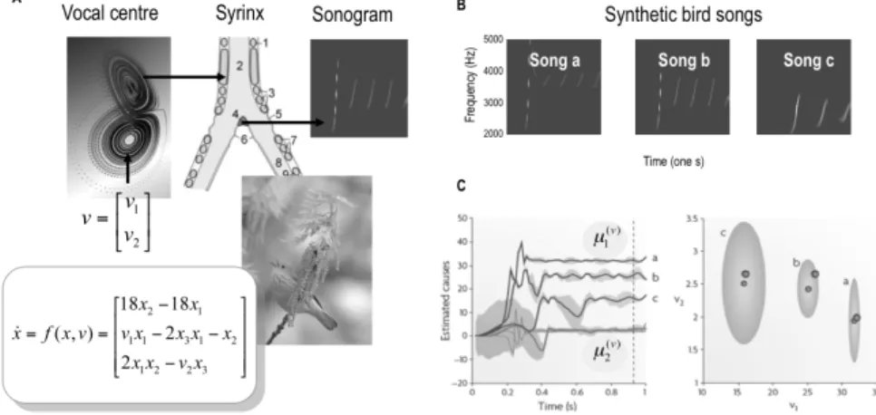
Fig. 4 (next page): Birdsongs and perceptual categorisation. Left: The generative model of birdsong used in this simulation comprises a Lorenz attractor, whose shape is determined by two causal states (ν1 ,ν2). Two of the attractor’s hidden states are used to modulate the am-plitude and frequency of stimuli generated by a synthetic syrinx (an example is shown as a sonogram). The ensuing stimuli were then presented to a synthetic bird to see if it could recover the causal states (ν1 ,ν2) that categorise the chirp in a two-dimensional perceptual
space. This involves minimising free-energy by changing the internal representation (µ1(ν) ,µ2(ν)) of the causes. Examples of this perceptual inference or categorisation are shown on the right. Right: Three simulated songs are shown (upper panels) in sonogram format. Each comprises a series of chirps whose frequency and number fall progressively (from a to c), as a causal state (known as the Raleigh number; ν1 on the left) is decreased. Lower left: This graph depicts the conditional expectations of the causal states, shown as a function of peristimulus time for the three songs. It shows that the causes are identified after about 600 milliseconds with high conditional precision (90% confidence intervals are shown in grey). Lower right: This shows the conditional density on the causes shortly before the end of peristimulus time (i.e., the dotted line in the left panel). The small dots correspond to condi-tional expectations and the grey areas correspond to the 90% condicondi-tional confidence regions. Note that these encompass the true values (large dots) used to generate the songs. These results illustrate the nature of perceptual categorisation under the inference scheme in Fig. 3: Here, recognition corresponds to mapping from a continuously changing and chaotic sensory input to a fixed point in perceptual space.
Fig. 5: Free-energy and info-max. This schematic provi-des the key equalities that show the infomax principle is a special case of the free-energy principle that ob-tains when we discount un-certainty and represent sen-sory data with point estima-tes of their causes. Alterna-tively, the free-energy is a generalization of the info-max principle that covers probability densities on the unknown causes of data. Horace Barlow and Ralph Linsker are two of the key people behind the principle of efficient coding and info-max.
In summary, the principle of efficient coding says the brain should optimise the mutual information between its sensory signals and some parsimonious neuronal representations. This is the same as optimising the parameters of a generative model to maximise the accuracy of predictions (i.e., to minimise prediction error), under complexity constraints. Both are mandated by the free-energy principle, which can be regarded as a pro-babilistic generalisation of the Infomax principle (see Fig. 5). We now turn to more biologically inspired ideas about brain function that focus on neuronal dynamics and plasticity. This takes us deeper into neurobio-logical mechanisms and implementation of theoretical principles above.
2.3 The cell assembly and correlation theory
The cell assembly theory was proposed by Hebb71 and entails Hebbian ― or associative ― plasticity, which is a cornerstone of neural network theory and of the empirical study of use-dependent or experience-depen-dent plasticity72. There have been several elaborations of this theory; for example, the correlation theory of von der Malsburg73,74 and formal refi-nements to Hebbian plasticity per se75. The cell assembly theory posits the formation of groups of interconnected neurons through a strengthening of their synaptic connections that depends on correlated pre- and post-synaptic activity; i.e., ‘cells that fire together wire together’. This enables the brain to distil statistical regularities from the sensorium. The correla-tion theory considers the selective enabling of synaptic efficacy and their plasticity (cf. meta-plasticity76) by fast synchronous activity induced by different perceptual attributes of the same object (e.g., a red bus in motion). This resolves a putative deficiency of classical plasticity, which cannot ascribe a pre-synaptic input to a particular cause (i.e., redness of the bus)73. The correlation theory underpins theoretical treatments of syn-chronised brain activity and its role in associating or binding attributes to specific objects or causes74,77. Another important field that rests upon associative plasticity is the use of attractor networks as models of memory formation and retrieval78-80. So how do correlations and associative pla-sticity figure in the free-energy formulation?
Hitherto, we have considered only inference on states of the world that cause sensory signals, where conditional expectations about states are encoded by synaptic activity. However, the causes covered by the recog-nition density are not restricted to time-varying states (e.g., the motion of an object in the visual field); they also include time-invariant regularities that endow the world with causal structure (e.g., objects fall with constant acceleration). These regularities are parameters of the generative model and have to be inferred by the brain. The conditional expectations of these parameters may be encoded by synaptic efficacy (these expectations are µ(θ) in Fig. 3). Inference on parameters corresponds to optimising connec-tion strengths in the brain; i.e., plasticity that underlines learning. So what
form would this learning take? It transpires that a gradient descent on free-energy (i.e., changing connections to reduce free-energy) is formally identical to Hebbian plasticity33,48 (see Fig. 3). This is because the para-meters of the generative model determine how expected states (synaptic activity) are mixed to form predictions. Put simply, when the pre-synaptic predictions and post-synaptic prediction-errors are highly correlated, the connection strength increases, so that predictions can suppress prediction errors more efficiently. Fig. 6 shows a simple example of this sort of sen-sory learning, using an oddball paradigm to elicit repetition suppression.
In summary, the formation of cell assemblies reflects the encoding of causal regularities. This is just a restatement of cell assembly theory in the context of a specific implementation (predictive coding) of the free-energy principle. It should be acknowledged that the learning rule in predictive coding is really a delta rule, which rests on Hebbian mechanisms; however, Hebb's wider notions of cell assemblies were formulated from a non-statistical perspective. Modern reformulations suggest that both infe-rence on states (i.e., perception) and infeinfe-rence on parameters (i.e., learn-ing) minimise free-energy (i.e., minimise prediction error) and serve to bound surprising exchanges with the world. So what about synchronisa-tion and the selective enabling of synapses?
2.4 Biased competition and attention
To understand what is represented by the modulation of synaptic efficacy
― or synaptic gain ― we have to consider a third sort of cause in the envi-ronment; namely, the amplitude of random fluctuations. Causal regulari-ties encoded by synaptic efficacy control the deterministic evolution of states in the world. However, stochastic or random fluctuations in these states play an important part in generating sensory data. Their amplitude is usually parameterized as precision (i.e., inverse variance) that encodes the reliability of prediction errors. Precision is important, especially in hierarchical schemes, where it controls the relative influence of bottom-up prediction errors and top-down predictions. So how is precision encoded in the brain? In predictive coding, expected precision modulates the amplitude of prediction errors (these expectations are µ(γ) in Fig. 3), so that prediction errors with high precision have a greater impact on units enco-ding conditional expectations. This means that precision corresponds to the synaptic gain of prediction error units. The most obvious candidates for controlling gain (and implicitly encoding precision) are classical neuromodulators like dopamine and acetylcholine, which provides a nice link to theories of attention and uncertainty81-83. Another candidate is fast synchronised pre-synaptic input that lowers effective post-synaptic mem-brane time constants and increases synchronous gain84. This fits com-fortably with the correlation theory and speaks to recent ideas about the role of synchronous activity in mediating attentional gain85,86.
In summary, the optimisation of expected precision in terms of synaptic gain links attention and uncertainty in perception (through balancing top-down and bottom-up effects on inference) to synaptic gain and synchronisation. This link is central to theories of attentional gain and biased competition86-91, particularly in the context of neuromodulation92,93. Clearly, these arguments are heuristic but show how different perspec-tives can be linked by examining mechanistic theories of neuronal dynamics and plasticity under a unifying framework. Fig. 7 provides a summary of the various neuronal processes that may correspond to opti-mising conditional expectations about states, parameters and precisions; namely, optimising synaptic activity, efficacy and gain respectively. In cognitive terms, these processes map nicely onto perceptual inference, learning and attention. The theories considered so far have dealt only with perception. However, from the point of view of the free-energy principle, perception just makes free-energy a good proxy for surprise. To actually reduce surprise we need to act. In the next section, we retain a focus on cell assemblies but move to the selection and reinforcement of stimulus-response links.
2.5 Neural Darwinism and value-learning
In the theory of neuronal group selection94, the emergence of neuronal assemblies or groups is considered in the light of selective pressure. The theory has four elements: Epigenetic mechanisms create a primary reper-toire of neuronal connections, which are refined by experience-dependent plasticity to produce a secondary repertoire of neuronal groups. These are selected and maintained through reentrant signalling (the recursive exchange of signals among neuronal groups). As in cell assembly theory, plasticity rests on correlated pre and post-synaptic activity but here it is modulated by value. Value is signalled by ascending neuromodulatory transmitter systems and controls which neuronal groups are selected and which are not. The beauty of neural Darwinism is that it nests selective processes within each other. In other words, it eschews a single unit of selection and exploits the notion of meta-selection (the selection of selec-tive mechanisms; e.g. ref [95]). In this context, value confers adapselec-tive fitness by selecting neuronal groups that meditate adaptive stimulus-stimulus associations and stimulus-stimulus-response links. The capacity of value to do this is assured by natural selection; in the sense that neuronal systems reporting value are themselves subject to selective pressure.
This theory, particularly value-dependent learning96, has deep connections with reinforcement learning and related approaches in engineering such as dynamic programming and temporal difference models97,98 (see below). This is because neuronal systems detecting valuable states reinforce connections to themselves, thereby enabling the brain to label a sensory state as valuable iff it leads to another valuable
state. This ensures that agents move through a succession of states that have acquired value to access states (rewards) with genetically specified (innate) value. In short, the brain maximises value, which may be reflected in the discharge of dedicated neuronal systems (e.g., dopami-nergic systems98-102). So how does this relate to the optimisation of free-energy?
The answer is simple: value is inversely proportional to surprise, in the sense that the probability that a phenotype is in a particular state increases with the value of that state. More formally V = -Г ln p(s t%( ) [ , , , ]| m), s s s where Г encodes the amplitude of random fluctuations (see ref [5];
sup-plementary material). This means the adaptive fitness of a phenotype is the negative surprise averaged over all the states it experiences, which is simply its negative entropy. Indeed, the whole point of minimising free-energy (and implicitly entropy) is to ensure agents spend most of their time in a small number of valuable states. In short, that free-energy is (a bound on) the complement of value and its long-term average is (a bound) on the complement of adaptive fitness. But how do agents know what is valuable? In other words, how does one generation tell the next which states have value (i.e., are unsurprising). Value or surprise is determined by the agent’s generative model and its implicit expectations
― these specify the value of sensory states and, crucially, are heritable. This means prior expectations that are specified epigenetically can prescribe an attractive state. In turn, this enables natural selection to optimise prior expectations and ensure they are consistent with the agent’s phenotype. Put simply, valuable states are just states the agent expects to frequent. These expectations are constrained by the form of its generative model, which is specified genetically and fulfilled beha-viourally, under active inference. It is important to appreciate that prior expectations include not just what will be sampled from the world but how the world sampled. This means natural selection may equip agents with the prior expectation they will explore their environment, until attractive states are encountered. We will look at this more closely in the next section, where priors on motion through state-space are cast in terms of policies in reinforcement learning.
In summary, neuronal group selection rests on value, which depends on prior expectations about what agents expect to encounter. These expec-tations are sensitive to selective pressure at an evolutionary timescale and are fulfilled as action minimises free-energy. Both Neural Darwinism and the free-energy principle try to understand somatic changes in an indivi-dual in the context of evolution: Neuronal Darwinism appeals to selective processes, while the free-energy formulation considers the optimisation of ensemble or population dynamics in terms of entropy and surprise. The key theme that emerges here is that (heritable) prior expectations can label things as innately valuable (unsurprising); but how does labelling states
lead to adaptive behaviour? In the final section, we return to reinfor-cement learning and related formulations of action that try to explain adaptive behaviour in terms of policies and cost-functions.
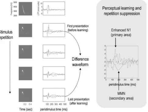
Fig. 6: A demonstration of perceptual learning. This figure shows the results of a simulated roving oddball paradigm, in which a stimulus is changed sporadically to elicit an oddball (i.e., deviant) response. The stimuli used here are chirps of the same sort as those used in Fig. 4. Left panels: The left column shows the percepts elicited in sonogram format. These are simply the predictions of sensory input, based on their inferred causes (i.e., the expecta -tions about hidden states). The right column shows the evolution of prediction error at the first (dotted lines) and second (solid line) levels of a simple linear convolution model (in which a causal state produces time-dependent amplitude and frequency modulations). The results are shown for one learned chirp (top graph) and the first four responses to a new chirp (lower graphs). The new chirp was generated by changing the parameters of the underlying equations of motion. It can be seen that following the first oddball stimulus, the prediction errors show repetition suppression (i.e., the amplitudes of the traces get smaller). This is due to learning the model parameters over trials (see synaptic plasticity and gain in Fig. 3). Of particular interest is the difference in responses to the first and last presentations of the new stimulus: these correspond to the deviant and standard responses, respectively. Right panel: This shows the difference between standard and oddball responses, with an enhanced negativity at the first level early in peristimulus time (dotted lines for inferred amplitude and frequency), and a later negativity at the higher or second level (solid line for the causal state). These differences could correspond to phenomena like enhanced N1 effects and the mismatch negativity (MMN) found in empirical difference waveforms. Note that superficial pyramidal cells (see Fig. 3) dominate event related potentials and that these cells may encode prediction error47,146.
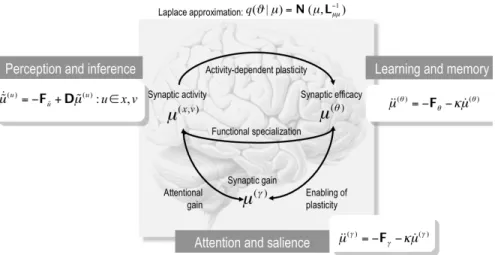
Fig. 7: The recognition density and its sufficient statistics. This schematic maps free-energy optimisation of the recognition density to putative processes in the brain: Under the Laplace assumption, the sufficient statistics of the recognition density (encoded by internal states) reduce to the conditional expectations (i.e., means). This is because the conditional precision is the curvature of the energy evaluated at the mean. Optimizing the conditional means of states of the world may correspond to optimising synaptic activity that mediates hierarchical message passing. Optimising the conditional means of parameters encoding causal structure may be implemented by associative mechanisms implementing synaptic plasticity and, finally, optimizing the conditional precisions may correspond to optimising synaptic gain (see Fig. 3).
POLICIES AND PRIORS
So far, we have established a fundamental role for generative models in furnishing a free-energy bound on surprise (or the value of attracting states an agent occupies). We have considered general (hierarchical and dynamic) forms for this model that prescribe predictions about how an agent will move through its state-space: in other words the state-transi-tions it expects. This expected motion corresponds to a policy that action is enslaved to pursue. However, we have not considered the form of this policy; i.e., the form of the equations of motion. In this section, we will look at universal forms for policies that define an agent’s generative model. Because policies are framed in terms of equations of motion they manifest as (empirical) priors on the state-transitions an agent expects to make. This means that policies and priors are the same thing (under active inference) and both rest on the form of generative models embodied by agents. We first consider universal forms based on optimal control theory and reinforcement learning. These policies use an explicit representation of value to guide motion, under simplifying assumptions about state-transitions. Although useful heuristics these policies do not generalise to
dynamical settings. This is because they only lead to fixed (low-cost) states (i.e., fixed-point attractors). Although this is fine for plant control in engineering or psychology experiments with paradigmatic end-points, fixed-point policies are not viable solutions for real agents (unless they aspire to be petrified or dead). We will then move on to wandering or itinerant policies that lead to invariant sets of attracting states. Itinerant policies may offer universal policies and implicitly, universal forms for generative models.
From the previous section, policies (equations of motion in Fig. 2) have to satisfy constraints that are hereditable. In other words, they have to be elaborated given only sparsely encoded information about what states are innately attractive or costly, given the nature of the agent’s phe-notype. We will accommodate this with the notion of cost-functions. Cost-functions can be thought of as standing in for the genetic specification of attractive states but they also allow us to connect to another important perspective on policies from engineering and behavioural economics:
3.1 Optimal control and Game Theory
Value is central to theories of brain function that are based on reinforce-ment learning and optimum control. The basic notion that underpins these treatments is that the brain optimises value, which is expected reward or utility (or its complement, expected loss or cost). This is seen in behavioural psychology as reinforcement learning103, in computational neuroscience and machine-learning, as variants of dynamic programming such as temporal difference learning104-106, and in economics, as expected utility theory107. The notion of an expected reward or cost is crucial here; it is the cost expected over future states, given a particular policy that prescribes action or choices. A policy specifies the states an agent will move to from any given state (or motion through state-space in conti-nuous time). This policy has to access sparse rewarding states given only a cost-function, which labels states as costly or not. The problem of opti-mising the policy is formalised in optimal control theory as the Bellman equation and its variants 104, which expresses value as a function of the optimal policy and a cost-function. If one can solve the Bellman equation, one can associate each sensory state with a value and optimise the policy by ensuring the next state is the most valuable of the available states. In general, it is impossible to solve the Bellman equation exactly but a number of approximations exist, ranging from simple Rescorla-Wagner models103 to more comprehensive formulations like Q-learning105. Cost also has a key role in Bayesian decision theory, where optimal decisions minimise expected cost, not over time but in the context of uncertainty about outcomes; this is central to optimal decision (game) theory and behavioural economics107-109.
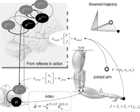
So what does free-energy bring to the table? If value is inversely pro-portional to surprise (see above), then free-energy is (an upper bound on) expected future cost. This makes sense, because optimal control theory assumes that action minimises expected cost, whereas the free-energy principle states that it minimises free-energy. Furthermore, the dynamical perspective provides a mechanistic insight into how policies are specified in the brain: Under the Principle of Optimality104 cost is the rate of change of value, which depends on changes in sensory states. This suggests that optimal policies can be prescribed by prior expectations about the motion of sensory states. Put simply, if priors induce a fixed-point attractor, when the states arrive at the fixed point, value will stop changing and cost will be minimised. A simple example is shown in Fig. 8, in which a cued arm movement is simulated using only prior expectations that the arm will be drawn to a fixed point (the target). This figure illustrates how computa-tional motor control110-114 can be formulated in terms of priors and the suppression of sensory prediction errors115. More generally, it shows how rewards and goals can be considered as prior expectations that action is obliged to fulfil24 (see also ref [116]).
However, fixed-point policies based on maximising value (mini-mising surprise) explicitly are flawed in two respects. First, they lead to fixed-point attractors, which are not viable solutions for agents immersed in environments with autonomous and dissipative dynamics. The second and slightly more subtle problem with optimal control and its ethological variants is that they assume the existence of a policy (flow though state-space) that always increases value. Mathematically, this assumes value is ‘Lyapunov function’ of the policy. Unfortunately, these policies do not necessarily exist. Technically, value is proportional to (log) eigensolution to the Fokker-Planck equation describing the density dynamics of an infi-nite number of agents pursuing the same policy under random fluctua-tions. This eigensolution is the equilibrium density and is a function of the policy. However, this does not imply that the policy or flow always increases value: According to the Helmholtz decomposition (also known as the fundamental lemma of vector calculus) flow can always be decom-posed into two components: an irrotational (curl-free) flow and a solenoi-dal (divergence-free) flow. When these components are orthogonal it is relatively easy to show that value is a Lyapunov function of the flow. However, there is no lemma or requirement for this orthogonality to exist and the Principle of Optimality104 is not guaranteed. In summary, although value can (in principle) be derived from the policy, the policy cannot (in general) be derived from the flow. So where does that leave us in a search for universal policies? We turn for an answer to itinerant poli-cies that are emerging as a new perspective on behaviour and purposeful self-organisation.
Fig. 8: A demonstration of cued-reaching movements. Lower right: motor plant, comprising a two-jointed arm with two hidden states, each of which corresponds to the angular position of joints. The position of the finger (black circle) is the sum of the vectors describing the loca -tion of each joint. Here, causal states in the world are the posi-tion and brightness of the tar -get (grey sphere). The arm obeys Newtonian mechanics, specified in terms of angular inertia and friction. Left: The brain senses hidden states directly in terms of proprioceptive input (sprop) that signals the angular positions (x1,x2) of the joints and indirectly, through seeing the location of the finger in space (j1,j2). In addition, the agent senses the target location (ν1,ν2) and brightness (ν3) through visual input (svisual). Sensory prediction errors are passed to higher brain levels to optimise the conditional expectations of hidden states (i.e., the angular position of the joints) and causal (i.e., target) states. The ensuing predictions are sent back to suppress sensory prediction errors. At the same time, sensory prediction errors are also trying to suppress themselves by changing sensory input through action. The grey and black lines denote reciprocal message-passing among neuronal populations that encode prediction error and conditional expectations; this architecture is the same as that depicted in Fig. 3. The descending black line represents motor control signals (predictions) from sensory state-units. The agent’s generative model includes priors on the motion of hidden states that effectively engage an invisible spring between the finger and target (when the target is illuminated). This induces a prior expectation that the finger will be drawn to the target, when cued appropriately. Insert (upper right): The ensuing movement trajectory caused by action. The black circles indicate the initial and final positions of the finger, which reaches the target (grey ball) quickly and smoothly.