THE DEVELOPMENT OF A SEMI-QUANTITATIVE DECISION SUPPORT SYSTEM FOR THE ESTIMATION OF MICROBIAL LOADING IN THE NEUSE WATERSHED
USING GEOGRAPHIC INFORMATION SYSTEMS
Anna Marlene Cressman
A thesis submitted to the faculty of the University of North Carolina at Chapel Hill in partial fulfillment of the requirements for the degree of Master of Science in the Department of
Environmental Sciences and Engineering of the School of Public Health.
Chapel Hill 2006
ABSTRACT
ANNA MARLENE CRESSMAN: The Development of a Semi-Quantitative Decision Support System for the Estimation of Microbial Loading in the Neuse Watershed Using
Geographic Information Systems
(Under the direction of Dr. Douglas Crawford-Brown)
Decision support systems (DSS) are often employed in complex environmental problems to provide the user with an integrated solution approach and can range from purely qualitative to quantitative modeling to fully automated. This paper presents a
semi-quantitative DSS approach for the problem of microbial loading in surface waters due to stormwater runoff. Six important stormwater variables are identified within the Neuse River Basin, N.C. Linear regression is used to assess the correlation of each variable with
TABLE OF CONTENTS
Page
LIST OF TABLES………v
LIST OF FIGURES……….vii
Chapter I A REVIEW OF THE LITERATURE………1
Introduction………1
Waterborne Disease Outbreaks Associated with Precipitation Events………...3
Microbial Exposure and Disease………...4
Factors that Influence the Rate of Runoff………….………...6
Stormwater Management……….………...8
Watershed Based Decision Support Systems………..10
II VARIABLE ANALYSIS……….……...13
Stormwater Variables………...13
Study Area………...13
Fecal Coliform………...15
Swine Density………...17
Soil Permeability………...20
Slope………...24
TABLE OF CONTENTS
Page Chapter
II
Precipitation…...………...33
Stream Flow………...37
III MICROBIAL LOADING DECISION SUPPORT SYSTEM…………...40
Semi-Quantitative Decision Support System………...40
Conclusion………...48
LIST OF TABLES
Table Page
2.1: Neuse Subbasin Areas……….... 15
2.2: Swine density by subbasin………... 18
2.3: Soil permeability by subbasin………...21
2.4: Soil permeability variables and associated r values……….... 24
2.5: Area and percent area with a slope greater than or equal to 10% by subbasin... 25
2.6: R-values for slope analysis with mean and max fecal coliform ... 28
2.7: Land use/Land cover categories……….. 29
2.8: Highly developed area and percent area by subbasin………...……….. 30
2.9: R-values associated with highly developed land use variables…………...……..… 33
2.10: Monthly mean and maximum precipitation and fecal coliform values for 2002-2005………...….……….. 35
2.11: Average stream flow velocity by subbasin………..37
3.1: Variable ranking according to predictive values derived from calculated r-values...41
3.2: Land area with low soil permeability rates...……….. 42
3.3: Percent of land with low soil permeability………. 42
3.4: Highly developed land areas... 43
3.5: Percent of land area that is highly developed………..43
3.6: Monthly precipitation………...………...43
LIST OF TABLES
Table Page 3.8: Land area with a slope greater than or equal to 10%…...………...44 3.9: Percent land area with a slope greater than or
LIST OF FIGURES
Figure Page
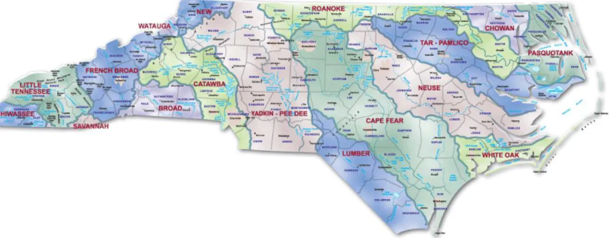
2.1: North Carolina river basins………...14
2.2: Neuse subbasins………...15
2.3: STORET stations………...16
2.4: Locations of swine operations in the Neuse………...…...17
2.5: Linear Regression Relation of Mean Fecal Coliform on Swine Density………...…...19
2.6: Linear Regression Relation of Maximum Fecal Coliform on Swine Density…...…...19
2.7: Soil permeability in the Neuse Basin………...21
2.8: Linear Regression Relation of Mean Fecal Coliform on Area of Soil with Less than or Equal to 2in/hr Permeability………....22
2.9: Linear Regression Relation of Maximum Fecal Coliform on Area of Soil with Less than or Equal to 2in/hr Permeability………....22
2.10: Linear Regression Relation of Mean Fecal Coliform on Percent of Land Area with Less than or Equal to 2in/hr Permeability………...23
2.11 Linear Regression Relation of Maximum Fecal Coliform on Percent of Land Area with Less than or Equal to 2in/hr Permeability………...23
2.12: Areas within the Neuse basin with a slope of greater than or equal to 10%………...25
2.13: Linear Regression Relation of Mean Fecal Coliform on Area with a Slope Greater than or Equal to 10% Rise...………...26
2.14: Linear Regression Relation of Maximum Fecal Coliform on Area with a Slope Greater than or Equal to 10% Rise….………...26
LIST OF FIGURES
Figure Page 2.17: Highly developed areas………...……....30 2.18: Linear Regression Relation of Mean Fecal Coliform on
Highly Developed Land Area………..31 2.19: Linear Regression Relation of Maximum Fecal Coliform on
Highly Developed Land Area………..31 2.20: Linear Regression Relation of Mean Fecal Coliform on Percent
Highly Developed Land Area………..32 2.21: Linear Regression Relation of Maximum Fecal Coliform on Percent
Highly Developed Land Area………..32 2.22: Average annual precipitation in the Neuse basin…...………....34 2.23: Location of precipitation monitoring stations in the Neuse basin... 35 2.24: Linear Regression Relation of Monthly Mean Fecal Coliform on
Monthly Mean Precipitation……...….36 2.25: Linear Regression Relation of Monthly Maximum Fecal Coliform on
Monthly Maximum Precipitation……...….36 2.26: Locations of USGS stream monitoring stations………...37 2.27: Linear Regression Relation of Mean Fecal Coliform on
Mean Stream Flow Velocity………38 2.28: Linear Regression Relation of Maximum Fecal Coliform on
Chapter I:
A REVIEW OF THE LITERATURE
Introduction
Recently, the association between waterborne disease outbreaks and precipitation patterns has been analyzed as concern over how population growth, land use, and climate change may affect the incidence of infectious diseases. A waterborne disease outbreak is defined as an event in which two or more persons experience similar illnesses after ingestion or contact with drinking or recreational/occupational water sources and for which
epidemiological evidence confirms water as the most likely source of illness (Lee et al. 2002). A study completed by Curriero et al. found precipitation had an integral role in the occurrence of waterborne disease outbreaks in the U.S. between 1948 and 1994. Of the 548 outbreaks reported during this period, 51% were found to have occurred within two months of an extreme precipitation event, defined as a rainfall event falling within the highest 10% of precipitation for the given watershed in the 2-month period leading up to the outbreak
Stormwater runoff refers to excess rainwater that is not absorbed by the ground (Davies and Bavor 2000). It is generated during precipitation events and may deliver potentially harmful pollutants to receiving waters. In addition to precipitation, other variables such as soil type, impervious surface area and slope play a role in runoff generation. Pathogens from this stormwater runoff reach surface waters and have
contributed to the contamination of an estimated 5529 water bodies across the U.S., making pathogens the second highest cause of water impairment next to sediment (Gaffield et al. 2003). In urban areas, 60% of the annual load of contaminants is transported during a storm event (Curriero et al. 2001). Stormwater runoff contains a variety of contaminants including microbes, chemicals, and sediments. Bacterial pathogens such as Shigella spp. and
Salmonella spp.; protozoa such as Cryptosporidium parvum and Giardia spp.; and viral agents such as Norwalk-like virus are commonly found in stormwater runoff. Fecal coliform levels are the most widely used indicator for pathogenic contamination of waters. The Center for Watershed Protection has estimated that stormwater runoff contains a mean fecal coliform concentration of about 15,000 CFU per 100mL (CWP 1999). Fecal coliform levels have been positively correlated with precipitation intensity and negatively correlated with salinity levels of brackish receiving water, Lake Pontchartrain in Louisiana, indicating the water is inundated with contaminated freshwater runoff after a storm event (Barbé et al. 2001). This study also found that precipitation events effect fecal coliform concentrations up to 2-3 days after the event occurs. The time period studied was characterized by lower than average rainfall, indicating a more severe relationship between fecal coliform
Waterborne Disease Outbreaks Associated with Precipitation Events
Waterborne disease outbreaks require four main elements: a source of contamination or pathogens, fate and transport of that contamination to a water supply, failure to properly treat the contamination, and detection or reporting of the illnesses (Curriero et al. 2001). Precipitation events aid in transporting the pathogen source to the water supply. Once a water supply is contaminated, humans may become exposed to the microbes through drinking water, incidental ingestion while recreationally coming in contract with the water, dermal absorption, or inhalation of aerosolized microbes.
Several waterborne disease outbreaks have occurred recently that demonstrate the connection between stormwater runoff and associated variables such as precipitation, slope, and land cover. The most notable outbreak occurred in Milwaukee, W.I. in the spring of 1993 when over 400,000 people became ill after ingestion of drinking water contaminated with Cryptosporidium parvum, and 58 people eventually died from the associated illness (Hoxie et al. 1997). Although the exact source of contamination for this outbreak is still speculated upon, the most likely sources include cattle manure, slaughterhouses, or human sewage that was transported through the rivers leading to Lake Michigan after spring rains and snowmelt runoff (MacKenzie et al. 1995). Drinking water drawn from the lake was then inadequately treated before distribution to homes. Once it enters into surface waters,
Bacterial contamination was responsible for the outbreak of E.coli 0157:H7 and
Campylobacter jejuni in Walkerton, Ontario in May 2000 where 2,300 people became ill and 7 died (Hrudley et al. 2003). This outbreak was caused by contamination of a shallow well by cattle manure after heavy spring rainfall. Because bacteria such as E. coli and
Campylobacter can be effectively removed through disinfection, inadequate chlorine disinfection in the Walkerton distribution system played a major role in this outbreak.
Hrudley also discusses several other outbreak events that have been linked directly to heavy rainfall or snowmelt in both North American and Europe. Campylobacter,Giardia, and Cryptosporidium were the main pathogens associated with these events. An outbreak of
Cryptosporidium in New Jersey in 1994 lasted 4 weeks and infected over 2,000 people. The source of this outbreak was most likely failing septic systems. Pathogens released by these systems were carried to a shallow lake through stormwater runoff following a rain event (Kramer et al. 1998).
Microbial Exposure and Disease
In the EPA’s Guidelines for Exposure Assessment, intake of an external agent occurs when the agent crosses over the outer layer of the human body, through openings in the mouth or nose or through dermal absorption (EPA 1992). Humans can become exposed to viral, bacterial, and protozoan pathogens through ingestion of contaminated drinking water or incidental ingestion while swimming. Dermal contact with polluted waters and inhalation of aerosolized microbes are two other potential routes of exposure.
host body. Symptoms of these microbial induced diseases include fever, abdominal pain, diarrhea, and vomiting (EPA 1993). Often gastrointestinal illnesses are underreported, due to the relatively low mortality rate associated with them. The very young or old and immuno-compromised individuals are usually the populations at risk for serious outcomes of
gastroenteritis. In the massive cryptosporidiosisoutbreak that occurred in Milwaukee in 1993, officials were not alerted to the existence of the outbreak until reports of widespread school and work absenteeism and shortages of antidiarrhoeal medication reached the city health department (Proctor et al. 1998).
Microbial contamination can be derived from a variety of sources within a watershed, largely depending upon the population and land use patterns of the area. The most common sources of microbes include combined sewer overflows (CSO’s), sanitary sewer overflows (SSO’s), illegal sanitary connections to storm drains, direct discharge of wastewater into water bodies or storm drains, failing septic systems, and domestic and wild animal fecal contamination (NCNERR 2004, Davies and Bavor 2000). North Carolina is the second biggest hog farming state, and many watersheds with large hog populations experience high amounts of microbial contamination from the wastes they produce (Osterberg and Wallinga 2004).
Both total and fecal coliform levels are often measured to determine water quality through either a most probable procedure method or a membrane filtration process (Madigan et al. 2003). In general, when fecal coliform levels are measured above 105CFU/ 100mL, human fecal contamination is the most likely explanation (CWP 1999). Other indicators of water quality include E.coli,Clostridum perfringens, and enterococci. These indicators are often more accurate than coliform levels, but correlating their concentrations to concentrations of pathogens is still being studied (Griffin et al. 2001).
Factors that Influence the Rate of Runoff
Many factors influence the rate at which stormwater runoff reaches receiving waters. Land use, extent of impervious surfaces, and the degree of connection between pathogen sources and receiving waters as well as hydrological factors such as slope, soil type, and precipitation patterns are important considerations (Tsihrintzis and Hamid 1997).
Construction projects also pose a concern and may accelerate soil erosion by up to 40,000 times the previous rate. Eroding sediment can carry a significant amount of pathogens to receiving waters (Gaffield et al. 2003). Initial exceedance of sewer capacities due to
increased infiltration and clogging of the systems may lead to the generation of contaminated stormwater in areas with both sanitary and combined sewer systems (Field and O’Connor 1997).
temperature leads to a 6% increase in atmospheric holding of water vapor (Epstein 1999). In a study of precipitation trends in the U.S. in since 1910, Karl and Knight found in increase in both the number of days per year with precipitation and the intensity of the precipitation events, with the most pronounced changes occurring in the spring and autumn (1997).
Climatic models have also suggested an increase in summer droughts for
mid-continental areas (Meehl et al. 2000). Extreme precipitation events following such a drought period may lead to high rates of runoff due to the inability of the dry soil to effectively absorb the rainfall (Tsihrintzis and Hamid 1997). In an analysis of stormwater runoff in the Minneapolis-St. Paul, MN area, Brezonik and Stadelmann found the most important variables of their multi-linear regression models to predict runoff volume included precipitation amount, drainage area and percent impervious surface (2002). Mallin et al. found fecal coliform levels to be most influenced by the percent of impervious surfaces in a watershed, accounting for 95% of the variability in fecal coliform levels in a given estuary (2000a).
watersheds containing animal operations (Mallin et al. 2001). Graczyk et al. specifically identified watersheds containing cattle operations located within 100-year floodplain areas as especially likely sources of Cryptosporidium to receiving waters (2000).
In the Neuse River Basin, an estimated 441 point discharges release 3.34 x 10⁸L of effluent per day. Also, the watershed contains over 550 confined animal feeding operations (CAFO’s) of which 76% are hog farms and 23% are poultry operations (Glasgow and Burkholder 2000). These CAFO’s also contribute a significant amount of effluent to the watershed. There have been several instances of waste lagoon rupture, due to heavy
precipitation and hurricane events, sending millions of gallons of fecal matter into the basin (Mallin 2000b). It is estimated that the average 135 lb. hog produces about 11 lbs. of manure each day and 1.9 tons of manure annually (NCSU 2006).
Stormwater Management
Stormwater management strategies include best management practices (BMP’s) that are designed to eliminate pollutant loading into stormwater runoff and nearby receiving waters. A comprehensive review of many BMP’s to reduce the impact of stormwater runoff has been compiled by the Urban Water Resources Research Council of the American Society of Engineers. The National Stormwater Best Management Practices Database includes structural BMP’s such as detention, retention, infiltration and wetland basins and
development and incorporation of buildings with green roofs are examples of BMP’s that can be utilized to minimize the negative impacts of stormwater runoff (Gaffield et al. 2003).
Constructed wetlands are shallow detention systems that are highly vegetated and reduce pathogen concentrations through physical, chemical and biological processes (Davies and Bavor 2000). They can reduce the amount of particles reaching receiving waters from stormwater runoff, but the exact removal time depends on the species measured and has varied across studies. Stenström and Carlander found E.coli and fecal enterococci to have 90% die off rates at 26 and 40 days on average, respectively. More environmentally resistant strains, such as Clostridium perfringens, may last an average of 324 days before 90%
reduction (2001). The effectiveness of constructed wetlands at treating swine wastewater has been measured at 96, 97, and 99% reductions in Salmonella, fecal coliform and E.coli,
respectively. Virus indicators, somatic and F-specific coliphages, were also reduce by 99 and 98%, respectively (Hill and Sobsey 2001). Davies and Bavor found the survival rates of both
E.coli and Salmonella to be correlated with particle size, with both species surviving longer in sediments containing at least 25% clay (2000). The construction of upstream rainwater storage tanks may also reduce the volume of run-off during storm events. The effectiveness of such tanks depends largely on their storage capacities relative to potential infiltration volumes and modeling using continuous peak rainfall simulations should be used to determine the maximum storage needed under extreme conditions (Vaes and Berlamont 2002).
Griesel 2003). GIS analysis can be implemented to take into consideration a watershed’s specific parameters, such as topography, soil, and hydrology to predict the impacts of stormwater runoff (Thornhill 1994).
Watershed Based Decision Support Systems
Decision support systems (DSS) aid people in making decisions by integrating information from a variety of sources (Fulcher et al. 2006). They help decision makers to identify the problem, involve stakeholders, and implement integrated solutions. Generally, a DSS is employed when a particular problem is posed to decision makers, such as the
potential for microbial contamination of surface waters due to stormwater runoff. A DSS may range in complexity from purely qualitative- the decision maker is guided through a series of subjective questions, to quantitative- the DSS is based upon mathematical relationships and modeling of the variables, to completely automated- the user supplies variable data and the DSS performs all necessary calculations to produce a solution. The DSS specifies the attributes or variables that should be considered given the particular problem and assigns them a value, given their relative importance based on either subjective
judgments or mathematical computations. Each of the attributes within the scaling are then assigned a weight, given their unique range of values. The most extensive DSS then provide an algorithm for combining all of the variables, their assigned scales and values to simulate potential decision outcomes.
watershed decisions (Fulcher et al. 2006). These systems often involve complex modeling and require detailed, resource intensive data sets. Hydrologic models housed within the systems may involve a large degree of uncertainty. Uncertainty involving parameters, processes, data, and initial conditions all contribute to the overall uncertainty of a model output (Zehe et al. 2005). Fulcher et al. has detailed a Watershed Management Decision Support System (WAMADSS) that involves the integration of a GIS, an economic model, and two environmental simulation models (2006). This DSS, like many others, allows for the consideration of both economic and environmental variables in watershed management but requires the expenditure of a large amount of resources to accurately populate the models.
Given the large amount of data already available on variables associated with stormwater runoff, there exists a need for a DSS that incorporates this data into an easily understandable framework that does not require extensive resource expenditure. The
accuracy of the final DSS output will not be as high as the more model intensive DSS options already created, but this DSS would present a reasonable first estimate of watershed
Chapter II
VARIABLE ANALYSIS
Stormwater Variables
Six variables were selected in this study to be regressed against fecal coliform levels in the Neuse to establish a scale of their importance in determining the risk for fecal coliform contamination. These variables were chosen after a review of the literature and past studies suggested their correlations with fecal contamination in other basins and include: swine density, soil permeability, slope, highly developed land area, precipitation, and average stream flow velocity. For each variable, a GIS data layer was created using ESRI’s ArcGIS 9.1. The variables were selected by the 14 subbasins and a new layer was created for each variable in each subbasin. The values for these variables on a subbasin level were then used in a linear regression to determine the correlation between the variable and the fecal coliform values observed in the subbasins.
Study Area
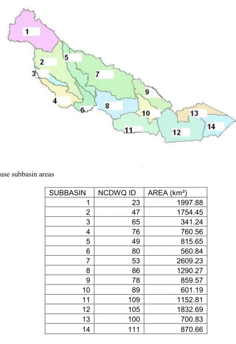
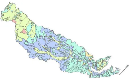
Nineteen North Carolina counties have 2% or greater of their area located within the Neuse and include Beaufort, Carteret, Craven, Duplin, Durham, Franklin, Granville, Greene, Johnson, Jones, Lenoir, Nash, Orange, Pamlico, Person, Pitt, Wake, Wayne, and Wilson counties. According to the 2000 US Census, the Neuse Basin has a population of 1,353,617 persons and a population density of 211 persons/ sq.mi. This density is slightly higher than the North Carolina average of 139 persons/ sq. mi. and is expected to increase throughout the basin, especially in the upper basin areas of Wake and Durham counties. The swine industry dominates the basin’s animal operations, with 460 registered swine operations as of 2002 housing almost 2 million swine. Around 3,500 miles of freshwater streams are located within the basin. The basin also includes 19 fresh water reservoirs, including 14 lakes which are designated as drinking water supplies (NCDENR 2002). The following map displays the Neuse Basin and the subbasin numbers used in this study (Fig. 2.2). The table below gives the areas (including land and water) of the subbasins in square kilometers (Table 2.1).
SUBBASIN NCDWQ ID AREA (km²)
1 23 1997.88
2 47 1754.45
3 65 341.24
4 76 760.56
5 49 815.65
6 80 560.84
7 53 2609.23
8 86 1290.27
9 78 859.57
10 89 601.19
11 109 1152.81
12 105 1832.69
13 100 700.83
14 111 870.66
Fecal Coliform
Fecal coliform is one common indicator of water quality impairment by pathogenic organisms. Other indicators include E. coli,Clostridium perfringens, and coliphages.
Fig. 2.2: Neuse subbasins (USDA-NCRS 1998b)
relative ease of detection as compared to pathogenic organisms. Indicator organisms are often not pathogenic themselves but occur with pathogenic organisms and are a sign of fecal contamination (NPS 2005). Fecal coliform presence correlates most strongly to bacterial pathogens and is used in this study due to the abundance and thoroughness of available data.
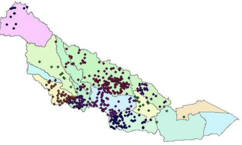
Fecal coliform data was attained from the Environmental Protection Agency’s (EPA) STORET database by searching for results by geographic area and entering in the Neuse basin counties. The STORET database provides water quality data collected by both state and federal agencies. All data is housed in this centralized repository for easy access and retrieval. Data used in this study was originally collected by the North Carolina Division of Water Quality and was available for the Neuse Basin from 1994-2005 (EPA 2006). Fecal coliform data was available for individual stations throughout the basin and identified by station number and latitude and longitude coordinates. ESRI’s ArcGIS 9.1 was used to plot and project this information onto a GIS of the Neuse basin and its subbasins. The map below displays station locations throughout the basin (Fig. 2.3).
There are a total of 184 stations in the Neuse basin. Subbasin 2 had the highest average fecal coliform value at 516.04 cfu/100mL, while subbasin 14 had the lowest at 3.36 cfu/100mL. Subbasin 1 had the highest overall peak with 30,000 cfu/100mL measured in 1996. There was no data available for subbasins 4 and 6 due to the lack of monitoring stations in these subbasins. Therefore, only 12 subbasins were used to determine the relationships between stormwater variables and fecal coliform levels. To determine the subbasin assigned to each station, ArcGIS’s “Select by Location” tool was applied. The data points with their centers in each subbasin were selected and exported into a new data layer.
Swine Density
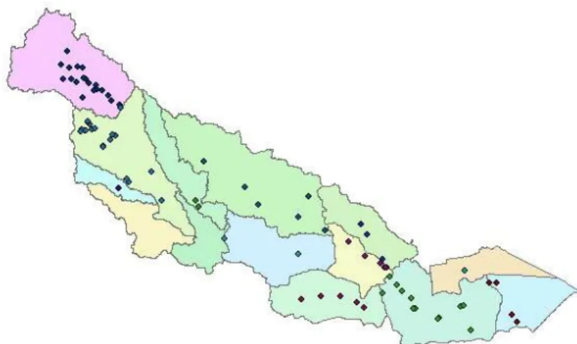
The swine population data used in this study was collected in 2002 by the North Carolina Department of Environment and Natural Resources, Division of Water Quality, and reflects the number of swine located in the animal operations in the Neuse. The map below shows the locations of swine operations throughout the Neuse (Fig. 2.4).
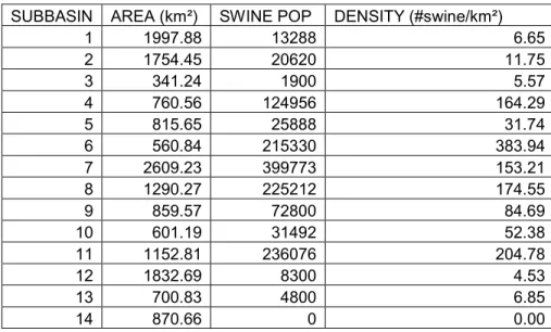
Swine density was calculated by dividing the total swine population in a subbasin by the area in km². The resulting values are shown in the table below (Table 2.2).
SUBBASIN AREA (km²) SWINE POP DENSITY (#swine/km²)
1 1997.88 13288 6.65
2 1754.45 20620 11.75
3 341.24 1900 5.57
4 760.56 124956 164.29
5 815.65 25888 31.74
6 560.84 215330 383.94
7 2609.23 399773 153.21
8 1290.27 225212 174.55
9 859.57 72800 84.69
10 601.19 31492 52.38
11 1152.81 236076 204.78
12 1832.69 8300 4.53
13 700.83 4800 6.85
14 870.66 0 0.00
Subbasin 6 had the highest swine density with 383.94 swine/km² while subbasin 12 had the lowest density at 4.53 swine/km² and subbasin 14 had a density of zero due to the lack of swine operations in that subbasin. Given the lack of fecal coliform data in subbasins 4 and 6 and the swine density of zero in subbasin 14, only 11 subbasins were used in the swine density regression analysis to determine the strength of the relationship between swine density and fecal coliform levels. The lack of fecal coliform data in subbasin 6, the subbasin with the highest swine density may have had an effect on the observed relationships. Swine density was regressed against both mean and maximum fecal coliform concentrations in the 11 subbasins using Microsoft Excel. The resultant graphs are displayed below (Fig. 2.5 and Fig 2.6).
Linear Regression Relation of Mean Fecal Coliform on Swine Density
y = -0.743x + 270.94 R2= 0.1581
0 100 200 300 400 500 600
0.00 50.00 100.00 150.00 200.00 250.00
Swine Density (#/sq.km.)
F ec al C o li fo rm (c fu /1 0 0 m l)
Linear Regression Relation of Maximum Fecal Coliform on Swine Density
y = -81.335x + 15997 R2= 0.3061
0 5000 10000 15000 20000 25000 30000 35000
0.00 20.00 40.00 60.00 80.00 100.00 120.00 140.00 160.00 180.00 200.00
Swine Density (#/sq.km.)
F ec al C o li fo rm (c fu /1 0 0 m l)
The regression lines generated from the data indicate swine density is a somewhat important predictor of fecal coliform contamination within the subbasins of the Neuse. The r-values of r = 0.39 for mean fecal coliform and r = 0.55 for maximum fecal coliform suggest a medium
Fig. 2.5
to weak correlation. The negative slope of the regression lines indicate that swine density within a subbasin may not necessarily correlate to impairment in that subbasin. The trend lines on the above graphs indicate that either larger swine operations do a better job of containing their waste or waste from the larger operations is being runoff into other subbasins.
Soil Permeability
Soil permeability, or the rate at which water flows through the porous medium of soil, plays an important role in the amount of water that can be absorbed and subsequently the amount of water that is runoff during a given storm event. Soil data for the Neuse basin was obtained from the National Resources Conservation Service (NCRS) at the U.S. Department of Agriculture as part of the State Soil Geographic (STATSGO) database collected in 1994 (USDA-NCRS 1994). Permeability is one of the characteristics available from the
Table 2.3 below displays the values calculated for soil permeability in each subbasin.
SUBBASIN TOTAL AREA (km²) AREA (km²) /2 in/hr PERCENT (%) /2 in/hr
1 1997.88 1863.37 93.27
2 1754.45 928.68 52.93
3 341.24 151.24 44.32
5 815.65 375.81 46.07
7 2609.23 96.97 3.72
8 1290.27 202.35 15.68
9 859.57 149.43 17.38
10 601.19 18.08 3.01
11 1152.81 7.46 0.65
12 1832.69 346.15 18.89
13 700.83 208.75 29.79
14 870.66 42.01 4.82
Subbasin 1 has both the largest area and percent of area within the basin with permeability Q
2in/hr while subbasin 11 has the smallest area and percent area covered by low permeability soils. Both area and percent area were then regressed against mean and maximum fecal
Fig. 2.7: Soil permeability in the Neuse Basin (USDA-NCRS 1994).
coliform levels using Microsoft Excel. The resultant graphs are displayed below (Fig. 2.8 -Fig. 2.11).
Linear Regression Relation of Mean Fecal Coliform on Area of Soils with Less than or Equal to 2in/hr Permeability
y = 0.2118x + 104.54 R2= 0.5402
0 100 200 300 400 500 600
0.00 200.00 400.00 600.00 800.00 1000.00 1200.00 1400.00 1600.00 1800.00 2000.00
Area (km^2) F e ca l C o li fo rm (c fu /1 00 m L )
Linear Regression Relation of Maximum Fecal Coliform on Area of Soils with Less than or Equal to 2in/hr Permeability
y = 16.522x + 984.44 R2= 0.9367
0 5000 10000 15000 20000 25000 30000 35000
0.00 200.00 400.00 600.00 800.00 1000.00 1200.00 1400.00 1600.00 1800.00 2000.00
Linear Regression Relation of Mean Fecal Coliform on Percent of Land Area with Less than or Equal to 2in/hr Permeability
y = 4.1162x + 68.645 R2= 0.5424
0 100 200 300 400 500 600
0.00 10.00 20.00 30.00 40.00 50.00 60.00 70.00 80.00 90.00 100.00
Percent Land Area w/in a Subbasin (%)
F e ca l C o li fo rm (c fu /1 00 m L )
Linear Regression Relation of Maximum Fecal Coliform on Percent of Land Area with Less than or Equal to 2in/hr Permeability
y = 279.99x - 682.96 R2= 0.7151
-5000 0 5000 10000 15000 20000 25000 30000 35000
0.00 10.00 20.00 30.00 40.00 50.00 60.00 70.00 80.00 90.00 100.00
Percent Land Area w/in a Subbasin (%))
F e c al C o li fo rm (c fu /1 0 0m L )
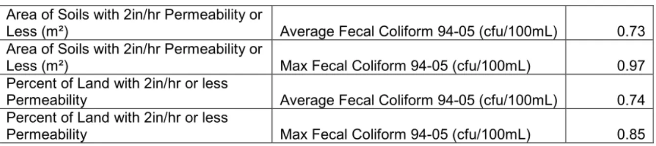
The regression analysis for both land area in km² and percent land area indicates soil permeability is an important indicator of potential fecal contamination in the Neuse basin.
Fig. 2.10
Area of Soils with 2in/hr Permeability or
Less (m²) Average Fecal Coliform 94-05 (cfu/100mL) 0.73
Area of Soils with 2in/hr Permeability or
Less (m²) Max Fecal Coliform 94-05 (cfu/100mL) 0.97
Percent of Land with 2in/hr or less
Permeability Average Fecal Coliform 94-05 (cfu/100mL) 0.74
Percent of Land with 2in/hr or less
Permeability Max Fecal Coliform 94-05 (cfu/100mL) 0.85
The high r-values observed in this regression analysis, especially with respect to maximum fecal coliform concentrations, indicate a strong correlation between low soil permeability and fecal coliform levels. These relationships suggests that areas within the Neuse with low permeability are more susceptible to fecal contaminated runoff to surface waters than areas with higher permeability.
Slope
A digital elevation model (DEM) of the Neuse basin was obtained from the U.S. Geological Survey (USGS) National Elevation Dataset and has a resolution of 30 meters (USGS 2004). To calculate slope from this dataset, the “slope” tool within ArcGIS’s spatial analyst toolset was used. ArcGIS uses the DEM to calculate slope by estimating the
elevation at a given point and comparing the elevation of that point to the elevations of surrounding points, which have all been given a weight (Longley et al. 2005). In this study, slope was measured in percent rise and “high slope” was defined as a slope greater than or equal to 10%. According to a Development Ordinance from the Town of Chapel Hill, located in subbasin 1, development on land with a 10% slope or greater requires special site preparations and design techniques (TCH 2000). Areas with a slope of 25% or greater are generally considered unsuitable for development (MacDonald and Holmes 2004). Areas of
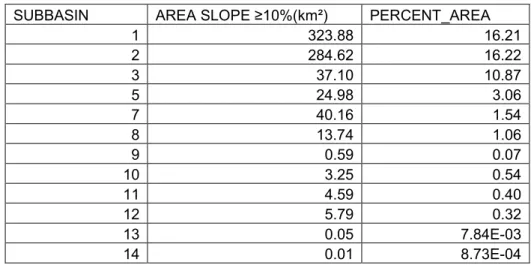
areas within the subbasins that have a slope of greater than or equal to a 10% rise. The calculated values are displayed in Table 2.5 below.
SUBBASIN AREA SLOPE @10%(km²) PERCENT_AREA
1 323.88 16.21
2 284.62 16.22
3 37.10 10.87
5 24.98 3.06
7 40.16 1.54
8 13.74 1.06
9 0.59 0.07
10 3.25 0.54
11 4.59 0.40
12 5.79 0.32
13 0.05 7.84E-03
14 0.01 8.73E-04
Subbasins 1 and 2 had the largest area of high slope by far while the most coastal of the subbasins, 14, had the smallest area of high slope. Slope values for subbasins 4 and 6 were omitted due to the lack of fecal coliform data in these subbasins. The values for area and percent area of high slope were regressed against fecal coliform data to generate the flowing graphs using Microsoft Excel (Fig. 2.13 and Fig. 2.14).
Fig. 2.12: Areas within the Neuse basin with a slope of greater than or equal to 10%.
Linear Regression Relation of Mean Fecal Coliform on Area with a Slope Greater than or Equal to 10 % Rise
y = 1.1581x + 110.72
R2= 0.7445
0 100 200 300 400 500 600
0.00 50.00 100.00 150.00 200.00 250.00 300.00 350.00
Area with a Slope Greater than or Equal to 10% (km^2)
F ec al C o lif o rm (c fu /1 00 m L )
Linear Regression Relation of Maximum Fecal Coliform on Area with a Slope Greater than or Equal to 10 % Rise
y = 76.972x + 2290.5
R2= 0.937
0 5000 10000 15000 20000 25000 30000 35000
0.00 50.00 100.00 150.00 200.00 250.00 300.00 350.00
Area with a Slope Greater than or Equal to 10 % (km^2)
Linear Regression Relation of Mean Fecal Coliform on Percent Area of Slope Greater than or Equal to 10 % Rise
y = 20.963x + 94.144
R2= 0.7552
0 100 200 300 400 500 600
0.00 2.00 4.00 6.00 8.00 10.00 12.00 14.00 16.00 18.00
Percent Area with Slope Greater than or Equal to 10% (%)
F ec al C o li fo rm (c fu /1 00 m L )
Linear Regression Relation of Maximum Fecal Coliform on Percent Area of Slope Greater than or Equal to 10% Rise
y = 1231x + 1868.7
R2= 0.742
0 5000 10000 15000 20000 25000 30000 35000
0.00 2.00 4.00 6.00 8.00 10.00 12.00 14.00 16.00 18.00
Percent Area with Slope Greater than or Equal to 10% (%)
F ec al C o li fo rm (c fu /1 00 m L )
The regression analysis of slope against both mean and maximum fecal coliform levels in the
Fig. 2.15
waters and is an important predictive variable when considering area of high slope and percent area of high slope within a subbasin. The following table displays the r-values generated (Table 2.6).
Area of High Slope (@10%) Average Fecal Coliform 94-05 (cfu/100mL) 0.86
Area of High Slope (@10%) Max Fecal Coliform 94-05 (cfu/100mL) 0.97
Percent Area of High Slope (@10%) Average Fecal Coliform 94-05 (cfu/100mL) 0.87
Percent Area of High Slope (@10%) Max Fecal Coliform 94-05 (cfu/100mL) 0.86
The r-values for each correlation are all above 0.85 indicating a strong relationship between slope and this particular pollutant. According to this analysis, slope values in a given subbasin are an important predictor of potential surface water contamination.
Highly Developed Land Area
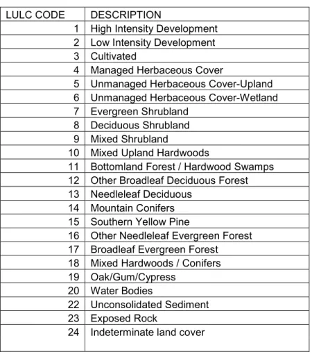
Highly developed land area generally includes less area for stormwater runoff to be contained or absorbed, resulting in increased rates of runoff. Highly developed land often includes a large amount of impervious surfaces, such as roads, parking lots and buildings. Land use/ land cover data used in this study was compiled by US Environmental Protection Agency, Region IV Wetlands Division; North Carolina Department of Transportation; North Carolina Center for Geographic Information and Analysis; numerous universities, colleges, municipalities and county governments and was obtained on the UNC campus network (EarthSat 1998). This data categorized land use/ land cover into 24 categories displayed in the table below (Table 2.7).
LULC CODE DESCRIPTION
1 High Intensity Development 2 Low Intensity Development 3 Cultivated
4 Managed Herbaceous Cover
5 Unmanaged Herbaceous Cover-Upland 6 Unmanaged Herbaceous Cover-Wetland 7 Evergreen Shrubland
8 Deciduous Shrubland 9 Mixed Shrubland
10 Mixed Upland Hardwoods
11 Bottomland Forest / Hardwood Swamps 12 Other Broadleaf Deciduous Forest 13 Needleleaf Deciduous
14 Mountain Conifers 15 Southern Yellow Pine
16 Other Needleleaf Evergreen Forest 17 Broadleaf Evergreen Forest 18 Mixed Hardwoods / Conifers 19 Oak/Gum/Cypress
20 Water Bodies
22 Unconsolidated Sediment 23 Exposed Rock
24 Indeterminate land cover
According to the NC Land Use Standard, high intensity land use includes:
“Areas of intensive use with much of the land covered by structures. Included in this category is land used for residential, commercial, and industrial purposes; colleges; strip developments along highways; transportation, power, and
communications facilities; areas developed for passive or active recreational
purposes; and such isolated units as mills, mines, and quarries, shopping centers, and institutions.” (NCCGIA 1994)
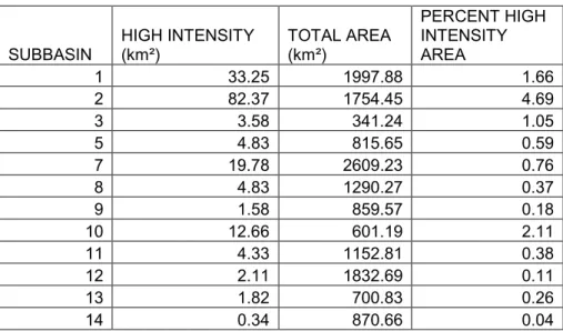
Areas within each subbasin categorized as “High Intensity” LULC were calculated and are displayed in purple on the following map (Fig. 2.17) and table (Table 2.8).
SUBBASIN HIGH INTENSITY (km²) TOTAL AREA (km²)
PERCENT HIGH INTENSITY AREA
1 33.25 1997.88 1.66
2 82.37 1754.45 4.69
3 3.58 341.24 1.05
5 4.83 815.65 0.59
7 19.78 2609.23 0.76
8 4.83 1290.27 0.37
9 1.58 859.57 0.18
10 12.66 601.19 2.11
11 4.33 1152.81 0.38
12 2.11 1832.69 0.11
13 1.82 700.83 0.26
14 0.34 870.66 0.04
Subbasins 1 and 2 have the largest amount of highly developed land area. These subbasins include the urban areas of Durham, Raleigh, and Cary. Subbasin 14 has the smallest amount of highly developed land area. Both highly developed land area and percent of highly developed land area were regressed against mean and maximum fecal coliform data using Microsoft Excel and the following graphs were produced (Fig. 2.18 – Fig. 2.21).
Fig. 2.17: Highly developed land areas.
Linear Regression Relation of Mean Fecal Coliform on Highly Developed Land Area
y = 5.3326x + 105.82 R2= 0.6651
0 100 200 300 400 500 600
0 10 20 30 40 50 60 70 80 90
Highly Developed Land Area (km^2)
F ec al C o li fo rm (c fu /1 0 0m L )
Linear Regression Relation of Maximum Fecal Coliform on Highly Developed Land Area
y = 286.62x + 2933.2 R2= 0.5474
0 5000 10000 15000 20000 25000 30000 35000
0 10 20 30 40 50 60 70 80 90
Highly Developed Land Area (km^2)
Linear Regression Relation of Mean Fecal Coliform on Percent Highly Developed Land Area
y = 86.605x + 93.871 R2= 0.5552
0 100 200 300 400 500 600
0 0.5 1 1.5 2 2.5 3 3.5 4 4.5 5
Percent Highly Developed Land (%)
F ec al C o li fo rm (c fu /1 0 0m L )
Linear Regression Relation of Maximum Fecal Coliform on Percent Highly Developed Land Area
y = 4308.2x + 2644.1
R2= 0.3915
0 5000 10000 15000 20000 25000 30000 35000
0 0.5 1 1.5 2 2.5 3 3.5 4 4.5 5
Percent Highly Developed Land (%)
All four regressions performed regarding fecal coliform and highly developed land indicate a strong correlation between these variables. The variables and their respective r-values are displayed in the table below (Table 2.9).
Highly Developed Land Area (m²)
Average Fecal Coliform 94-05
(cfu/100mL) 0.81 Highly Developed Land Area (m²) Max Fecal Coliform 94-05 (cfu/100mL) 0.74 Percent Highly Developed Land
Area
Average Fecal Coliform 94-05
(cfu/100mL) 0.75 Percent Highly Developed Land
Area Max Fecal Coliform 94-05 (cfu/100mL) 0.63
From these r-values, it is apparent that total highly developed land area within a subbasin correlates well with the mean and maximum values of fecal coliform in the surface waters. Percent highly developed land area also demonstrates a high correlation to fecal coliform levels, but the strength of the relationship is not as great as it is with the land area, especially when considering the correlation to maximum fecal coliform levels.
Precipitation
Average annual precipitation data (in/yr) was obtained from USDA/NRCS: National Cartography and Geospatial Center and covers the climatic period from 1961-1990 (Daly and Taylor 1998). Average precipitation throughout the Neuse was relatively uniform, with a range of 46-57 in/yr in the 14 subbasins (Fig. 2.22).
Due to the relative uniformity of annual precipitation averages across the basin, it was concluded that precipitation may exhibit more of a correlation with fecal coliform when considered temporally throughout the basin, rather than spatially varying from subbasin to subbasin. Monthly precipitation averages and maximums were obtained from the State Climate Office of North Carolina (NCSU) for the period of 2002-2005. The map below displays the location of precipitation monitoring stations (Fig. 2.23) and the following table displays the values used in this analysis (Table 2.10).
Mean Precip 02-05
(in) Mean FC 02-05 (cfu/100mL) Max Precip 02-05 (in) Max FC 02-05 (cfu/100mL)
JAN 1.83 220.52 4.07 3,500.00
FEB 3.40 141.37 9.26 3,900.00
MAR 3.61 207.58 7.98 9,700.00
APR 3.54 251.77 8.17 4,500.00
MAY 4.27 247.60 11.27 5,000.00
JUN 4.05 136.28 9.74 2,000.00
JUL 5.48 198.46 13.67 6,200.00
AUG 5.82 921.75 16.84 21,000.00
SEP 4.18 380.31 11.52 11,000.00
OCT 4.54 228.90 14.64 6,900.00
NOV 3.06 205.37 6.23 3,400.00
DEC 3.50 104.29 7.72 2,000.00
The monthly precipitation data was used in a linear regression with mean and maximum fecal coliform values. Fecal coliform data in the analysis of this variable was limited to 2002-2005 due to the temporal nature of precipitation. The following two graphs were generated using Microsoft Excel (Fig. 2.24 and 2.25)
Fig. 2.23: Location of precipitation monitoring stations in the Neuse basin (NCSU 2006).
Linear Regression Relation of Monthly Mean Fecal Coliform on Monthly Mean Precipitation
y = 114.63x - 181.25
R2= 0.3154
0.00 100.00 200.00 300.00 400.00 500.00 600.00 700.00 800.00 900.00 1,000.00
0.00 1.00 2.00 3.00 4.00 5.00 6.00 7.00
Precipitation (in) F ec al C o lif o rm (c fu /1 00 m L )
Linear Regression Relation of Monthly Maximum Fecal Coliform on Monthly Maximum Precipitation
y = 976.86x - 3267.3
R2= 0.4519
0.00 5,000.00 10,000.00 15,000.00 20,000.00 25,000.00
0.00 2.00 4.00 6.00 8.00 10.00 12.00 14.00 16.00 18.00
The linear regression line shown above indicates a somewhat strong relationship between fecal coliform levels and precipitation in the subbasins of the Neuse. The r-values of 0.56 and 0.67 for mean and maximum precipitation and fecal coliform respectively indicate a stronger relationship exists between maximum precipitation and maximum fecal coliform than their average values. This stronger correlation is consistent with published studies suggesting a link between extreme precipitation events and surface water contamination leading to waterborne disease outbreaks (Curriero et al. 2001).
Stream Flow
The velocity at which water moves throughout a subbasin, referred to here as “stream flow”, affects the accumulation of pollutants within the subbasin. Stream flow velocities (in m³/s) were obtained from USGS water quality monitoring stations (USGS 2006). Twenty-nine USGS stations recording stream flow are located in the Neuse (Fig. 2.26). Data from 2/2004 to 2/2006 was used in this study. No data was available for subbasins 10, 12, 13, or 14 (see Table 2.11 below).
SUBBASIN AVG FLOW (m³/s) 1 1.75 2 3.38 3 2.48 5 4.82 7 5.92 8 40.86 9 10.31 11 9.55
Subbasin 8 had a much higher average stream flow as compared to the other subbasins. Subbasins 1, 2, and 3 located in the upper portion of the Neuse had the lowest average stream velocities. Stream flow data was regressed against both mean and maximum fecal coliform data for the available basins using Microsoft Excel, resulting in the graphs below (Fig. 2.26 and Fig. 2.27).
Linear Regression Relation of Mean Fecal Coliform on Mean Stream Flow Velocity
y = -5.4309x + 307.28 R2= 0.2577
0 100 200 300 400 500 600
0 5 10 15 20 25 30 35 40 45
Stream Flow (m^3/s)
F ec al C o li fo rm (C F U /1 00 m L )
Table 2.11: Average stream flow velocity by subbasin.
Linear Regression Relation of Maximum Fecal Coliform on Mean Stream Flow Velocity
y = -306.52x + 12328 R2= 0.1441
-5000 0 5000 10000 15000 20000 25000 30000 35000
0 5 10 15 20 25 30 35 40 45
Stream Flow (m^3/s)
F
ec
al
C
o
li
fo
rm
(c
fu
/1
0
0m
L
)
The linear regression lines in both graphs indicate a negative correlation between stream flow velocities and fecal coliform levels in surface waters throughout the Neuse. The r-values of r = 0.508 and r = 0.380 for mean and maximum fecal coliform, respectively, indicate a slight correlation between the variables. The correlation is stronger between stream flows and mean fecal coliform levels. This observation suggests that on an average basis, higher stream flows may correlate with lower fecal coliform levels, but when there is a considerable
contribution of fecal coliform in a subbasin, the stream velocity does not play as significant a role in determining contamination levels.
Chapter III
MICROBIAL LOADING DECISION SUPPORT SYSTEM
Semi-Quantitative Decision Support System
The linear regressions produced for the six stormwater variables in this study were used to construct a decision support system that can be used in decisions regarding watershed management in the Neuse basin. The r-values generated between variables and fecal
coliform levels were used to produce a ranking system in which three levels of importance were created. Level 1 includes the most predictive or important variable, Level 2 includes variables of medium importance, and Level 3 includes the least predictive variable of fecal coliform contamination in Neuse surface waters. The mapping and analysis of these
LEVEL 1: High Importance (High Predictive Value)
X_VARIABLE Y_VARIABLE Area of Soils with 2in/hr Permeability or Less (km²) Average Fecal Coliform 94-05 (cfu/100mL)
Area of Soils with 2in/hr Permeability or Less (km²) Max Fecal Coliform 94-05 (cfu/100mL) Percent of Land with 2in/hr or less Permeability Average Fecal Coliform 94-05 (cfu/100mL) Percent of Land with 2in/hr or less Permeability Max Fecal Coliform 94-05 (cfu/100mL)
Highly Developed Land Area (km²) Average Fecal Coliform 94-05 (cfu/100mL)
Highly Developed Land Area (km²) Max Fecal Coliform 94-05 (cfu/100mL)
Percent Highly Developed Land Area (%) Average Fecal Coliform 94-05 (cfu/100mL)
Area of High Slope (@10%) in km² Average Fecal Coliform 94-05 (cfu/100mL)
Area of High Slope (@10%) in km² Max Fecal Coliform 94-05 (cfu/100mL)
Percent Land Area of High Slope (@10%) (%) Average Fecal Coliform 94-05 (cfu/100mL) Percent Land Area of High Slope (@10%) (%) Max Fecal Coliform 94-05 (cfu/100mL)
LEVEL 2: Medium Importance (Medium Predictive Value)
X_VARIABLE Y_VARIABLE Average Monthly Precipitation (in) Average Fecal Coliform 02-05 (cfu/100mL)
Max Monthly Precipitation (in) Max Fecal Coliform 02-05 (cfu/100mL)
Percent Highly Developed Land Area (%) Max Fecal Coliform 94-05 (cfu/100mL)
LEVEL 3: Low Importance (Low Predictive Value )
X_VARIABLE Y_VARIABLE
Average Stream Flow (m³/s) Average Fecal Coliform 94-05 (cfu/100mL)
Average Stream Flow (m³/s) Max Fecal Coliform 94-05 (cfu/100mL)
Swine Density (#/km²) Average Fecal Coliform 94-05 (cfu/100mL)
Swine Density (#/km²) Max Fecal Coliform 94-05 (cfu/100mL)
Percent highly developed land area is considered a Level 1 variable when associated with mean fecal coliform concentrations, due to the observed r-value of 0.75. However, it is listed as a Level 2 variable when associated with maximum fecal coliform concentrations due to the significantly lower r-value of 0.63. In general r-values of 0.70 and greater correspond to a Level 1 variable; r-values of 0.56-.0.69 correspond to a Level 2 variable; and r-values of less than 0.55 are given a Level 3 classification. Level 1 variables also all exhibited a large slope in their linear regressions with fecal coliform.
Once the decision maker has established the level of importance of a variable, a scale
scales were developed from the dynamic range of values observed for each variable within the subbasins of the Neuse. Each scale was produced by considering the possible measured values for each variable. The dynamic ranges were then each broken into 10 categories, corresponding to a range of values, to create uniform scales of risk for all variables in the DSS. Since this is a semi-quantitative DSS, the scales are intended to give a reasonable estimation of risk given the actual measured value of a variable and how that value compares to the possible range of values for that specific variable. The scales are linear, with values ranging from 1 to 10. On all scales, lower values (1) correspond to a lower possible risk while high values (10) indicate a greater potential risk. The scales are given in tables 3.2-3.10 below.
Scale Area with /2in/hr Permeability (km²) 1 0-25
2 26-50 3 51-100 4 101-150 5 151-200 6 251-500 7 501-750 8 751-1,000 9 1,001-1,500 10 1,501-2,000
Scale Percent of Land with /2in/hr Soil Permeability (%) 1 0-10.0
2 10.1-20.0 3 20.1-30.0 4 30.1-40.0 5 40.1-50.0 6 50.1-60.0 7 60.1-70.0 8 70.1-80.0 9 80.1-90.0.
Table 3.2: Land area with low soil permeability rates.
Scale Highly Developed Land Area (km²) 1 0-0.50
2 0.51-1.50 3 1.51-1.80 4 1.81-2.00 5 2.10-3.50 6 3.51-5.00 7 5.01-12.00 8 12.01-20.00 9 20.01-33.00 10 33.00-85.00
Scale Percent Highly Developed Land Area (%) 1 0-0.51
2 0.52-0.97 3 0.98-1.44 4 1.45-1.9 5 1.91-2.37 6 2.38-2.83 7 2.84-3.3 8 3.31-3.76 9 3.77-4.23 10 4.24-4.7
Scale Monthly Precipitation (in) 1 0-2.0
2 2.1-4.0 3 4.1-6.0 4 6.1-8.0 5 8.1-10.0 6 10.1-12.0 7 12.1-14.0 8 14.1-16.0 9 16.1-18.0 10 18.1-20.0
Table 3.4: Highly developed land areas.
Table 3.5: Percent of land area that is highly developed.
Scale Average Stream Flow (m³/s) 1 35.1-45.0
2 25.1-35.0 3 20.1-25.0 4 15.1-20.0 5 10.1-15.0 6 8.1-10.0 7 6.1-8.0 8 4.1-6.0 9 2.1-4.0 10 0-2.0
Scale Area of High Slope (@10%) in km² 1 0-35
2 36-70 3 71-105 4 106-140 5 141-175 6 176-210 7 211-245 8 246-280 9 281-315 10 316-350
Scale Percent Land Area of High Slope (@10%) (%) 1 0-2.5
2 2.6-5.0 3 5.1-7.5 4 7.6-10.0 5 10.1-12.5 6 12.6-15.0 7 15.1-17.5 8 17.6-20.0 9 20.1-22.5 10 22.6-25.0
Table 3.7: Average stream flow velocity.
Table 3.8: Land area with a slope greater than or equal to 10%.
Scale Swine Density (# swine/km²) 1 0
2 1-50 3 51-100 4 101-150 5 151-200 6 201-250 7 251-300 8 301-350 9 351-400 10 401-450
The purpose of this decision support system is to present policy makers with an easily understandable method for determining the relative importance of stormwater variables in a quick and inexpensive way. The policy maker should first determine the value of a given stormwater variable in a given area. Then, using the three-tiered scale of importance, determine if the variable is a level 1, 2, or 3 in terms of its predictive value associated with fecal coliform contamination of surface waters. Finally, the numeric value scales are used to determine the strength of the variable within the studied dynamic range and the policy maker can then produce policies to address the variables in the order suggested by their weight in the DSS. A flow chart of steps for the use of this DSS by a policy maker appears below (Fig. 3.1).
For example, a policy maker is posed with the problem of assessing the risk of microbial loading within a watershed. The first step for the policy maker is to collect available data on the six variables identified by this DSS as being potentially predictive of microbial loading. The variables are then arranging according to the levels of importance and given a scale rating based on their individual values. A potential example is given below in table 3.11.
Collect data on the six variables included in the DSS
Plug variable values into the DSS 3-teired framework
Give each variable a scale based on the overall dynamic range of the variable
Identify the most important variable, given its level and scale
Develop policies that address the variable identified in previous step
LEVEL 1: High Importance (High Predictive Value)
X_VARIABLE Y_VARIABLE VALUE SCALE
Area of Soils with 2in/hr Permeability or Less (km²) Average Fecal Coliform 94-05 (cfu/100mL) 300 km² 6
Area of Soils with 2in/hr Permeability or Less (km²) Max Fecal Coliform 94-05 (cfu/100mL) 300 km² 6
Percent of Land with 2in/hr or less Permeability Average Fecal Coliform 94-05 (cfu/100mL) 52% 6
Percent of Land with 2in/hr or less Permeability Max Fecal Coliform 94-05 (cfu/100mL) 52% 6
Highly Developed Land Area (km²)
Average Fecal Coliform 94-05 (cfu/100mL)
45 km² 10
Highly Developed Land Area (km²) Max Fecal Coliform 94-05 (cfu/100mL) 45 km² 10
Percent Highly Developed Land Area (%) Average Fecal Coliform 94-05 (cfu/100mL) 4.25% 10
Area of High Slope (@10%) in km² Average Fecal Coliform 94-05 (cfu/100mL) 10 km² 1
Area of High Slope (@10%) in km²
Max Fecal Coliform 94-05 (cfu/100mL)
10 km² 1
Percent Land Area of High Slope (@10%) (%) Average Fecal Coliform 94-05 (cfu/100mL) 3.2 2
Percent Land Area of High Slope (@10%) (%) Max Fecal Coliform 94-05 (cfu/100mL) 3.2 2
LEVEL 2: Medium Importance (Medium Predictive Value)
X_VARIABLE Y_VARIABLE VALUE SCALE
Average Monthly Precipitation (in) Average Fecal Coliform 02-05 (cfu/100mL) 22 m³/s 3
Max Monthly Precipitation (in) Max Fecal Coliform 02-05 (cfu/100mL) 22 m³/s 3
Percent Highly Developed Land Area (%)
Max Fecal Coliform 94-05 (cfu/100mL)
0 1
LEVEL 3: Low Importance (Low Predictive Value )
X_VARIABLE Y_VARIABLE VALUE SCALE
Average Stream Flow (m³/s) Average Fecal Coliform 94-05 (cfu/100mL) 150 m² 3
Average Stream Flow (m³/s)
Max Fecal Coliform 94-05 (cfu/100mL)
150 m² 3
Swine Density (#/km²) Average Fecal Coliform 94-05 (cfu/100mL)
Swine Density (#/km²) Max Fecal Coliform 94-05 (cfu/100mL)
Given the values for each variable, their ranking among the three levels of importance and their relative scaling, the policy maker in this situation could use this DSS to decide where to focus his or her efforts. Highly developed land area within the example watershed is likely to be the most important variable to consider in microbial loading of surface waters. Given the results of this DSS, the policy maker would first want to focus efforts on best management practices for mitigating stormwater runoff in urban areas. The ranking of soil permeability as a Level 1 variable with a scale of 6 makes it somewhat less of a priority for policy development when compared to high intensity land use, but the policy maker should also consider addressing both variables in a combination approach that may, for example, limit development on permeable soils. The same approach could be used when considering high intensity land use and slope- limiting construction on large gradients. Addressing more than one important variable at a time, depending on how they rank in the DSS framework, allows for integrated policies that could help curb potential surface water contamination.
Conclusion
Gastrointestinal illnesses caused by pathogenic microbes result in a loss of productivity in healthy people, and in the case of the very old, young and
are often complex and require that the user have a significant understanding of mathematics and the ability to collect copious amounts of data. There existed a need for a method of approaching the problem of microbial loading that focused on the use of available data and estimating risk in a semi-quantitative way to provide an understanding of risk that falls between a qualitative framework and complex algorithms.
The decision support system presented above presents a basic framework for approaching microbial loading in the Neuse watershed and can be improved upon in the future. First of all, swine density is the only variable considered that presents a source of microbes in a watershed. The other five variables address the transport of microbes into receiving waters. The decision to include only swine density was based on the large number of swine operations in the Neuse Basin. The results of the variable analysis presented in Chapter II, however, indicate that swine may not contribute a significant loading of microbes. The negative slopes of the linear regression lines suggest current swine regulations and
containment measures are effective in preventing loading from swine operations. The importance of highly developed land area indicates microbial sources associated with urbanized areas may correlate better with fecal coliform values in nearby surface waters in the Neuse River Basin. Sources such as municipal discharges and failing septic systems should be considered in further work concerning the improvement of this decision support system. Additionally, examination of possible interactions between overlapping variables, such as highly developed land area and areas of high slope may reveal a more complex relationship regarding their correlations to fecal coliform values. These interactions between variables should be considered both in the improvement of the correlations and in the
A verification of the results of this DSS would be a helpful next step in establishing this method as a viable alternative to the more complex model driven approaches in the field of watershed management. The variable rankings presented in this DSS could be compared to the outputs of a proven model for the Neuse watershed to establish consistencies in the conclusions made by the two approaches. Finally, if this method is to be employed in a different watershed, the scales may need to be modified according to the new dynamic ranges of the variables for the given watershed.
WORKS CITED
Barbé, D., Carnelos, S., McCorquodale, J. (2001) Climatic effect on water quality evaluation.
Journal of Environmental Science and Health, 36 (10), 1919-1934.
Brezonik, P. L., Stadelmann, T.H. (2002). Analysis and predictive models of stormwater runoff volumes, loads, and pollutant concentrations from watersheds in the Twin Cities metropolitan area, Minnesota, USA. Water Research, 36, 1743-1757.
Center for Watershed Protection (CWP) (1999). Microbes and urban watersheds: concentrations, sources, and pathways. Watershed Protection Techniques, 3(1), 1-12. Clary, J., Urbonas, B., Jones, J., Strecker, E., Quigley, M., O'Brien, J. (2002). Developing, evaluating and maintaining a standardized stormwater BMP effectiveness database. Water Science and Technology, 45(7), 65-73.
Curriero, F. C., Patz, J.A., Rose, J.B., Lele, S. (2001). The association between extreme precipitation and waterborne disease outbreaks in the United States, 1948-1994. American Journal of Public Health, 91(8), 1194-1199.
Daly, C., Taylor, G., Oregon State University. North Carolina Average Annual Precipitation 1961-1990 [Internet Download]. Portland, O.R.: USDA-NCRS, 1998.
Davies, C. M., Bavor, H.J. (2000). The fate of stormwater-associated bacteria in constructed wetland and water pollution control pond systems. Journal of Applied Microbiology, 89, 349-360.
Earth Satellite Corporation (EarthSat). Land Cover-1996 [UNC-Chapel Hill Campus Network]. Raleigh, N.C.: EarthSat, 1998.
Environmental Systems Research Institute (ESRI). North Carolina Counties (Detailed)
[UNC-Chapel Hill Campus Network]. Redlands, C.A.: ESRI, 2002. Epstein, P. R. (1999). Climate and health. Science, 285, 347-348.
Field, R., O'Conner, T.P. (1997). Control strategy for storm-generated sanitary-sewer overflows. Journal of Environmental Engineering, 123(1), 41-46.
Fulcher, C., Prato, T., Barnett, Y.Z. (2006). Economic and environmental impact assessment using a watershed management decision support tool. University of Missouri- Columbia, Center for Agricultural, Resource, and Environmental Systems (CARES). Accessed February 2006.
1527-Glasgow, H. B., Burkholder, J.M. (2000). Water quality trends and management implications from a five-year study of eutrophic estuary. Ecological Applications, 10(4), 1024-1046. Graczyk, T. K., Evans, B.M., Shiff, C.J., Karreman, H.J., Patz, J.A. (2000). Environmental and geographical factors contributing to watershed contamination with Cryptosporidium parvum oocysts. Environmental Research Section A, 82, 263-271.
Griffin, D. W., Lipp, E.K., McLaughlin, M.R., Rose, J.B. (2001). Marine Recreation and Public Health Microbiology: Quest for the Ideal Indicator. Bioscience, 51(10), 817-826. Hatt, B.E., Fletcher, T.D., Walsh, C.J., Taylor, S.L. (2004). The influence of urban density and drainage infrastructure on the concentrations and loads of pollutants in small streams.
Environmental Management, 34(1), 112-124.
Hill, V. R., Sobsey, M.D. (2001). Removal of Salmonella and microbial indicators in constructed wetlands treating swine wastewater. Water Science and Technology, 44(11-12), 215-222.
Hoxie, N. J., Davis, J.P., Vergeront, J.M., Nashold, R.D., Blair, K.A. (1997). Cryptosporidiosis-associated mortality following a massive waterborne outbreak in Milwaukee, Wisconsin. American Journal of Public Health, 87(12), 2032-2035. Hrudley, S.E., Payment, P., Huck, P.M., Gillham, R.W., Hrudley, E.J. (2003). A fatal waterborne disease epidemic in Walkerton, Ontario: comparison with other waterborne outbreaks in the developed world. Water Science and Technology, 47(3), 7-14.
Jagals, P., Griesel, M. (2003). The impact of urban discharges on the health-related microbiological quality of untreated surface water: can catchment management solve the problem? Water Science and Technology, 47(3), 15-20.
Karl, T. R., Knight, R.W. (1998). Secular trends of precipitation amount, frequency, and intensity in the United States. Bulletin of the American Meteorological Society, 79(2), 231-241.
Kramer, M.H., Sorhage, F.E., Goldstein, S.T., Dalley, E., Wahlquist, S.P., Herwaldt, B.L. (1998). First reported outbreak in the United States of Cryptosporidiosis associated with a recreational lake. Clinical Infectious Diseases, 26(1), 27-33.
Lee, S. H., Levy, D.A., Craun, G.F., Beach, M.J., Calderon, R.L. (2002). Surveillance for waterborne-disease outbreaks- United States, 1999-2000. MMWR CDC Surveillance Summary, 51(SS-8), 1-48.