R E S E A R C H
Open Access
Quantum and classical nonlinear dynamics in
a microwave cavity
Charles H Meaney
1, Hyunchul Nha
2, Timothy Duty
3and Gerard J Milburn
1**Correspondence:
1Department of Physics, The
University of Queensland, St Lucia, QLD 4072, Australia
Full list of author information is available at the end of the article
Abstract
We consider a quarter wave coplanar microwave cavity terminated to ground via a superconducting quantum interference device. By modulating the flux through the loop, the cavity frequency is modulated. The flux is varied at twice the cavity frequency implementing a parametric driving of the cavity field. The cavity field also exhibits a large effective nonlinear susceptibility modelled as an effective Kerr nonlinearity, and is also driven by a detuned linear drive. We show that the
semi-classical model corresponding to this system exhibits a fixed point bifurcation at a particular threshold of parametric pumping power. We show the quantum
signature of this bifurcation in the dissipative quantum system. We further linearise about the below threshold classical steady state and consider it to act as a bifurcation amplifier, calculating gain and noise spectra for the corresponding small signal regime. Furthermore, we use a phase space technique to analytically solve for the exact quantum steady state. We use this solution to calculate the exact small signal gain of the amplifier.
Keywords: superconducting circuit; parametric amplifier; quantum noise
1 Introduction
Superconducting circuit quantum electrodynamics (circuit QED) [] is increasingly being used to study systems in the quantum regime. This experimental context sees a supercon-ducting coplanar waveguide act as a microwave cavity, in contrast to the optical frequency cavities of traditional cavity quantum electrodynamics (cavity QED). The microwave res-onator is made from aluminium on a silicon substrate, and Josephson junctions are created by allowing the aluminium to oxidise before adding more aluminium. Such devices are placed in a dilution refrigerator, and experiments take place at cryogenic temperatures. Such low temperatures, close to the quantum ground state, allow quantum mechanical phenomena to become manifest. Recent engineering progress means that fabrication of these devices is possible [].
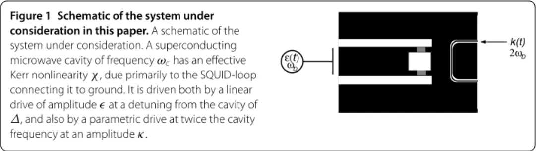
In recent experiments at Chalmers [], a quarter wave coplanar microwave cavity is terminated to ground via one or more superconducting quantum interference devices (SQUIDs), see Figure . By modulating the flux through the loop, the cavity frequency can be modulated. If the flux is varied at twice the cavity frequency this implements a para-metric driving of the cavity field. The cavity field also exhibits a large effective nonlinear susceptibility that can be modelled as an intensity dependent phase shift [].
Figure 1 Schematic of the system under consideration in this paper.A schematic of the system under consideration. A superconducting microwave cavity of frequencyωchas an effective Kerr nonlinearityχ, due primarily to the SQUID-loop connecting it to ground. It is driven both by a linear drive of amplitudeat a detuning from the cavity of
Δ, and also by a parametric drive at twice the cavity frequency at an amplitudeκ.
This paper is structured as follows. In Section we introduce the nonlinear microwave system considered in this paper. We establish a description in the form of a Markov mas-ter equation, one mas-term of which being an effective Hamiltonian we derive. We also give the input-output formulation of the microwave system. In Section we present a detailed analysis of the fixed point structure of the nonlinear microwave system in a semi-classical description, including bifurcation of the fixed points. We include dissipation of the mi-crowave mode. In Section we look at the steady state of the quantum system. This is done in a phase space representation based on the positive P-representation, both an-alytically, and numerically. We look for signatures of the semi-classical bifurcations. In Section we analytically compute and plot the small signal gain. Then, in Section we linearise the model and extract gain and noise spectra up to the threshold defined by the semi-classical bifurcation. Finally in Section we summarise our results.
A similar model to that considered here has been given by Wustmann and Shumeiko []. Their discussion of the semiclassical steady states and fixed point structure parallels the discussion here but gives a more detailed description of the semiclassical dynamics. They also discuss the quantum noise features of the model using a linearised quantum Langevin approach. In addition to a linearised analysis of the gain and signal-to-noise ratio, we give an exact steady state solution for the quantum master equation using the positive P-representation. The steady state behaviour of the model we describe has been experi-mentally observed by Wilson et al. [].
2 The dissipative Cassinian oscillator model 2.1 Master equation
We consider a superconducting microwave resonator connected through a superconduct-ing quantum interference device (SQUID) loop to ground. The SQUID loop consists of two separated Josephson junctions; a magnetic flux can then be applied to loop to change the effective resonant frequency of the cavity []. The SQUID also induces a significant quartic nonlinearity. Following Wallquist et al. [] we describe the integrated cavity + SQUID system in terms of an equivalent circuit composed of a capacitor and a nonlin-ear inductor. The Hamiltonian for one mode of the cavity field may be written in terms of this effective nonlinear oscillator as []
H=ECn+ELφ+λφ, ()
whereEC=(e)
C represents the charging energy of the effective LC oscillator whilenis the number of elementary charges on the capacitor,EL=
and on the mode function of the cavity fieldλ=ELB, whereBis a geometric factor. Further details are given in Wallquist et al. give [].
The system may be quantised by introducing the bosonic raising and lowering operators, defined in terms of the canonical variables of the cavity field as,
ˆ
φ=
EC EL
ˆ
a+aˆ†,
ˆ
n= –i
EL EC
ˆ
a–aˆ†,
()
whereψˆ andnˆare the average phase across the junctions and charge on the junctions, re-spectively andCandLare the effective lumped capacitance and inductance, respectively, of the equivalent circuit for the cavity in terms of which the cavity resonant frequency is give byωc=√LC. The total Hamiltonian, including the coherent driving and the paramet-ric driving are then given by
H=ωcaˆ†aˆ+
∗aˆeiωDt+aˆ†e–iωDt+χaˆ†aˆ+
κ∗aˆeiωDt+κaˆ†e–iωDt, ()
where ωc is the cavity frequency, =||eiυ represents the coherent driving strength,κ represents the parametric driving strength,ωDis the coherent driving frequency and we have assumed that the parametric driving is at twice the coherent driving frequency and
υ is the phase difference between the coherent driving and the parametric driving as we have taken the phase of the parametric driving term as zero. In Section we consider coherent homodyne detection of the cavity output. This means there is another phase in this problem; the phase choice for the local oscillator which may not be in phase with either the coherent or the parametric driving. The term proportional toχ represents a nonlinear (quartic) phase shift that arises from the nonlinear inductance of the SQUID loop. Quartic non-linearities in oscillators have been discussed in [, ]; parametric terms in the nano-electromechanical context have been discussed in [–].
For a realistic device we adopt a dissipative model. We model the microwave cavity res-onator as being damped in a zero temperature heat bath. Such a model for the bath is certainly justified as the typical microwave cavity is at mK temperature and thus the mean excitation photon number is very close to zero []. The amplitude decay rate for the mi-crowave cavity isγ. We then describe the dissipative dynamics with the master equation (with weak damping and the rotating wave approximation for the system-environment couplings). In an interaction picture at the coherent driving frequency this is
dρˆ
dt = – i
[Hˆ,ρˆ] +γ
aˆρˆaˆ†–aˆ†aˆρˆ–ρˆaˆ†aˆ, ()
whereρˆ is the density matrix of the microwave cavity, andHˆ is the Hamiltonian in an interaction picture in a rotating frame with respect to the linear driving frequency. We have made the rotating wave approximation by ignoring terms with frequency ωD or above. We thus have
ˆ
H=Δaˆ†aˆ+∗aˆ+aˆ†+
κ∗aˆ+κaˆ†+χ aˆ
†ˆ
whereΔ=ωc–ωD. In the absence of damping, classical trajectories arising from the para-metric and nonlinear portion of this Hamiltonian are the ovals of Cassini, and that system is hence sometimes described as the ‘Cassinian’ oscillator; the quantum version of that part of the Hamiltonian system has been previously studied by Wielinga et al. [] and more recently by Dykman and his collaborators [].
The semi-classical dynamics and the exact quantum steady state can be found using the complex P-function of Drummond and Gardiner []. In this approach the density operator in terms of the off diagonal projectors onto oscillator coherent states
ˆ
ρ(t) =
dαdβP(α,β,t)|αβ
∗|
β∗|α. ()
This function determines the normally ordered moments by
ˆ
a†maˆn=
dαdβP(α,β,t)αnβm. ()
It may seem surprising at first sight to notice that the Positive P-function has support in a phase space with twice as many canonical variables as the corresponding classical prob-lem. There is a direct physical interpretation of the extra variables based on a measurement model in which there are twice as many readout channels for the canonical phase space variable []. This is required if the distributions are to give normally ordered moments directly via integration. In [] a direct implementation using circuit QED of these addi-tional channels is demonstrated and connection is made to the stationary normal ordered moments.
The master equation can then be converted into a Fokker-Planck like equation for the P-function,
∂P(α,β)
∂t = ∂α
(γ+ iΔ)α+ i+ iχβα+ iκβ+∂β
(γ – iΔ)β– i∗– iχ αβ– iκ∗α
+∂αα
–i
κ+χ α+∂ββ
i
κ∗+χβ, ()
where∂α=∂α∂ and∂αα = ∂
∂α ∂αetc. The corresponding stochastic differential equations are
dα= –(γ + iΔ)αdt– idt– iχ α+κβdt+–iκ+χ α
dz
,
dβ= –(γ– iΔ)βdt+ i∗dt+ iχβ+κ∗αdt+iκ∗+χβ
dz
.
()
The semi-classical equations are obtained by settingβ=α∗in the drift term and ignoring the diffusion term, and are thus
dα
dt = –
γ+ iΔ+ iχ|α|α– i– iκα∗, ()
3 Semi-classical fixed point structure 3.1 No coherent driving,
= 0
We first consider the case of no driving field= . The semi-classical equations of motion () are then given by
dα
dt = –(γ+ iΔ)α– iχ α|α|
– iκα∗. ()
The semi-classical steady states,α=√neiθ, are given byn¯= , and
¯
n= –Δ±
κ– , sin(θ) = –
κ,
()
where we have defined the scaled variables
¯
n=
χ γn, κ=κ
γ,
Δ=Δ
γ.
()
In order to determine the stability of the fixed points, we linearise the equations of tion around the fixed points. Thus we have the semi-classical linearised equation of mo-tion forδα=α–αandδα∗=α∗–α∗
d(δα)
dt
d(δα∗) dt
≈Mαα∗
δα δα∗
, ()
where
Mαα∗=
–γ – iΔ– iχ|α| –iχ α– iκ
iχ(α∗)+ iκ –γ + iΔ+ iχ|α |
. ()
In the limit of no parametric pumping (κ= ), this Jacobian matches the result obtained by Babourina-Brooks et al. in []. Stability of the fixed point requires all the eigenvalues of the Jacobian to have a real part less than or equal to zero []. A real part of exactly zero indicates marginal stability in that parameter direction, where the fixed point is neither attractive nor repulsive. Real parts strictly less than zero are attracting fixed points which draw in nearby regions in phase space. In general, stability may depend on more coupling parameter combinations than those which define the fixed points.
The origin is a fixed point for all parameter values. Indeed, the origin is the only fixed point forκ<γ, the ‘below threshold’ regime. This fixed point is stable forκ<γ+Δ. Four additional fixed points occur as antipodal pairs for κ >γ; the ‘above threshold’ regime. The first additional pair of fixed points, which we will call the ‘stable pair’, and are given by
(n¯, θ) =
exists forΔ<(κ)–γ, and is always stable. The second additional pair of fixed points,
which we will call the ‘unstable pair’
(n¯, θ) =
–Δ–κ– , –arccscκ, ()
exists forΔ< –(ka)–γ, and is always unstable. We note that the unstable pair of fixed
points can only exist for negative detuning, and that whenever the unstable pair of fixed points exists, the first pair of fixed points exists also. Also, we note that for= ,aˆ→–aˆ is a symmetry of the system, and thus pairs of antipodal fixed points are the expected semi-classical result. We plot the radial and angular components of the semi-classical fixed points in Figure . The colour in these plots shows the stability.
The bifurcating behaviour of the semi-classical steady state is depicted in the ‘phase di-gram’ of Figure . There are two qualitatively different transitions that can take place in
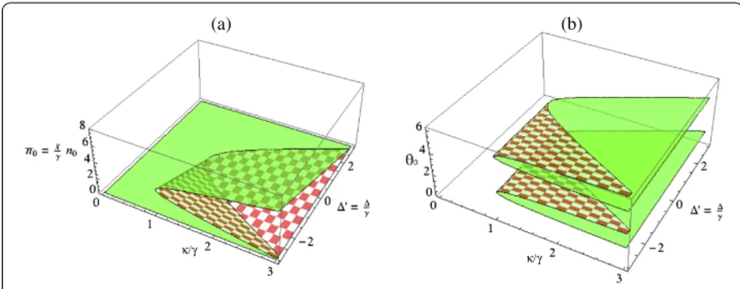
Figure 2 Radial and angular components of the semi-classical fixed points. (a)Radialn0¯ =χγn0and
(b)angularθ0components of the semi-classical fixed points. The existence and components of the
semi-classical fixed points are functions of the two non-dimensional ratios of the parametric pumping magnitudeκ, detuningΔ, and dissipation rateγof the system:κ=κγ andΔ=Δγ. Note then that all non-zero values in (a) represent not just a single fixed point, but a pair of antipodal fixed points. The fixed point at origin is not plotted in (b) for the obvious reason that its angular component is undefined. The colours of the plot indicate the stability: green indicates stable fixed points and checkered red indicates unstable fixed points. Visible in this diagram is a clear semi-classical threshold where the origin becomes unstable, and above which the stable semi-classical fixed points separate.
Figure 3 ‘Phase diagram’ of the semi-classical system.The ‘phase diagram’ of the semi-classical system. The existence and components of the semi-classical fixed points are functions of the two
non-dimensional ratios of the parametric pumping magnitudeκ, detuningΔ, and dissipation rateγof the system:κ=κγ andΔ
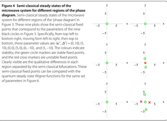
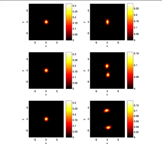
Figure 4 Semi-classical steady states of the microwave system for different regions of the phase diagram.Semi-classical steady states of the microwave system for different regions of the ‘phase diagram’ in Figure 3. These nine plots show the semi-classical fixed points that correspond to the parameters of the nine black circles in Figure 3. Specifically, from top-left to bottom-right, moving form left to right, then top to bottom, these parameter values are: (κ,Δ) = (0, 10), (5, 10), (0, 0), (5, 0), (0, –10), and (5, –10). The colours indicate stability; the green circle markers are stable fixed points, and the red cross markers are unstable fixed points. Clearly visible are the qualitative differences in each region separated by the semi-classical bifurcations. These semi-classical fixed points can be compared with the quantum steady state Wigner functions for the same set of parameters in Figure 6.
the semi-classical system as it moves from being ‘below threshold’ to ‘above threshold’. First, for positive detuning (Δ> ), the threshold parametric pumpingκ= is effectively increased by the detuning toκ=√ +Δ(the solid green/checkered red boundary in
Fig-ure . At this threshold, the semi-classical system undergoes a supercritical pitchfork bi-furcation where the stable origin goes unstable, and the stable pair of fixed points emerges from the origin and grows in separation with increasing parametric pumping (the check-ered red region in the upper half-plane in Figure ). Alternatively, for all values of negative detuning (Δ< ), at the threshold parametric pumpingκ= two saddle-node bifurca-tions produce both the stable and unstable fixed point pairs (the solid green/striped blue boundary in Figure ). The origin remains stable, and the two newly created pairs of fixed points then exist for parametric pumping above threshold (κ> ) until pumping reaches the even higher valueκ=√ +Δ. Between these two values (the striped blue region in
Figure ) with increasing parametric pumping, the stable pair increases in separation and the unstable pair moves to the origin. At the higher parametric pumpingκ=√ +Δ(the
striped blue/checkered red boundary in Figure ) the unstable pair annihilates in a sub-critical pitchfork bifurcation at the origin, and the origin becomes unstable for all higher parametric pumpingκ>√ +Δ. The stable pair of fixed points continues to grow in
separation with further increased parametric pumping (the checkered red region in the lower half-plane in Figure ).
We now illustrate the steady state behaviour of the semi-classical microwave system in different ‘phases’. We choose a point in parameter space from each region of the semi-classical ‘phase diagram’ of Figure . These choices are marked with the black circles in that figure. These steady states are shown in Figure . Some other near identical steady states, corresponding to the black crosses in Figure are depicted in Figure . These are plotted for comparison with the quantum version of the system in Section .
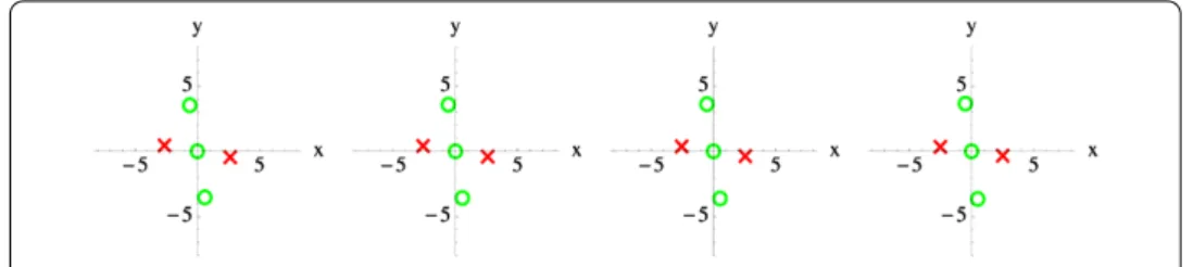
parame-Figure 5 Semi-classical steady states of the microwave system for different regions of the phase diagram.Semi-classical steady states of the microwave system for different regions of the ‘phase diagram’ in Figure 3. These eight plots show the semi-classical fixed points that correspond to the parameters of the eight black crosses in Figure 3. Specifically these parameter values, fro left to right, are:
(κ,Δ) = (3, –10), (3.25, –10), (3.5, –10), and (3.75, –10). The colours indicate stability; the green circle markers are stable fixed points, and the red cross markers are unstable fixed points. All fixed points in the same regions of parameter space are very similar qualitatively. These semi-classical fixed points can be compared with the quantum steady state Wigner functions for the same set of parameters in Figure 7.
ters: the magnitude of the parametric pumping rateκ; the detuningΔ; and the dissipation rateγ. And specifically, only the two non-dimensional ratios of them, here we choseκ=κ
γ andΔ=Δ
γ. Thus, the below threshold to above threshold transition of the parametric oscillator is independent of the size of the induced Kerr nonlinearityχ. However, the sep-aration of the semi-classical fixed points√n¯=
χ
γn, and thus the degree and visibility of the above-threshold oscillations, depends on the scaling parameter χγ. Thus, to see the semi-classical fixed points move significantly away from the origin, and thus to observe significant above-threshold behaviour we require a significantly large nonlinearityχ as well as parametric pumpingκ.
It will also prove useful to consider the non-dissipative limit (γ →) of the semi-classical equations on resonance (Δ→). The fixed points are no longer stable zero di-mensional attractors but rather elliptical fixed points corresponding to stable small os-cillations in the corresponding Hamiltonian model. One easily sees that the fixed points occur at
α= –κ
χ. ()
3.2 Including coherent driving,
= 0
Similar to our definitionsα=
√ ¯
neiθandn¯, we introduce the scaled Cartesian
coordi-natesx¯andy¯such thatα=x+ iyand
¯
x=
χ γx,
¯
y=
χ γy.
()
We also define the scaled linear driving
¯
=
χ γ
In terms of these, the fixed points of the semi-classical equation of motion () satisfy the quintic equation
= κy¯– ¯κ¯y+κ+Δκ–κ+¯y¯ + ¯Δ– κ+ ¯ + κΔ– κy¯ + +Δ–κ– ¯ ¯+ ¯Δ– κy¯
+¯+ ¯Δ+κ+ ¯. ()
We notice that were there to be only a small input signal and not a large linear drive with a small input signal on top (=¯= ), then the quintic factorises into the quadratic
=y¯
κy¯+ κ+Δκ–κy¯+ +Δ–κ. ()
This of course defines the tractable analytic fixed points given in Section ..
Unfortunately, solving a quintic equation analytically in terms of radicals can lead to un-helpful expressions, and is not even always possible. We can of course numerically solve for the fixed points for certain parameter values, but we leave non-perturbative explo-ration of the steady states of the= system for a later study. Instead, we will ultimately expand the Positive P function as a power series inin Section .
4 Quantum steady state
In the previous section we described the fixed point bifurcations of the semi-classical sys-tem. Here, we investigate whether there is a signature of those semi-classical bifurcations present in the full quantum system. This can be done exactly using the positive P func-tion, or numerically by computing the quantum steady state density operator in a trun-cated number basis and then constructing a phase space quasi probability density (e.g. a Q function) in different regions of the semi-classical ‘phase diagram’ of Figure . As we will show, by changing the coupling parameters so as to be on different sides of a semi-classical bifurcation, there is a corresponding qualitative change in the quantum steady state. This kind of correspondence principle has proven to be the case for other dissipative nonlinear quantum systems [–].
4.1 Steady state via the positive P function
The steady state solution of () can be found as the potential conditions are satisfied []. The steady state solution can be written as
Ps(α,β) =Ne–V(α,β), ()
where the potential function is given by
V(α,β) = –αβ–λlnχ α+κ–λ∗lnχβ+κ
–√
χ κarctan α
A
–
∗
√χ κ arctan β
where
λ= – +Δ
χ – i γ
χ, ()
andA=
–α=κ
χ determines the semi-classical fixed points of the corresponding Hamiltonian (non-dissipative) model, see (). This may be written in an alternate form by noting thatarctanx= iln–i+ixx,
Ps(α,β) =N
α–α
α+α
μ
α∗–β α∗+β
μ∗
χ α+κλχβ+κλ∗eαβ, ()
whereμ= i√
χ κ.
Before we can compare this distribution to the phase space structure of the semi-classical fixed points we must face the unusual feature that the Positive P function has support on a phase space with twice as many dimensions as the corresponding classical problem. The semi-classical subspace corresponds toβ=α∗. If it were not for the noise terms in the stochastic differential equations, (), we could start on this subspace and never leave it. The noise however will drive the dynamics off the semi-classical subspace. Despite this we can find a very close correspondence between the semi-classical fixed points and the form of the steady state Positive P function.
We first discuss the correspondence for the case of no coherent driving,= . The peaks of the steady state positive P function will be located at the minimum of the corresponding potential function, that is to say, the solutions of,∂αV=∂βV= . This gives
β= – λα
α–α
,
α= – λ
∗β
β–α∗
,
()
where we have used (). A little algebra shows that these are equivalent to
β–α∗α–α=|λ|, ()
– (αα)
– (α∗ β)
= λ
λ∗. ()
There are two classes of solutions:β=α∗andβ= –α∗. We will refer to the first of these as the semi-classical subspace and the second as the nonclassical.
We first consider the semi-classical subspace. Withβ =α∗, the first equation in () should be compared with the semi-classical steady state from (), which may be written as
α∗= –( Δ χ – i
γ χ)α
α+κ χ
. ()
In the limit of small quantum noise,χ→,κ→, such that κχ = constant we find that
λ≈ Δ
χ – i γ
and, in the semi-classical subspace, the P-function is peaked on the semi-classical steady states.
In the model of Wolinsky and Carmichael [] the nonlinear detuningχbecomes com-plex, thus describing nonlinear damping, and the dynamics of the positive P-function takes a very similar form to that considered here. In particular the additional fixed points of the non classical dimension are also present. As they describe, the non classical sub-space allows the noise to drive a stochastic process that corresponds to the nonclassical features of the steady state solution. In the case of strong nonlinearity they show that the steady state positive P-function on the non classical subspace is localised on the non clas-sical fixed points and that these peaks reflect the fact that the steady state is close to a superposition of two coherent states localised on the classical fixed points.
The explicit solutions to () are not straightforward; they are
(α,β) = (, ), ()
±
α∗
|α|+ iλ {λ} ±λ
|α|– {λ},
∓±
α
|α|– iλ∗ {λ} ±λ∗
|α|– {λ}
.
These are very close, though not exactly coincident, with the semi-classical fixed points derived in Section .
4.2 Numerical steady state
To perform the numerical computation of the quantum steady state we use the Quantum Optics MATLAB toolbox []. To do this we approximate the infinite basis of the mi-crowave cavity oscillator; we choose to do this by truncating in the Fock (number) basis. This means that we must choose couplings such that the bifurcation takes place suffi-ciently close to the origin to be accurately approximated by the truncation. This is roughly because a coherent state of amplitudeα has a mean occupation number of|α|. Given the quantum steady state typically (as we shall see direct evidence of in this section) has support centred on the semi-classical steady state, fixed points far from the origin (high
|α|) will produce high occupations and thus inaccurate results if we truncate in the Fock (number) basis.
We choose a point in parameter space from each region of the semi-classical ‘phase diagram’ of Figure . These choices are marked with the black circle markers in that figure. Semi-classically, the corresponding steady states were shown in Figure . We now look at the quantum steady state through the Wigner function of the steady state density matrix. The Wigner function is defined asW(x,y) =π–∞∞dzx–z| ˆρ|x+zeiyz; for more on the
Wigner function see [, ]. These Wigner functions are shown in Figure . There are clear signature of the semi-classical bifurcations. The quantum steady state has support centred on the stable semi-classical fixed points, something which has been previously observed in [–].
Figure 6 Steady state Wigner functions of the quantum microwave system.Density plots of steady state Wigner functions of the quantum microwave system for various parameter regimes. The Wigner function
W(x,y) is plotted wherexandyare two quadratures of the microwave field. These nine plots show the quantum steady states that correspond to the parameters of the nine black circles in Figure 3. Specifically, from top-left to bottom-right, moving form left to right, then top to bottom, these parameter values are: (κ,Δ) = (0, 10), (5, 10), (0, 0), (5, 0), (0, –10), and (5, –10). The other parameters are set to unityχ=γ= 1 for the purpose of having a Wigner density well inside the number basis truncation. The quantum steady state shows clear signs of the semi-classical bifurcations it undergoes. Particular comparison can be made to the semi-classical steady states of Figure 4. The quantum steady state has support centred on the semi-classical stable fixed points.
quantum steady states corresponding to small parameter changes in this region. In partic-ular, we look at the quantum steady states corresponding to the parameter space choices marked with black crosses in Figure . Semi-classically, the corresponding steady states were shown in Figure . The corresponding Wigner functions are shown in Figure . In-terestingly, there is a gradual transition from quantum steady state support centred on the semi-classical stable fixed point at the origin, to support centred on the separated sta-ble pair. This transition does not correspond to any semi-classical bifurcation, and at this stage is a quantum feature we cannot explain or predict semi-classically. We mention it here to suggest one direction for future investigation of this system.
5 The small signal gain
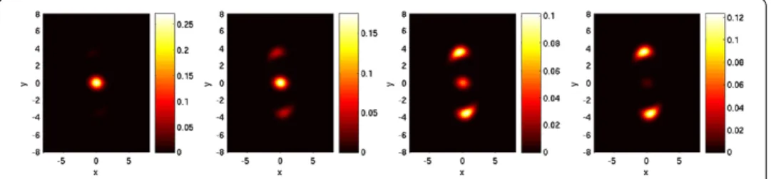
nor-Figure 7 Steady state Wigner functions of the quantum microwave system.Density plots of steady state Wigner functions of the quantum microwave system for small parameter changes in the blue parameter region of Figure 2. The Wigner functionW(x,y) is plotted wherexandyare two quadratures of the microwave field. These eight plots show the quantum steady states that correspond to the parameters of the eight black crosses in Figure 3. Specifically from left to right these parameter values are:
(κ,Δ) = (3, –10), (3.25, –10), (3.5, –10), and (3.75, –10). The other parameters are set to unityχ=γ= 1 for the purpose of having a Wigner density well inside the number basis truncation. Comparison should be made with the semi-classical steady states of Figure 5. The quantum steady state shows support that shifts from being centred on the semi-classical stable fixed point at the origin, to being centred on the separated stable pair. This transition does not correspond to any semi-classical bifurcation. While the semi-classical steady states of Figure 5 are quite insensitive to small parameter shifts in regions bounded by semi-classical bifurcations, the corresponding quantum steady states have a marked qualitative change.
malization constantN is fixed. To this end we define the integrals
Amn=N–
dαdβ αnβmPs(α,β), ()
and express the normally ordered moments as
ˆ
a†maˆn=Amn A
. ()
If we wish to regard this system as an amplifier, we need to calculate the mean cavity field amplitudeˆaas a function offor the case thatκ. With this in mind we expand the solution in a Taylor series in
Ps(α,β) =P()s (α,β) – μ
∞
k=
k+
α α
k+
P()s (α,β)
– μ∗ ∞
k=
k+
β α∗
k+
Ps()(α,β), ()
wherePs()(α,β) is the exact steady state solution for= . Then
Amn=A()mn– μ
∞
k=
k+
α α
k+
A()m,n+k+
– μ∗ ∞
k=
k+
β α∗
k+
A()m+k+,n. ()
If we now substitute () (with = ⇒μ= ) into (), and use the Beta function identity
– eiπ α – eiπβB(α,β) =
C
tα–( –t)β–dt, ()
then we obtain the moments for zero coherent driving
A()mn=κ
λ+λ∗+ – eiπ(λ+) – eiπ(λ∗+)
–χ
–κ
χ (n+m)/
×
∞
l=
l!
κ χ
l
+ (–)l+n + (–)l+m
×B
λ+ ,l+n+
B
λ∗+ ,l+m+
. ()
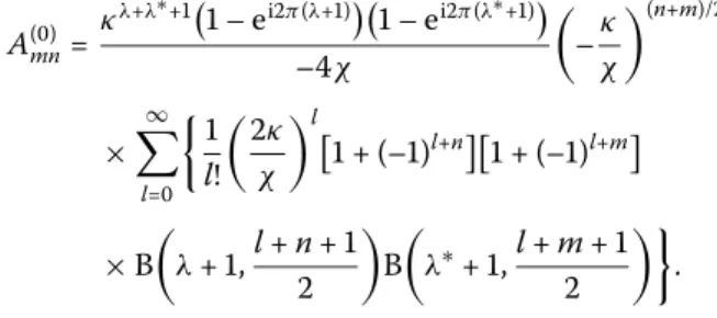
Since we will always be interested in ratios of these, we can omit the leading constant; this then exactly matches the expression found by Kryuchkyan and Kheruntsyan []
A()mn=
–κ
χ
(n+m)/∞
l=
l!
κ χ
l
+ (–)l+n + (–)l+m
×B
λ+ ,l+n+
B
λ∗+ ,l+m+
. ()
We first consider the steady state mean intra-cavity photon number with no coherent sig-nal,
ˆ
a†aˆ()=A
()
A()
. ()
In Figure we plot this as a function of the parametric driving strength. Note that we do not see a bistable curve as in Figure . The reason for this is that the quantum steady state gives a long time average which averages over all possible switching events between the two semi-classical steady states in the bistable region. The quantum steady state is a double peaked distribution in the complex P representation with each peak localised near one or the other semi-classical fixed points in the bistable region.
Figure 8 The steady state mean photon number in the cavity for no linear driving.The steady state mean photon number in the cavity for no coherent driving
= 0 as a function of the parametric pump magnitudeκ
and the detuningΔ. The corresponding semi-classical fixed points plotted in Figure 2 showed bi-stability for negative detuningΔ< 0 which does not occur in the quantum steady state. Time units are chosen so thatγ
We can now write the moments of the intra-cavity field as,
ˆ
a†maˆn=aˆ†maˆn()– μ ∞
k=
k+
α
k+
ˆ
a†maˆn+k+()
– μ∗ ∞
k=
k+
α∗ k+
ˆ
a†m+k+aˆn(), ()
where· · ·denotes the steady state average for= . In particular, the average amplitude
in the cavity at steady state is
ˆa=ˆa()– μ ∞
k=
k+
α
k+
ˆ
ak+()
– μ∗ ∞
k=
k+
α∗ k+
ˆ
a†k+aˆ(), ()
where we have usedˆa= . Explicitly, this average amplitude is
ˆa= –α N ∞ k= ∞ r= k+
r|α
|r
(r)!
+r
+r+k
×
μ
(+r+λ∗)(+r+k+λ)+
μ∗|α|
(+r+λ)(+r+k+λ∗)
, () where N= ∞ s=
s|α|s
(s)!
|(+s)|
|(+s+λ)| ()
we recall thatα= –κ
χ,λ= – + Δ χ – i
γ
χ, andμ= i
√χ κ = i√κ χ
|χ|. Writing=||e
iυ, we can obtain the magnitude of the cavity field at steady state|ˆa|,
ˆa=G
κ χ, Δ χ, γ χ,υ
χ, ()
where the gainG=G(κ χ,
Δ χ,
γ
χ,υ)≥ is
G= R ∞ k= ∞ r= k+
r (r)!
κ χ r +r
+r+k
× S– (κ χ)e –iυ S∗ , () where R= ∞ s=
s (s)!
κ χ
s |( +s)|
|(+s+Δχ – iχγ)|,
S=
+r+
Δ χ + i
γ χ
+r+k+
Δ χ – i
γ χ
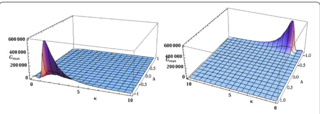
Figure 9 The maximum gain versus the pump magnitude and detuning.The maximum gain
Gmax= max{G}at the optimal signal phaseυ, versus the parametric pump magnitudeκand detuningΔ, with time units chosen so thatγ= 1 andχ= 0.25. The two plots show different camera perspectives of the same plotted data. The plot is made from summing 300 terms of the appropriate hypergeometric series. The summation is not normalised, and thus the gain values are only correct up to a scale; however, the shape of the plot is indicative.
Figure 10 The superconducting microwave resonator modelled as a single-sided cavity for use as an input-output formulation.
The superconducting microwave resonator modelled as a single-sided cavity for use as an input-output formulation. The incoming field mode operator isaˆi(t) and the outgoing field mode operator isaˆo(t). Loss from the microwave cavity occurs at a rateγ. Note here thatγis the coefficient of the amplitude decay, the coefficient for the photon
number loss is 2γ. The Hamiltonian dynamics of the cavity modeaˆare governed by the Interaction picture HamiltonianH.
In Figure we plot the maximum gainGmax=max{G} for a given parametric pump
strengthκand detuningΔ. We have plotted the maximum gain by choosing the optimal signal phaseυat each set of parameters. Comparing this to Figure for the case when there is no coherent driving, we see that the gain is a maximum around the critical parametric driving strength in the bi-stable, negatively detuned region.
6 Linearised quantum system 6.1 Input-output formalism
We consider the microwave cavity with the input-output formulation of quantum optics, as originally described by Collett and Gardiner in []. To do this, we model the super-conducting microwave resonator as a single-sided cavity as depicted in Figure .
The input and output fields are treated explicitly with their mode annihilation operators
ˆ
aiandaˆorespectively. With this formulation, the quantum stochastic differential equation we obtain for the microwave resonator field mode operatorsaˆandaˆ†are
daˆ dt = –
i
[aˆ,H] –γaˆ+
γaˆi(t),
daˆ† dt = –
i
ˆ
a†,H–γaˆ†+γaˆi†(t),
()
where the input field is effectively white noise, uncorrelated in time,
ˆ
ai(t),aˆi†
The probability per unit time to detect a photon in the input field is γˆai†(t)aˆi(t). Finally, the relationship between the input, output, and cavity fields is given by
ˆ
ao(t) =
γaˆ(t) + eiξaˆi(t), ()
where the phase of the second term, the reflected input, may vary with the system. For an almost perfectly reflecting mirror of an optical cavity we haveξ=πand eiξ= –, here we choose this phase as an appropriate approximation.
We also look at the various fields in the frequency domain, by defining the frequency-domain operators as the time-frequency-domain operators’ Fourier transforms,
ˆ˜
a(ω) =Ft→ω
ˆ
a(t),
ˆ˜
ai(ω) =Ft→ω
ˆ
ai(t)
,
ˆ˜
ao(ω) =Ft→ω
ˆ
ao(t)
,
()
where we have used the Fourier Transform convention ˜f(ω) = Ft→ω{f(t)} = √π×
∞
–∞dx f(t)e–iωt. In the frequency domain, the input field is also uncorrelated in frequency, ˆ˜
ai(ω),aˆ˜
†
i
ω=δω–ωIˆ, ()
and the relationship between the input, output, and cavity fields is then given by
ˆ˜
ao(ω) =
γaˆ˜(ω) –aˆ˜i(ω). ()
6.2 Gain spectra
Recall our quantum equations of motion for the microwave cavity field (). We linearise the system about a semi-classical fixed point αas we did semi-classically in (). This
gives us the linearised equation of motion for the fluctuation
⎡ ⎣d(
δa(t))
dt
d(δa†(t)) dt
⎤ ⎦=Mαα∗
δa(t)
δa†(t)
+γ
ˆ
ai(t)
ˆ
ai†(t)
, ()
where
δa(t) =aˆ(t) –α. ()
In the frequency domain the linearised equation of motion () becomes
iω δ˜a(ω)
˜
δa†(–ω)
=Mαα∗
˜
δa(ω)
˜ δa†(–ω)
+γ
ˆ˜
ai(ω)
ˆ˜
a†i(–ω)
. ()
We rewrite this to obtain an expression for the microwave cavity field fluctuation in terms of the input radiation,
˜
δa(ω)
˜ δa†(–ω)
=γ(iωI–Mαα∗)–
ˆ˜
ai(ω)
ˆ˜
a†i(–ω)
Using this expression, together with our input-output expression (), allows us to obtain an expression for the output fluctuation of the microwave cavity in terms of the input,
ˆ˘
ao(ω)
ˆ˘
a†o(–ω)
=G(ω)
ˆ˜
ai(ω)
ˆ˜
a†i(–ω)
, ()
where the gain matrixG(ω) is
G(ω) =
G(ω) G(ω)
G(ω) G(ω)
= γ(iωI–Mαα∗)––I. ()
Note thataˆ˘o(ω) is the output fluctuation in the frequency domain. If we re-introduced the coherent term we would obtain the full output amplitude in the frequency domain,
ˆ˜
ao(ω) =aˆ˘o(ω) +
√
π γ αδ(ω)ˆI.
Now, we can rewrite our JacobianMαα∗from () in terms of the parameters we defined in () for our semi-classical steady states,
Mαα∗=γ
– – i(Δ+ n¯) –in¯eiθ– iκ
in¯e–iθ+ iκ – + i(Δ+ n¯)
. ()
We now introduce two other useful parameters,∈R, andω∈R,
=
κ–Δ+n¯
–Δ+ κcos(θ) – n¯
,
ω=ω
γ.
()
In terms of these parameters, the gain matrixG(ω) is
G(ω) =
+ (ω– i)
×
– ––ω+ i(Δ+ n¯) in¯eiθ+ iκ
–in¯e–iθ– iκ – ––ω– i(Δ+ n¯)
. ()
To calculate the gain measured at an arbitrary phase, we first define the quadrature op-erator in the frequency domainXˆφ(ω) =aˆ˘o(ω)eiφ+aˆ˘
†
o(–ω)e–iφ, which can be written in terms of our gain matrix as
ˆ
Xφ(ω) =
eiφ e–iφG(ω)
ˆ˜
ai(ω)
ˆ˜
a†i(–ω)
. ()
This expression reduces to
ˆ
Xφ(ω) =gφ(ω)
ˆ˜
ai(ω)ei(φ+ζ(ω))+aˆ˜
†
i(–ω)e–i(
φ+ζ(ω)), ()
where our signal gaingφ(ω) at phaseφis
gφ(ω) =
|– ––ω– ie–iφ(κ+n¯e–iθ) + i(Δ+ n¯)|
+ (ω– i)
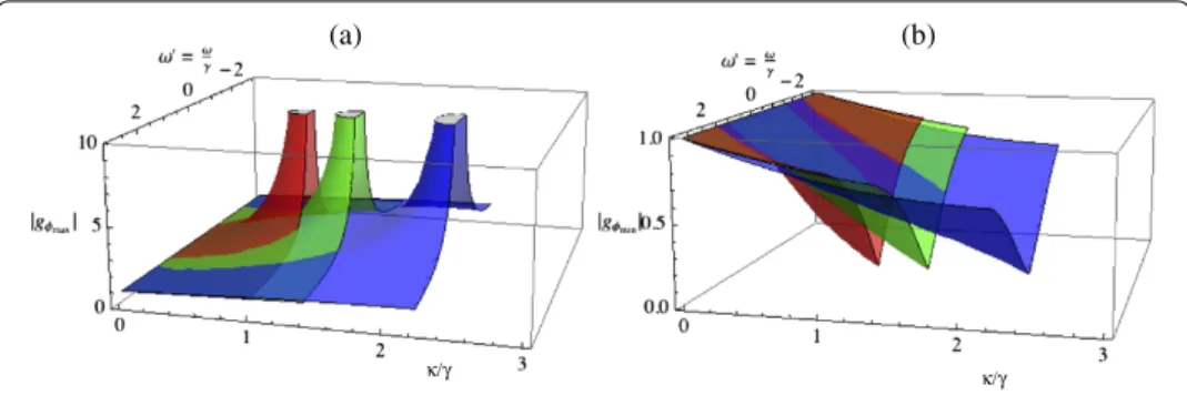
Figure 11 The maximum and minimum gain spectra. (a)The maximum gain spectra|gφmax(ω)|, and
(b)the minimum gain spectra|gφmin(ω)|, for linearisation about the fixed point at the origin for= 0. The gain is dependent upon four variables: the scaled parametric pumpingκ=γκ; the scaled detuningΔ=Δγ; and the scaled probed frequencyω=ωγ and phaseφ. Here, we plot the spectra against only the parametric pumping and the probed frequency. The different coloured sheets show different detunings: the red (innermost) surface shows the gain for no detuningΔ= 0; the green (central) surface shows the gain for
|Δ|= 1; and the blue (outermost) surface shows the gain for|Δ|= 2. Where the surface is not plotted (other than where it is truncated around the singularities at (κ2) = 1 +Δ2) it is because the origin does not exist as
a stable semi-classical fixed point to be linearised about for those parameter values. We choose the optimal phaseφto produce the (a) maximum gain, and (b) minimum gain, at DC for each pumping power and detuning.
and the frequency-dependent phase shiftζ(ω) is
ζ(ω) =arg– ––ω– ie–iφ
κ+n¯e–iθ
+ iΔ+ n¯
. ()
Note that while our signal gaingφ(ω) is complex for non-zero frequency, it is real for the DC frequency in this frame.
If we consider our analytically solved case of no linear driving bias ( =¯= ), and linearise about the ‘below threshold’ stable fixed point at the origin, then=κ–Δ<
and our gain|gφ(ω)|at a phaseφcan be plotted against the scaled parametric pumping
κand detuningΔ. We plot the maximum gain|gφmax(ω)|for each value of parametric pumping and detuning (optimisingφ to find the maximum gain at DC for each pair of these parameters) in Figure .
6.3 Squeezing spectra
Having derived the gain matrix () relating the input to the output, we are now also in a position to investigate the squeezing spectrum of the microwave system. Recall our quadrature operator in the frequency domainXˆφ(ω) =aˆ˘o(ω)eiφ+aˆ˘
†
o(–ω)e–iφ written in terms of our gain matrix in (). Our squeezing spectrum is the variance of this quadrature operator. We thus define this squeezing spectrumSφ(ω), again in the frequency domain, to be
Sφ(ω) =
∞
–∞ ˆ
Xφ(ω),Xˆφ
ωdω, ()
quadra-ture operator as
Sφ(ω) =
∞
–∞
eiφ e–iφG(ω)
ˆ˜ai(ω),aˆ˜i(ω) ˆ˜ai(ω),aˆ˜
†
i(–ω)
ˆ˜a†i(–ω),aˆ˜i(ω) ˆ˜a
†
i(–ω),aˆ˜
†
i(–ω)
×GωT
eiφ e–iφ
dω. ()
Then, using the commutation relation of () we can rewriteSφ(ω) in terms of normally-ordered variances of the input field as
Sφ(ω) =
∞
–∞
eiφ e–iφG(ω)
⎡ ⎢ ⎢ ⎣ ˆ˜
ai(ω),aˆ˜i(ω) ˆ˜a
†
i(–ω),aˆ˜i(ω) +δ(ω+ω)
ˆ˜a†i(–ω),aˆ˜i(ω) ˆ˜a
†
i(–ω),aˆ˜
†
i(–ω)
⎤ ⎥ ⎥ ⎦
×GωT
eiφ e–iφ
dω. ()
To proceed we now use the statistics of the input field. A coherent input field has zero normally-ordered variances (ˆ˜ai(ω),aˆ˜i(ω)=ˆ˜a
†
i(–ω),aˆ˜i(ω)=ˆ˜a
†
i(–ω),aˆ˜
†
i(–ω)= ). Thus, the only non-zero term in central matrix is the delta function term arising from the commutation relations. Using this, we can compute the integral of the matrix expres-sion, and our squeezing spectrum reduces to
Sφ(ω) =G(ω)G(–ω)eiφ+G(ω)G(–ω)
+G(ω)G(–ω) +G(ω)G(–ω)e–iφ, ()
or explicitly,
Sφ(ω) = |
– ––ω– ie–iφ(κ+n¯e–iθ) + i(Δ+ n¯)|
|+ (ω– i)|
. ()
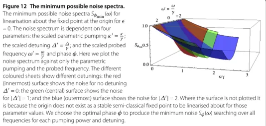
If we consider our analytically solved case of no linear driving bias ( =¯= ), and linearise about the ‘below threshold’ stable fixed point at the origin, then=κ–Δ<
and our squeezingSφ(ω) at a phaseφcan be plotted against the scaled parametric pumping
κand detuningΔ. We plot the squeezing spectrum for each value of parametric pumping and detuning (setting the phaseφto be that which gives the minimum noise searching over all frequencies for each pair of these parameters) in Figure .
6.4 Signal to noise ratio
For operation of the microwave system as a bifurcation amplifier, the parameters which re-sult in maximum gain may not rere-sult in minimum noise. Instead, rather than optimising for maximum gain or minimum noise individually, the quantity which we wish to max-imise is the signal to noise ratio. However, we see from our expressions for the gain () and noise (), thatSφ(ω) =|gφ(ω)|, and that our signal to noise ratio is thus unity,
SNRφ(ω) = | gφ(ω)|
Sφ(ω)
Figure 12 The minimum possible noise spectra.
The minimum possible noise spectraSφmin(ω) for linearisation about the fixed point at the origin for
= 0. The noise spectrum is dependent on four parameters: the scaled parametric pumpingκ=κγ; the scaled detuningΔ=Δγ; and the scaled probed frequencyω=ωγ and phaseφ. Here we plot the noise spectrum against only the parametric pumping and the probed frequency. The different coloured sheets show different detunings: the red (innermost) surface shows the noise for no detuning
Δ= 0; the green (central) surface shows the noise
for|Δ|= 1; and the blue (outermost) surface shows the noise for|Δ|= 2. Where the surface is not plotted it is because the origin does not exist as a stable semi-classical fixed point to be linearised about for those parameter values. We choose the optimal phaseφto produce the minimum noiseSφ(ω) searching over all
frequencies for each pumping power and detuning.
For the linearised system, this equality holds for all values of all parameters (parametric pumping, detuning, and cavity dissipation), all probed frequencies and phases, and re-gardless of which semi-classical fixed point we choose to linearise about.
Physically the means that our system is acting as a parametric amplifier. The quadrature of maximum gain is the same as the quadrature of maximum noise, and vice-versa for the minimum gain and noise. We can thus use this microwave system to amplify a signal to a measurable level without affecting its signal to noise ratio.
7 Conclusion
In this paper we detailed the quantum and semi-classical structure of a superconducting microwave resonator connected through a SQUID loop to ground. In particular we ob-served that the semi-classical model contains a bifurcation structure, and that the remains of this structure are still visible in the full quantum mechanical steady state. Furthermore, we showed it can be used as a bifurcation amplifier. We did this analysis by: linearising about the semi-classical steady state below the ‘threshold’ of the amplifier; by truncating the oscillator basis in the Fock basis and numerically computing the quantum phase space at steady state; and also by computing the exact quantum steady state by using an analytical phase space technique.
First, we showed that the corresponding semi-classical model has its fixed points deter-mined by a quintic polynomial. We showed that for the small linear signal regime= , that this quintic factors and is analytically solvable. This semi-classical system then un-dergoes a bifurcation of its semi-classical steady state with increased parametric pumping power. This bifurcation gives a threshold for the amplifier and occurs when the para-metric pumping power equals the cavity decay, with adjustment for a detuned drive,
|κ|=γ+Δ. The sign of the detuning specifies the form of the bifurcations. For a positive detuningΔ≥, the origin undergoes a supercritical pitchfork bifurcation at the thresh-old. For negative detuningΔ< , the origin instead loses its stability at|κ|=γ+Δin
In addition to numerically computing the quantum phase space at steady state by trun-cating the oscillator basis, we also calculated the exact quantum steady state. This was done following the work of Kryuchkyan and Kheruntsyan [] by using the Positive P representation. The method took advantage of the fact that the potential conditions were satisfied. The exact quantum phase space density at steady state was seen to be peaked in the vicinity of the corresponding semi-classical fixed points.
We showed that the quantum device functioned as a bifurcation amplifier until thresh-old. We calculated the small signal gain of the amplifier using the exact quantum steady state. We also approximated this by linearising the steady state about the semi-classical below-threshold fixed point using the input-output formalism of Collett and Gardiner []. With this procedure we also calculated noise spectra, and we showed that the signal to noise ratio at all frequencies and phases was equal to unity. We thus showed that the quarter-wave microwave resonator considered can be made to act as a parametric ampli-fier. This device can take a signal from a nano-electromechanical system and amplify it to a measurable level without affecting its signal to noise ratio.
Competing interests
The authors declare that they have no competing interests.
Authors’ contributions
The paper was written by CPM who did the numerical simulations and, together with GJM, performed the analytic calculations. HN obtained the solution in Section 4. TD provided some of the experimental parameters.
Author details
1Department of Physics, The University of Queensland, St Lucia, QLD 4072, Australia.2Department of Physics, Texas A & M
University at Qatar, PO Box 23874, Doha, Qatar.3Department of Physics, The University of New South Wales, Kensington,
NSW 2052, Australia.
Acknowledgements
This work was supported by the Australian Research Council grants FF0776191 and CE110001014.
Received: 29 January 2014 Accepted: 24 April 2014 Published: 10 June 2014
References
1. Devoret MH, Girvin S, Schoelkopf R:Ann. Phys.2007,16:767-779. doi:10.1002/andp.200710261. 2. Schoelkopf RJ, Girvin SM:Nature2008,451:664-669. doi:10.1038/451664a.
3. Sandberg M, Wilson CM, Persson F, Bauch T, Johansson G, Shumeiko V, Duty T, Delsing P:Appl. Phys. Lett.2008, 42:203501. doi:10.1063/1.2929367.
4. Wallquist M, Shumeiko VS, Wendin G:Phys. Rev. B2006,74:224506. 5. Wustmann W, Shumeiko V:Phys. Rev. B2013,87:184501.
6. Wilson CM, Duty T, Sandberg M, Persson F, Shumeiko V, Delsing P:Phys. Rev. Lett.2010,105:233907. 7. Kozinsky I, Postma HWC, Kogan O, Husain A, Roukes ML:Phys. Rev. Lett.2007,99:207201.
doi:10.1103/PhysRevLett.99.207201.
8. Babourina-Brooks E, Doherty A, Milburn GJ:New J. Phys.2008,10:105020. doi:10.1088/1367-2630/10/10/105020. 9. Woolley MJ, Doherty AC, Milburn GJ, Schwab KC:Phys. Rev. A2008,78:062303. doi:10.1103/PhysRevA.78.062303. 10. Hertzberg JB, Rocheleau T, Ndukum T, Savva M, Clerk AA, Schwab KC:Nat. Phys.2010,6:213.
11. Rocheleau T, Ndukum T, Macklin C, Hertzberg JB, Clerk AA, Schwab KC:Nature2010,463:72.
12. Wallraff A, Schuster DI, Blais A, Frunzio L, Huang R-S, Majer J, Kumar S, Girvin SM, Schoelkopf RJ:Nature2004,431:162. 13. Wielinga B, Milburn GJ:Phys. Rev. A1993,48:2494. doi:10.1103/PhysRevA.48.2494.
14. Marthaler M, Dykman M:Phys. Rev. A2006,73:042108.
15. Walls DF, Milburn GJ:Quantum Optics. 2nd edition. Berlin: Springer; 2008. 16. Braunstein SL, Caves CM, Milburn GJ:Phys. Rev. A1991,43:1153. 17. Eichler C, Bozyigit D, Wallraff A:Phys. Rev. A2012,86:032106.
18. Hilborn RC:Chaos and Nonlinear Dynamics. Oxford: Oxford University Press; 1994.
19. Hines AP, Dawson CM, McKenzie RH, Milburn GJ:Phys. Rev. A2004,70:022303. doi:10.1103/PhysRevA.70.022303. 20. Meaney CP, Duty T, McKenzie RH, Milburn GJ:Phys. Rev. A2010,81:043805. doi:10.1103/PhysRevA.81.043805. 21. Meaney CP, McKenzie RH, Milburn GJ:Phys. Rev. E2011,83:056202.
22. Carmichael HJ:Statistical Methods in Quantum Optics 1. Berlin: Springer; 2008. 23. Wolinsky M, Carmichael HJ:Phys. Rev. Lett.1988,60:1836.
24. Tan SM:Quantum optics and computation toolbox for MATLAB; 2002. 25. Zachos CK, Fairlie DB, Curtright TL (Eds): World Scientific.
doi:10.1140/epjqt7