802.11 with Multiple Antennas for Dummies
Daniel Halperin
∗, Wenjun Hu
∗, Anmol Sheth
†, and David Wetherall
∗†University of Washington∗and Intel Labs Seattle†
This article is an editorial note submitted to CCR. It has NOT been peer reviewed. The authors take full responsibility for this article’s technical content. Comments can be posted through CCR Online.
ABSTRACT
The use of multiple antennas and MIMO techniques based on them is the key feature of 802.11n equipment that sets it apart from earlier 802.11a/g equipment. It is responsible for superior performance, reliability and range. In this tu-torial, we provide a brief introduction to multiple antenna techniques. We describe the two main classes of those tech-niques, spatial diversity and spatial multiplexing. To ground our discussion, we explain how they work in 802.11n NICs in practice.
Categories and Subject Descriptors
A.1 [General Literature]: Introductory and Survey
General Terms
Design, Experimentation
Keywords
MIMO, 802.11n, Multiple Antennas
1.
INTRODUCTION
The use of multiple antennas at the receiver and trans-mitter has revolutionized wireless communications over the past decade. It has long been known that multiple receive antennas can improve reception through the selection of the stronger signal or combination of individual signals at a receiver. In the mid 1990s, however, seminal research by Foschini, Gans [2] and Telatar [7] predicted large perfor-mance gains from using multiple antennas atboth transmit-ter and receiver. This kind of system is called a MIMO (Multiple-Input Multiple-Output) system in contrast with a SISO (Single-Input Single-Output) system that uses one transmit antenna and one receive antenna. SIMO and MISO systems also exist, as we will see shortly.
The excitement around MIMO is that, for richly scattered wireless environments such as an indoor 2.4 or 5 GHz 802.11 LAN, the multiple antenna pairs can provide independent spatial paths between the transmitter and receiver. This spatial degree of freedom changes the fundamental relation-ship between power and capacity per second per Hz. Shan-non capacity increases by up to one bit/sec/Hz for every doubling of power. With N antennas at each end, however, capacity increases by up to N bits/sec/Hz for every doubling of power. That is,simply adding antennas has the potential to linearly scale the capacity even though the antennas trans-mit and receive on the same frequency band at the same time.
This is a key result in the quest for speed in modern wireless systems, since available spectrum is scarce and added power yields diminishing returns. Over the past decade, MIMO techniques have proved that they can deliver this value in practice. Today most high-rate wireless systems use MIMO technologies, including 802.11n, 4G mobile phone technology under the name LTE, and WiMAX.
Our aim in this note is to introduce multiple antennas as they are used in 802.11n wireless LANs to networking researchers with little previous knowledge of wireless com-munications. We choose 802.11n to ground the discussion in a relevant technology, but most of our discussion applies broadly to MIMO wireless systems. 802.11n is an extension of the earlier 802.11a/g standard that adds the use of mul-tiple antenna techniques at the physical layer. The IEEE ratified the 802.11n standard [1] in September 2009, but the physical layer details have been finalized for years. Draft 802.11n hardware has been commercially available since 2007 and now ships standard in many devices.
The way 802.11n uses multiple antennas is quite different than earlier 802.11a/g access points (APs) that had multiple antennas sticking out of the box. Those APs would typi-cally choose the best antenna to send or receive a packet, but still use a single antenna at a given moment. In terms of wireless signal processing, they are still SISO systems. With 802.11n, multiple antennas at the transmitter and/or receiver are used at the same time (and on the same fre-quency band). To enable this, transmitters and receivers must have multiple RF processing chains to go with their multiple antennas; the techniques used aresignal processing techniques implemented in the physical layer hardware with some amount of high-level control available to the driver. This processing is the hallmark of a MIMO system.
There are two basic classes of multiple antenna techniques that are described in textbooks and used in 802.11n.Spatial diversity techniques increase reliability and range by send-ing or receivsend-ingredundantstreams of information in parallel along the different spatial paths between transmit and re-ceive antennas. The use of extra paths improves reliability because it is unlikely that all of the paths will be degraded at the same time. Improved range, and some performance increase too, comes from the use of multiple antennas to gather a larger amount of signal at the receiver. In con-trast, spatial multiplexing techniques increase performance by sending independent streams of information in parallel along the different spatial paths between transmit and re-ceive antennas. This improves performance because, if we take care in how we construct and decode signals, adding
an antenna and independent stream of information need not slow down the streams that are already being sent.
We describe basic techniques for both these classes that are compatible with 802.11n and used in commercial NICs to the best of our knowledge. The 802.11n standard does not give any of the techniques per se because, as a standard, it is concerned with interoperability rather than implementation. It also contains rather a lot of options and we have focused on those options that are most commonly used today.
To put the role of multiple antennas in 802.11n in context, consider that the highest data rate in 802.11a/g is 54 Mbps and the highest data rate in 802.11n is 600 Mbps. This is an increase of a factor of 11. Of this, a factor of four comes from the use of four antennas. This forms the bulk of the increase and is easily the largest single factor. Another factor of two comes from simply using double width channels of 40 MHz instead of 20 MHz. The remaining improvement, about 40%, comes from tweaking the OFDM and coding constants to shave overhead. In practice, many devices may not have four antennas. Up to three antennas are commonly supported by NICs, and it is expected that clients will tend to have fewer antennas for space and power reasons, while APs will tend to have more antennas for performance reasons.
The rest of this tutorial is organized as follows. We begin with a quick discussion of an 802.11 wireless link in the sin-gle antenna case. Here, fading wireless channels are the key difficulty that the physical layer overcomes through the use of diversity techniques. We then describe how spatial diver-sity schemes add to the picture, from the simple selection of antennas as can be done with SISO processing to com-bining that requires a SIMO (or MISO) system. Next, we describe spatial multiplexing schemes, from simple direct-mapped MIMO to the use of precoding to extract larger gains in practice. We conclude with pointers to more ad-vanced techniques and other introductory material for the interested reader.
2.
WIRELESS CHANNELS & SISO 802.11
We begin with background on indoor wireless channels at 2.4 GHz and 5 GHz, and how single antenna 802.11 systems send information over these channels at the physical layer.
2.1
Faded Wireless Channels
In wireless communications, the performance of a link is fundamentally determined by the Signal-to-Noise Ratio (SNR), which measures the received signal strength of a transmission relative to the thermal noise in the receiver hardware that distorts the received signal. Over a typical 802.11a link today, packets are transmitted with 50 mW of power, and for a strong link the received power might be as high as 50 pW, a billion-fold loss (90 dB) of power. This re-ceived signal is still much greater than the noise floor, which for a 20 MHz 802.11 channel is about 0.1 pW. Thus the high SNR (10 log10(50/0.1)≈27 dB) supports a fast bit rate.
The weakening, orattenuation, of the signal between trans-mitter and receiver comes from several effects. One funda-mental effect ispath loss: as the radiated signal spreads out over a wider area, its power will spread out over the surface of a sphere (for a perfectomnidirectional antenna) or other geometric shape (fordirectional antennas). Path loss thus causes the power to drop off at least as fast as the square of the distance traveled. Otherfading effects cause the sig-nal to be weakened beyond the path loss. For example, just
as a tall building will block the sun, obstacles such as wa-ter, metal, and glass surfaces can prevent the radio waves from passing through. Analogous to visible light, this effect is calledshadowing. Path loss and shadowing are examples of macro effects that cause slow fading in which the sig-nal strength varies slowly over time as the receiver moves or the environment changes. Conceptually, moving around in a shadow behind a tall building will not greatly change the amount of sunlight (provided you stay in the shadow), nor will movements much less than the distance from the transmitter affect the path loss.
The most problematic kind of fading for 802.11 is due to multi-path. At 2.4 GHz and 5 GHz, RF signals bounce off metal and glass surfaces that are common indoors. This scat-teringleads to a situation in which many copies of the signal arrive at the receiver having traveled along many different paths. When these copies combine they may add construc-tively, giving a good overall signal, or destrucconstruc-tively, mostly canceling the overall signal, all depending on the relative phases of the portions. Measurement studies of fading re-port signal variations as high as 15–20 dB [4].
Worse yet, small changes in path lengths can alter the sit-uation from good to bad because the wavelengths at 2.4 GHz and 5 GHz (over which the RF signals go through a com-plete phase) are only 12 cm and 6 cm, respectively. Statisti-cal models tell us that multi-path fading effects are indepen-dent for locations separated by as little as half a wavelength. This means that multi-path causes rapid signal changes or fast fadingas the receiver moves, or in the case of a station-ary node as the surrounding environment changes. Because multi-path effects depend on the phases of signals, they are stronglyfrequency selective. This means that some unlucky frequencies in a 20 MHz 802.11 channel may be wiped out while others are unaffected. We will see an example in the next section.
The net effect of multi-path fading is that the received wireless signal can vary significantly over time, frequency and space. This is a problem for good performance because at any given time there is a significant probability of a deep fade that will reduce the SNR of the channel below the level needed for a given communication scheme.
2.2
Single Antenna 802.11 OFDM
The main technique used in wireless systems such as 802.11 to cope with variable wireless channels is diversity. Diver-sity is the spreading of information with some redundancy across multiple independently faded channels. When this is done, it is unlikely that a deep fade on a single channel will prevent successful communication. The trick, however, is to find independently faded channels. These exist within the physical layer and come from harnessing the time, frequency and spatial resources of the wireless link.
The 802.11a/g/n physical layer is based on OFDM (Or-thogonal Frequency Division Multiplexing). OFDM parti-tions the relatively wideband 20 MHz 802.11 channel (or carrier) into 64subcarriersof 312.5 kHz each, such that each subcarrier can be thought of as its own narrowband chan-nel. OFDM is completely different than the spread spec-trum technique used in older 802.11b equipment. There are many variations on OFDM, but data in 802.11 is sent on the subcarriers using the same modulation, coding scheme, and transmit power for each. This modulation ranges from BPSK, to QPSK, QAM-16 and QAM-64, with each higher
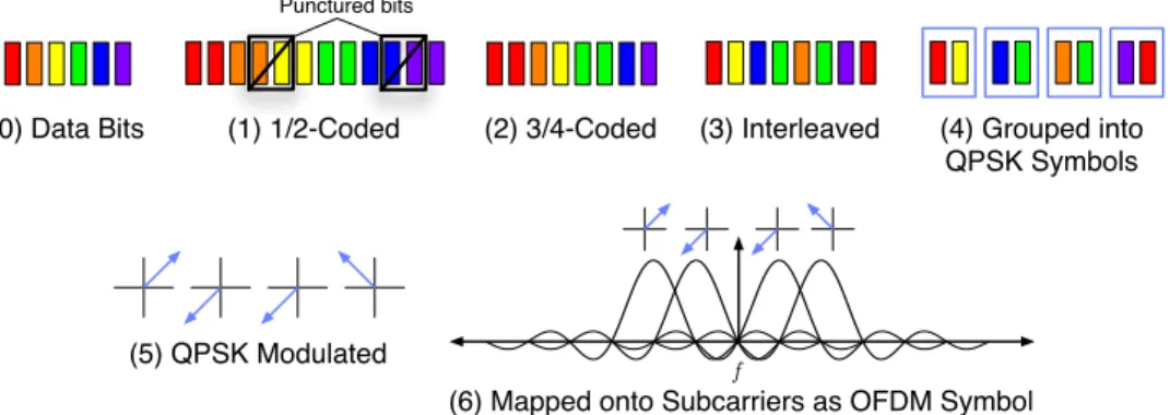
(5) QPSK Modulated f
(6) Mapped onto Subcarriers as OFDM Symbol (0) Data Bits (2) 3/4-Coded (3) Interleaved (4) Grouped into
QPSK Symbols (1) 1/2-Coded
Punctured bits
Figure 1: A graphical view of the OFDM encoding process for the 18 Mbps rate (QPSK, 3/4) of 802.11a. The data bits (0) are encoded by a rate-1/2convolutional code (1) and then optionally punctured by dropping certain bits for higher coding rates (here,3/4) that send fewer redundant bits (2). The remaining bits are in-terleaved (3) to spread the redundancy across subcarriers and protect against frequency-selective fades. These bits are grouped into symbols (4) based on the modulation (QPSK encodes2bits per symbol), modulated (5), and finally mapped onto the different subcarriers to form an OFDM symbol (6).
h11
h12
h11
h12
y = 2 x
Tx Rx
y = x
x 1
(a) Receive diversity
h11
h21
h11 h21
Tx Rx
x
x
( + ) x y =
y (b) Transmit diversity
x1
x2
h11
h12
h21
h22
h11x1 h21x2
h12x1 h22x2
y2 = +
Tx Rx
y = 1 +
(c) Spatial multiplexing
Figure 2: Using some of the transmit/receive antennas in an example 2x2 system to exploit diversity and multiplexing gain. xi and yi represent transmitted and received signals. The channel gain hij is a complex
number indicating a signal’s attenuated amplitude and phase shift over the channel between theith transmit antenna and the jth receive antenna. The received signalsyi will additionally include thermal RF noise.
modulation sending more bits per symbol and being used when there is a higher SNR. There are minor differences be-tween 802.11a/g and 802.11n. In 802.11a/g there are 48 data subcarriers, 4 pilot tones for control, and 6 unused guard subcarriers at each edge of the channel. In 802.11n, there are only 4 guard subcarriers at each edge of the channel, and two adjacent 20 MHz channels can be merged into a single 40 MHz channel.
The beauty of OFDM is that it divides the channel in a way that is both computationally and spectrally efficient. High aggregate data rates can be achieved, while the en-coding and deen-coding on different subcarriers can use shared hardware components. More relevant to our point here, how-ever, is that OFDM transforms a single large channel into many relatively independently faded channels. This is be-cause multi-path fading is frequency selective, so the differ-ent subcarriers will experience differdiffer-ent fades. Some adja-cent subcarriers may be faded in a similar way, but the fading for more distant subcarriers is often uncorrelated. Dividing the channel also increases the symbol time per channel, since many slow symbols will be sent in parallel instead of many fast symbols in sequence. This adds time diversity because the channel is more likely to average out fades over a longer period of time.
802.11 makes use of the frequency diversity provided by OFDM by coding across the data carried on the subcarriers. This uses a fraction of them for redundant information that can later be used to correct errors that occur when fading reduces the SNR on some of the subcarriers. First, a
con-volutional code of rate 1/2 adds redundant information. It is then punctured [3] by removing bits as needed to support coding rates of 2/3 and 3/4, plus 5/6 for 802.11n. At a rate of 3/4, for example, a quarter of the data on the subcarriers is redundant. An alternative LDPC (Low-Density Parity-Check) code with slightly better performance can also be used for 802.11n. Figure 1 presents a pictorial overview of the OFDM encoding process.
The net effect of OFDM plus coding is to provide consis-tently good 802.11 performance despite significant variabil-ity in the wireless signal due to multi-path fading.
3.
SPATIAL DIVERSITY
In this section we look at spatial diversity techniques that can be applied at the receiver and at the transmitter. Adding multiple antennas to an 802.11n receiver or transmitter pro-vides a new set of independently faded paths, even if the antennas are separated by only a few centimeters. This adds spatial diversity to the system, which can be exploited to improve resilience to fades. There is also a power gain from multiple receive antennas because, everything else be-ing equal, two receive antennas will receive twice the signal. These factors combine to improve performance at a given distance, and hence increase range.
3.1
Receive Diversity Techniques
Consider the arrangement in Figure 2(a). One transmit antenna at a node is sending to two receive antennas at a
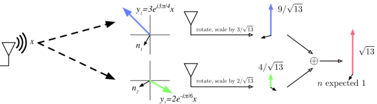
sec-n2
y2=2e-iπ/6x
rotate, scale by 2/√13 rotate, scale by 3/√13
⊕
9/√13
4/√13
√
13
x
n expected 1
y1=3ei3π/4x
n1
Figure 3: MRC operation on a sample channel. The channel gains are~h= h3ei3π/4,2e−iπ/6i, with Gaussian noise~n=hn1, n2i of expected power1. The antennas have respective SNRs of9 and 4. To implement MRC, the receiver multiplies the received signal~y=~hx+~n by the unit vector~h∗/||~h||, where~h∗ denotes the complex conjugate of ~h. This operation scales each antenna’s signal by its magnitude, and rotates the signals into the same phase reference before adding them. (For graphical clarity, we depict the common phase vertically, rather than at 0). The resulting sum has magnitude √13, and expected noise power1 because the scaling is normalized. Thus, by coherently combining received signals from different antennas, the MRC output has the expected SNR of13. In systems with OFDM, MRC is performed separately for each subcarrier.
ond node. This is known as a 1x2 system. Real systems may have more than two receive antennas, but two will suffice for our explanation. With this setup, each receive antenna re-ceives a copy of the transmitted signal modified by the chan-nel between the transmitter and itself. The chanchan-nel gains hij are complex numbers which entail both the amplitude
attenuation over the channel as well as the path-dependent phase shift. The receiver measures the channel gains based on training fields in the packet preamble. Note that the gains differ for each subcarrier (in frequency-selective fad-ing) as well as for each antenna. The question now is how to combine the two received signals to make best use of them. We consider two diversity techniques to show the extremes. The simplest method is to use the antenna with the strongest signal (hence the largest SNR) to receive the packet and ig-nore the others. We will call this method SEL, forselection combining. This is essentially what is done by 802.11a/g APs with multiple antennas. It helps with reliability, because both signals are unlikely to be bad, but it wastes perfectly good received power at the antennas that are not chosen.
The better method is to add the signals from the two antennas together. However, this cannot be done by simply superimposing their signals, or we will have just recreated the effects of multi-path fading. Rather, the signals should each be delayed until they are in the same phase; then, the power in the signals will combine coherently. To do this, the receiver needs a dedicated RF chain for each antenna to process the signals. This increases the hardware complexity and power consumption, but yields better performance.
As a twist in the above, the signals are also weighted by their SNRs. This gives less weight to a signal that has a larger fraction of noise, so that the effects of the noise are not amplified. The result is maximal-ratio combining, or MRC. MRC is known to be optimal (it is equivalent to a matched filter), and produces an SNR that is the sum of the component SNRs. Note that in frequency-selective fad-ing, this process is performed differently for each subcarrier according to its specific channel gains.
Figure 3 depicts MRC operation graphically for a 1x2 channel. In this example, the two channel gains have
magni--25 -20 -15 -10 -5 0
-20 -10 0 10 20
Normalized power (dB)
Subcarrier index
A C B and SEL AB (MRC) ABC (MRC)Figure 4: Frequency-selective fading over testbed links: the figure shows, for an example 5.2 GHz link, the received power measured on each subcarrier for individual antennas and under SEL and MRC diver-sity, normalized to the strongest subcarrier power.
tudes of 3 and 2. With expected noise power 1, these gains correspond to SNRs of 9 and 4, given that a signal’s power is the square of its magnitude. The MRC receiver scales each antenna’s signal by its magnitude, normalized to the total; delays the signals to a common phase reference; and then adds them. The result has magnitude√13, and the normal-ized weighted sum of noise still has expected power 1. The combined signal thus has a resulting sum SNR of 13.
As an example of how MRC and SEL work in 802.11, con-sider Figure 4. This figure shows the wireless signal strength of each subcarrier using three antennas for a real 802.11n link in our indoor wireless testbed. The subcarrier strengths are measured in decibels normalized to the strongest subcarrier strength. This figure gives a much more detailed view than metrics such as the RSSI (Received Signal Strength Indi-cation) for a link, which gives only the sum of the signal strength over all subcarriers.
For each antenna labeled A, B, or C, the signal varies over the channel, changing gradually from one subcarrier to the next. It shows some deep fades due to (frequency-selective) multi-path, particularly at antenna A which sees at least 20 dB (100×) of variation in subcarrier strengths. These deep fades will cause errors, since 802.11 uses the same technique for all subcarriers. Coding across the subcarriers will have to repair these errors for successful reception.
Figure 4 also shows how SEL and MRC perform on the received signals. Antenna B has the strongest overall signal and is hence chosen by SEL. However, its strength still varies over its subcarriers due to multi-path fading, in this case by 15 dB. This means that SEL can avoid unlucky antennas that are weak overall, but does little to improve on anten-nas that already have reasonable signals but have frequency-selective fades.
In contrast, MRC adds the signals (weighted by their SNR) for each subcarrier. This produces the top line on the figure that is better than each individual antenna at ev-ery point and significantly flatter over the channel. Now, the fading has been reduced to roughly 5 dB. This in turn means that coding will have to deal with fewer and less pro-nounced errors, which allows less redundant coding or higher modulation rates. MRC can produce significant diversity gains in practice that exceed the gains of antenna selection. Though receiver processing algorithms are not specified by the 802.11n standard, MRC is closely tied to MIMO signal decoding and is likely to be available in any 802.11n NIC.
3.2
Transmit Diversity Techniques
The receive diversity techniques we have looked at use a single transmit and multiple receive antennas. There are also transmit-side equivalents that use multiple transmit and single receive antennas. A 2x1 setup is shown in part (b) of Figure 2. This can be useful when the AP has more antennas than the client, so that it can use its multiple antennas to benefit a single antenna client.
The transmit-side equivalent of SEL is simply to select the single best antenna on which to transmit a packet. The transmit-side equivalent of MRC is a kind oftransmit beam-forming. The transmitter precodes the signals by delaying them to change the phase such that they combine construc-tively at the receiver’s antenna, and weighting them such that transmit power is allocated to each spatial path by its SNR. These techniques are the direct analogues of the receiver-side techniques.
The disadvantage of transmit diversity compared to re-ceive diversity is that the transmitter must know the chan-nel beforehand in order to select between antennas or to pre-code the signals. This requires feedback from the receiver, i.e. RSSI or packet delivery statistics to inform selection and channel gains to inform precoding. In 802.11n, there are an-tenna selection, rate selection, and channel state feedback packets that the receiver can use to send information to the transmitter. Alternatively, since the properties of RF chan-nels are reciprocal, the transmitter can learn the channel gains when it receives a packet from the target receiver. In practice, some calibration is needed to account for the differ-ing properties of the NICs at each end. In both cases, regular updates are needed because the channel state changes over time, often very quickly due to multi-path fading, and out-of-date channel gains make precoding less effective.
It is also worth noting that there are different
beamform-Method Capacity (bits/sec)
SISO Blog2(1 +ρ)
Diversity (1xN orNx1) Blog2(1 +ρN) Diversity (NxN) Blog2
`
1 +ρN2´
Multiplexing BNlog2(1 +ρ)
Table 1: Capacity for wireless links in an ideal chan-nel. Diversity and multiplexing respectively improve SNR and capacity. For anNxNlink, diversity is bet-ter to use at low SNR, multiplexing at high SNR. These best-case gains will vary in real channels.
ing techniques that use phased antenna arrays to direct the signal. These techniques are based on precise geometric an-tenna arrangements (circles or lines) and orient the signal in physical space with the same pattern for each subcarrier. The precoded, measurement-based beamforming described above has no particular physical interpretation and treats each subcarrier individually.
There are also an advanced class of transmit diversity tech-niques calledspace-time codes that do not need feedback to work, but instead require a change in the receiver’s process-ing. The transmitter sends a signal coded in a particular way across antennas (space) and the data stream (time) that enables that a specialized receiver to aggregate the spatial paths. Space-time codes are simpler to use than precoding, but have worse performance for more than two transmit an-tennas. We direct the interested reader to the literature we reference in Section 5.
4.
SPATIAL MULTIPLEXING
The real excitement around MIMO is that the indepen-dent paths between multiple antennas can be used to much greater effect than simply for diversity to boost the SNR. Spatial multiplexing takes advantage of the extra degrees of freedom provided by the independent spatial paths to send independent streams of information at the same time over the same frequencies. The streams will become combined as they pass across the channel, and the task at the receiver is to separate and decode them.
To get an idea of the potential benefits, we turn briefly to theory. For a single antenna at the transmitter and receiver, Shannon’s classic formula gives the SISO capacity as shown in Table 1. Here,Bis the system bandwidth in Hertz, andρ is the SNR of the channel. When using diversity,Nantennas using MRC (receiver) or precoding (transmitter) will achieve anN-fold increase in SNR.
Now consider the case where each node hasN antennas and in an ideal (best-case) channel with independent spatial paths between the pairs of transmit and receive antennas. TheN2 paths provide anN2 increase in SNR using diver-sity optimally. There are N spatial degrees of freedom in the system, since the signal from each transmit antenna can change the received signals in a different manner.1 By us-ing the antennas to divide the transmit power over these degrees of freedom, the transmitter can divide its power to send N spatial streams of data, each getting an SNR of ρ when combined at the receiver. This is a rough argument for 1
With unequal numbersM andNof antennas, the diversity gain is up to M N and the channel has up to min(M, N) spatial degrees of freedom.
the theoretical capacity (Table 1) for a multiplexing MIMO system [2].
In practice, real channels may achieve sub-linear gains in capacity using multiplexing due to spatial correlation which causes fewer thanN degrees of freedom or less than perfect combining of the spatial streams of SNRρ/N. Still, for good MIMO links at high SNR, the capacity scales nearly linearly with the number of antennas, even for a small number of antennas. That is a much larger performance improvement than adding SNR using diversity. At low SNR, however, the gain from receive antennas is the larger effect, with extra transmit antennas making little difference.
There are many ways to process signals at the transmitter and receiver to realize MIMO gains that have different trade-offs. We will look at a basic MIMO scheme that is easy to implement in practice, and an improved scheme that comes closer to the MIMO capacity.
4.1
Direct-Mapped MIMO
The simplest way to get spatial multiplexing benefits is to transmit spatial streams by dividing transmit power equally and sending each directly out one transmit antenna. This is direct-mapped MIMO, and Figure 2(c) shows a 2x2 system. For each subcarrier,xidenotes the signal sent on each
trans-mit antenna,yjthe signal received at each receive antenna,
andhij the channel gain (i.e., attenuation and phase shift)
between theith transmit and jth receive antenna. Because electromagnetic signals superimpose on the wireless channel, we can express this as a linear system using thechannel ma-trix H with vectors for the per-antenna transmitted signal (~x), received signal (~y) and noise (~n): ~y=H~x+~n.
One simple way to decode the multiple streams is sim-ply to solve this linear system of equations to estimate~xas H−1~y =~x+H−1~n. In 802.11n, a MIMO packet preamble includes special training fields to enable the receiver to mea-sureH for each subcarrier and each antenna pair. Also,His very likely to be invertible when the different spatial paths are independently faded, making this method of decoding streams feasible.
Geometrically, inverting the channel matrix is equivalent to recovering each stream by projecting the vector~y of re-ceived signals in a direction that is orthogonal to the channel gains of the other, unwanted streams. That is, it recovers each signal in turn by nulling the interfering signals, forcing them to zero. Therefore, this simple MIMO receiver is called aZero-Forcing(ZF) receiver.
The challenge for ZF, however, is its behavior with re-spect to noise. The error in its estimate of ~x is the noise H−1~n, which has a magnitude inversely proportional to the determinant of H. When the spatial paths are correlated, H will be close to non-invertible and its determinant will have a small magnitude much less than 1. This will cause noise amplification, as the error term becomes larger that the original noise in the system, degrading performance. The Minimum Mean Square Error (MMSE) detector is an im-provement on ZF that strikes a balance between completely canceling interfering streams (at high SNR, MMSE ≈ZF) and amplifying noise (at low SNR, MMSE approximates a noise-minimizing matched filter). Like ZF, MMSE is a linear MIMO receiver with low computational complexity, making it a likely choice for 802.11n implementations. In contrast, the optimal Maximum-Likelihood receiver has exponential complexity that makes it impractical.
802.11n with multiple spatial streams uses coding across subcarriers as before to provide resilience to fades. There is virtually no coding between streams, but instead a choice of what fraction of the total power to send out each antenna, and what modulation rate to use for each stream. However, direct-mapped MIMO is typically used in a setting in which the transmitter does not know the channel gains: Lacking this information, it makes sense to divide the power evenly across antennas and to modulate each stream at the same rate. This will not in general give the highest throughput because some streams may have better channels than others.
4.2
Precoded MIMO
Direct-mapped MIMO wastes capacity because the trans-mitted signal is not matched to the channel and the receiver can only imperfectly untangle streams. Naturally, we can do better; in much the same manner as transmit diversity, we can benefit from knowledge and work at the transmit-ter. The downside of this strategy is that, as with transmit diversity, the transmitter must know the channel gains and track them as the channel changes.
A standard construction to use the MIMO channel in this manner is based on thesingular value decomposition (SVD) of the channel matrixH. From linear algebra, any matrix H can be factored into the formH =U SVH, whereU and V are unitary matrices andSis a diagonal matrix with sin-gular valuesσi. Though notationally complex,2 this
repre-sentation is significant because it suggests that the wireless channelH consists of orthogonal paths (thediagonal matrix S, whose entries represent the signal strength along those paths) but only when viewed in signal spaces that are ro-tations of the signal coordinates (unitary matrices represent rotation, but not scaling) at the transmitter and receiver.
We can access the orthogonal paths by precoding at the transmitter withV andshapingthe signal at the receiver by UH. If we let ˜y=UH~y,~x=Vx˜, and ˜n=UH~n, and rewrite
the channel equation, then we have: ˜
y=UH~y=UH(U SV)VHx˜+UH~n=Sx˜+ ˜n Physically,~xand~yare still the actual signals transmitted and received. However, when viewed in terms of ˜xand ˜y, the effective channel between them is simplyS. SinceSis diago-nal, the streams do not interfere at the receiver and decouple to the simple form ofyi=σixi+ni. Each signal can be
in-dependently and easily decoded.U andV being unitary, the total power of the original signals, received signals or noise remains unchanged during precoding or shaping. Note that the receiver shaping is exactly what is done naturally by a ZF or MMSE receiver for a signal precoded in this way.
The singular valuesσi give the strengths of the
indepen-dent spatial paths, and thus their capacities. They vary with the specifics of the channel. When the singular val-ues are close in magnitude to each other, the spatial paths have roughly equal capacities, providing maximal multiplex-ing gains. If, on the other hand, the smultiplex-ingular values differ markedly, then some of the spatial paths have relatively low capacity. This can happen when paths are correlated, such 2Aunitarymatrix is simply a complex number analogue to an orthonormal matrix. Its vectors are perpendicular with unit length and UHU = U UH = I. The superscript op-erator (·)H indicates the Hermitian or conjugate transpose operation of (·). The confusion with the channel matrix is, unfortunately, endemic to the literature.
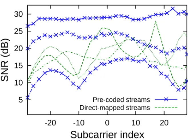
5 10 15 20 25 30
-20 -10 0 10 20
SNR (dB)
Subcarrier index
Pre-coded streams Direct-mapped streamsFigure 5: Precoded vs direct-mapped multiplexing for an example 3x3 testbed link. Precoding deliv-ers more power to the receiver but also results in streams with asymmetric capacity. To use the link optimally, we must also assign power, modulation, and coding differently per stream.
as with line-of-sight links for which multiple antennas often see the same dominant signal. In such cases, it is better to direct a larger fraction of the overall power to the high capacity paths and a smaller fraction of power to the low capacity ones.
A well-known algorithm calledwater-filling [9] maximizes the throughput of multi-stream systems. The key idea is that, because capacity only grows logarithmically with SNR, power allocated to a particular spatial stream will yield di-minishing returns. It is thus inefficient to put all the power into the strongest spatial stream, rather better to balance it among the different spatial streams weighted to optimize the total throughput. The water-filling algorithm gives the transmit power allocations for a particular wireless channel that maximize capacity as a function of the capacity of the individual streams. Of course, to make effective use of the different SNR levels on different spatial streams we must modulate and code individual streams as appropriate.
To see the difference between direct-mapped and precoded multiplexing, we examine another 5.2 GHz link in our 802.11n testbed. For both direct-mapped and precoded MIMO re-ceivers, Figure 5 shows the resulting subcarrier distribution of per-stream SNRs. Direct-mapped MIMO yields three streams with roughly equal performance. In contrast, the three precoded streams have widely varying power levels, indicating asymmetric singular values that reflect correlated spatial paths. The precoded MIMO streams compensate for this situation by putting most of the transmit power into the best two paths, at the expense of weakening the third. The much greater sum SNR for precoded MIMO over direct-mapped MIMO suggests that precoding improves the overall situation, and that by using water-filling to allocate power (and rate) the capacity is increased.
As described above, taking advantage of precoded MIMO requires us to choose modulation and coding rates sepa-rately for each spatial stream. However, 802.11n is designed for implementation on commodity hardware and thus con-strains these choices for multi-stream systems. It provides
some transmit configurations with unequal modulation, but requires a uniform coding rate across streams. Addition-ally, the transmission of multiple signals with wildly different power levels (for the example link,≈20 dB or 100×on some subcarriers) requires a more accurate, hence more expen-sive, power amplifier to maintain signal fidelity; amplifiers are some of the more costly components and manufacturers may in practice opt for cheaper but less accurate designs. These factors will likely limit the extent to which precoded MIMO channels can be optimized in practice, implying a compromise between the solution provided by water-filling and the constraints of the hardware NIC and the available 802.11n rates. Precoded MIMO has the potential to improve performance over direct-mapped MIMO, but it is not widely used in 802.11n NICs yet to the best of our knowledge due to its added complexity.
5.
FURTHER READING
MIMO technologies are rapidly being adopted in 802.11 and other wireless systems, despite their complexity over SISO systems, because of the significant benefits they can deliver in practice. The techniques we described in this tu-torial are the tip of the iceberg. Multiple antennas can also be used for combinations of diversity and multiplexing rather than one or the other. For example, a 3x3 MIMO system might send one, two or three signals, with the extra antennas used for diversity benefits. There is a fundamental tradeoff between the performance from using diversity and multiplex-ing, and the optimal combination depends on the particular MIMO wireless channel and the performance goals [9].
Other advanced topics include multi-user MIMO, in which a node with multiple antennas communicates with multiple users simultaneously to improve performance, and space-time coding, in which information is coded across multiple antennas as well as time. For more information, we refer the interested reader to deeper introductory text [6], textbooks on wireless communications and MIMO [3, 5, 8], and the references therein.
6.
REFERENCES
[1] IEEE Std. 802.11n-2009: Enhancements for higher
throughput.http://www.ieee802.org, 2009.
[2] G. J. Foschini and M. J. Gans. On limits of wireless communications in a fading environment when using
multiple antennas.Wireless Personal Communications,
6:311–335, 1998.
[3] A. Goldsmith.Wireless Communications. Cambridge
University Press, 2005.
[4] G. Judd, X. Wang, and P. Steenkiste. Efficient channel-aware
rate adaptation in dynamic environments. InACM MobiSys,
pages 118–131, 2008.
[5] C. Oestges and B. Clerckx.MIMO Wireless
Communications: From Real-World Propagation to Space-Time Code Design. Academic Press, 2007.
[6] Y. Palaskas, A. Ravi, S. Pellerano, and S. Sandhu. Design Consideration for Integrated MIMO Radio Transceivers. In
K. Iniewski, editor,Wireless Technologies: Circuits,
Systems, and Devices, chapter 4. Taylor & Francis, Inc, 2007. [7] E. Telatar. Capacity of multi-antenna Gaussian channels.
European Trans. Telecommunications, 10(6):585–595, 1999.
[8] D. Tse and P. Viswanath.Fundamentals of Wireless
Communication. Cambridge University Press, 2005. [9] L. Zheng and D. Tse. Diversity and multiplexing: a
fundamental tradeoff in multiple-antenna channels.IEEE