Spatial Data Analysis with R-INLA with Some Extensions

January 2015, Volume 63, Issue 20. http://www.jstatsoft.org/

Spatial Data Analysis with

R

-INLA

with Some

Extensions

Science and Technology

Abstract

The integrated nested Laplace approximation (INLA) provides an interesting way of approximating the posterior marginals of a wide range of Bayesian hierarchical models. This approximation is based on conducting a Laplace approximation of certain functions and numerical integration is extensively used to integrate some of the models parameters out.

TheR-INLApackage offers an interface to INLA, providing a suitable framework for data analysis. Although the INLA methodology can deal with a large number of models, only the most relevant have been implemented within R-INLA. However, many other important models are not available forR-INLAyet.

In this paper we show how to fit a number of spatial models withR-INLA, including its interaction with otherRpackages for data analysis. Secondly, we describe a novel method to extend the number of latent models available for the model parameters. Our approach is based on conditioning on one or several model parameters and fit these conditioned models with R-INLA. Then these models are combined using Bayesian model averaging to provide the final approximations to the posterior marginals of the model.

Finally, we show some examples of the application of this technique in spatial statistics. It is worth noting that our approach can be extended to a number of other fields, and not only spatial statistics.

Keywords: INLA, spatial statistics,R.

1. Introduction

Bayesian inference has become very popular in spatial statistics in recent years. Part of this success is due to the availability of computation methods to tackle fitting of spatial models. Besag, York, and Molli´e(1991) proposed in their seminal paper an appropriate way of fitting

a spatial model using Markov chain Monte Carlo methods. This model has been extensively used and extended to consider different types of fixed and random effects for spatial and spatio-temporal analysis.

In general, fitting these models has been possible because of the availability of different com-putational techniques, the most notable being Markov chain Monte Carlo (MCMC). For large models or big data sets, MCMC can be tedious and reaching the required number of samples can take a long time. Not to mention that autocorrelation may arise and that an increased number of iterations may be required.

Alternatively, the posterior distributions of the parameters may be approximated in some way. However, most models are highly multivariate and approximating the full posterior distribution may not be possible in practice. The integrated nested Laplace approximation (INLA,Rue, Martino, and Chopin 2009) focuses on the posterior marginals for latent Gaussian models. Although these models may seem rather restricted, they appear in a fair number of fields. This also means that INLA will be particularly useful when only marginal inference on the model parameters is needed.

TheR-INLApackage (Rue, Martino, Lindgren, Simpson, Riebler, and Krainski 2014;Lindgren and Rue 2015) for theRprogramming language (RCore Team 2014) provides an interface to INLA (a free-standing programme) so that models can be fitted using standardRcommands. Results are readily available for plotting or further analysis. First of all, we describe how

R-INLAcan be used together with other Rpackages for spatial data analysis. It is often the case that spatial data are available in different formats that need to be loaded into R and some pre-processing is required. Also, once the results are available, it is helpful to explain how to display them on a map.

Although INLA is a general method to approximate the posterior marginals,R-INLA imple-ments a number of popular latent models and prior distributions for the model parameters. It is, however, difficult to fit new models with INLA if these are based on other distributions not available in R-INLA. This may be an inconvenience when trying to develop new models as there is no easy way of extending R-INLA to fit other models without writing them into INLA itself.

This is why we also describe a way of extending the number of models that R-INLA can fit with little extra effort. First of all, we consider one (or more) parameters in our model so that, if they are fixed, the resulting model can be fitted with R-INLA. What we are doing here is, in fact, to fit a model conditioned on the assigned values to the parameters. Then, we can assign different values to these parameters and combine the resulting models in some way to obtain a fit of the original model. We have used Bayesian model averaging and numerical integration techniques to combine these models (Bivand, G´omez-Rubio, and Rue 2014b). This paper is organized as follows. Section 2 describes the integrated nested Laplace ap-proximation. In Section 3 the different latent models for spatial statistics are described. We describe how to extend R-INLA to fit new models in Section4. Some examples are provided in Section 5. Finally, we discuss why our approach is relevant in Section6.

2. Integrated nested Laplace approximation

Bayesian inference is based on computing the posterior distribution of a vector of model parameters x conditioned on the vector of observed data y. Bayes’ rule states that this

posterior distribution can be written down as

π(x|y)∝π(y|x)π(x) (1)

Here,π(y|x) is the likelihood of the model and π(x) represents the prior distribution on the model parameters.

Usually, π(x|y) is a highly multivariate distribution and difficult to obtain. In particular, it is seldom possible to derive it in a closed form. For this reason, several computational approaches have been proposed to get approximations to it. MCMC is probably the most widely used family of computational approaches to estimate the posterior distribution. The marginal distribution of parameter xi can be denoted by π(xi|y) and it can be easily derived from the full posterior by integrating out over the remaining set of parametersx−i. Let us assume that we have a set ofnobservations y={yi}ni=1, whose distribution is of the

exponential family. The mean of observation iis µi and it can depend on a linear predictor

ηi via a link function. In turn, the linear predictor ηi can be modelled as follows:

ηi =α+ nf X j=1 f(j)(uji) + nβ X k=1 βkzki+εi (2)

α is the intercept, f(j) are functions on a set of nf random effects on a vector of covariates

u,βk are coefficients on some covariateszand εi are error terms. Hence, the vector of latent effects is x = {{ηi}, α,{βk}, . . .}. Note that given our particular interest in spatial models, termsf(j)(uji) can be defined as to model spatial or spatio-temporal dependence.

xis modelled using a Gaussian distribution with zero mean and variance-covariance matrix

Q(θ1). Now,θ1 is a vector of hyperparameters. Furthermore, xis assumed to be a Gaussian

Markov random field (GMRF,Rue and Held 2005). This means thatQ(θ1) will fulfil a number

of Markov properties.

The distribution of observationsyi will depend on the latent effectsxand, possibly, a number of hyperparameters θ2. Taking the vector of hyperparameters θ = (θ1, θ2), observations yi will be independent of each other givenxi and θbecause ofx being a GMRF.

Following Rue et al. (2009), the posterior distribution of the model latent effects x and hyperparametersθcan be written as

π(x, θ|y)∝π(θ)π(x|θ)Y i∈I π(yi|xi, θ)∝ (3) π(θ)|Q(θ)|1/2_exp{−1 2x T_Q(θ)x+X i∈I log(π(yi|xi, θ))}

I represents an index of observed data (from 1 to n), Q(θ) is a precision matrix on some hyperparameters θand log(π(yi|xi, θ)) is the log-likelihood of observationyi.

INLA allows different forms for the likelihood of the observations. This includes not only distributions from the exponential family but also mixtures of distributions. Also, INLA can handle observations with different likelihoods in the same model. Regarding the latent effects

x, different models can be used. We will describe some of these in more detail in Section 3. The specification of the prior distributions π(θ) is also very flexible. These will often depend on the latent effect but, in principle, the most common distributions are available and the

user can define their own prior distribution in theR-INLA package (but we will return to this later).

Hence, we can write the marginals of the elements inx and θ (i.e., latent effects and hyper-parameters) as π(xi|y) = Z π(xi|θ,y)π(θ|y)dθ (4) and π(θj|y) = Z π(θ|y)dθ−j (5)

In order to estimate the previous marginals, we need π(θ|y) or, alternatively, a convenient approximation that we will denote by ˜π(θ|y). Initially, this approximation can be taken as

˜ π(θ|y)∝ π(x, θ,y) ˜ πG(x|θ,y) x=x∗_(θ) (6)

Here ˜πG(x|θ,y) is a Gaussian approximation to the full conditional ofxandx∗(θ) is the mode of the full conditional for a given value of θ. Rue et al. (2009) take this approximation and use it to compute the marginal distribution of xi using numerical integration:

˜ π(xi|y) = X k ˜ π(xi|θk,y)×π˜(θk|y)×∆k (7)

Here ∆k are the weights associated with the ensemble of valuesθk, defined on a multidimen-tional grid over the space of hyperparameters.

Note that in the previous equation it is important to have good approximations ofπ(xi|θk,y). A Gaussian approximation ˜πG(xi|θk,y), with meanµi(θ) and variance σi2(θ), may be a good starting point but a better approximation may be required in other cases. Rue et al. (2009) developed better approximations based on alternative approximation methods, such as the Laplace approximation. For example, they have used the Laplace approximation to obtain:

˜ πLA(xi|θ,y)∝ π(x, θ,y) ˜ πGG(x−i|xi, θ,y) x−i=x∗−i(xi,θ) (8) ˜

πGG(x−i|xi, θ,y) is a Gaussian approximation to x−i|xi, θ,y around its modex∗−i(xi, θ). Rue et al. (2009) develop a simplified Laplace approximation to improve ˜πLA(xi|θ,y) using a series expansion of the Laplace approximation around xi. This approximation is computa-tionally less expensive, and it also corrects for location and skewness.

2.1. The R-INLA package

An interface to INLA has been provided as an R package called R-INLA, which can be downloaded from http://www.r-inla.org/, together with the free-standing external INLA programme. R-INLAprovides a user model interface similar to the one used to fit generalized additive models (GAM) with functiongam()in themgcvpackage (Wood 2006). It can handle fixed effects, non-linear terms and random effects in a formula argument. The interface is flexible enough to allow for the specification of different priors and model fitting options. Non-linear terms and random effects are included in the formula as calls to the f()function.

The model is fitted with a call to function inla(), which will return the fitted model as an inla object. Note that, by default, only some results will be returned. These include the marginal distributions of the latent effects and hyperparameters, as well as summary statistics.

In addition to the posterior marginals,R-INLAcan provide a number of additional quantities on the fitted model. For example, it can provide the log-marginal likelihoodπ(y) which can be used for model selection. Other model selection criteria such as the DIC (Spiegelhalter, Best, Carlin, and Van der Linde 2002) and CPO (Held, Sch¨odle, and Rue 2010) have also been implemented.

Furthermore, R-INLA includes a number of options to define the prior distributions for the parameters in the model. Well-known prior distributions are available and the user can define their own prior distributions as well.

In the next Section we describe different examples of the use of R-INLA for spatial statistics, in which we have included a detailed description on howinla() should be called.

3. Spatial models with INLA

As discussed in Section2, spatial dependence can be included as part of the vector of latent effects x. In principle, any number of random effects can be included in the model. In this Section, we will describe the different options available, depending on the type of problem. A full description of the models described here can be found in the R-INLA website at http: //www.r-inla.org/, but we have included a summary. Blangiardo, Cameletti, Baio, and Rue (2013) and G´omez-Rubio, Bivand, and Rue (2014b) also discuss the different spatial models included inR-INLA.

First we will briefly introduce other papers describing the use of INLA andR-INLAfor spatial statistics. Schr¨odle and Held(2010) describe the use of spatial and spatio-temporal models for disease mapping, including ecological regression. Schr¨odle and Held(2011) expand the number of spatio-temporal models that can be used withR-INLA, and show the use of setting linear constraints to make complex spatio-temporal effects identifiable. Schr¨odle, Held, Riebler, and Danuser (2011) show how to use spatio-temporal models for disease surveillance. Eidsvik, Finley, Banerjee, and Rue(2012) focus on the use of R-INLA for the analysis of large spatial datasets. Finally,Ruiz-Cardenas, Krainski, and Rue(2012) develop spatio-temporal dynamic models withR-INLA.

3.1. Analysis of lattice data

First of all, we will discuss the analysis of lattice data because this will establish the basis for other types of analyses. In the analysis of lattice data observations are grouped according to a set of areas, which usually represent some sort of administrative region (neighborhoods, municipalities, provinces, countries, etc.).

R-INLA includes a latent model for uncorrelated random effects. In this case, the random effectsui are modelled as

ui ∼N(0, τu) (9)

whereτu refers to the precision of the Gaussian distribution. It should be noted thatR-INLA assigns a prior to log(τu) which, by default, is a log-gamma distribution. Although this model

is not spatial, it can be combined with other spatial models. Using log(τu) instead of simply

τu provides some advantages as log(τu) is not constrained to be positive. This is particularly useful when optimising to find the mode of log(τu), for example.

In order to model spatial correlation, neighborhoods must be defined among the study areas. It is often considered that two areas are neighbors is they share a common boundary. Spatial autocorrelation is modelled using a Gaussian distribution with zero mean and a precision matrix that will model correlation between neighbors. Given that latent effects are a GMRF, we can define the variance-covariance matrix of the random effects as

Σ = 1

τQ

−1 ₍₁₀₎

whereτ is a precision parameter and matrix Qencodes the spatial structure. Given that we are assuming a latent GMRF, this also means that matrixQwill be defined such as element

Qij is zero if areasiandjare not neighbors. This means thatQis often a very sparse matrix. See, for example,Rue and Held(2005) for details.

Available specifications for spatial dependence includes the intrinsic conditional autoregressive (CAR) specification (Besaget al.1991). This will produce a Qmatrix in which element Qii isni (the number of neighbors of area i) and element Qij (with i6=j) is -1 if areasi and j are neighbors and 0 otherwise. This means that the spatial random effectsvi are distributed as vi|vj, τv ∼N( 1 ni X i∼j vj, 1 τvni ) i6=j (11)

τv is the conditional precision of the random effects. As in the previous model, R-INLA uses a log-gamma prior on log(τv).

In addition, a proper version of this model is available as well, for which the spatial random effects are distributed as

vi|vj, τv ∼N( 1 ni+d X i∼j vj, 1 τv(ni+d) ) i6=j (12)

dis a positive quantity to make the distribution proper. By default, a log-gamma distribution is assigned to log(d).

A more general approach is obtained with the following precision matrix:

Q= (I − ρ

λmax

C) (13)

Here I is the identity matrix, ρ a spatial autocorrelation parameter, C an adjacency matrix and λmax the maximum eigenvalue ofC. R-INLAassigns a Gaussian prior on log(ρ/(1−ρ)). This specification ensures that ρ takes values between 0 and 1.

In the following example we use the Boston housing data, which is described in Harrison and Rubinfeld(1978), to develop an example on several spatial models. This data set records median price for houses that were occupied by their owners plus some other relevant covariates (seeHarrison and Rubinfeld 1978;Pace and Gilley 1997, for details). Data have been recorded at the tract level and the neighborhood structure of the tracts is also available, and it is available in the boston data set from the Rpackage spdep(Bivand 2014). In addition, this data set is also available in a shapefile, which is the one we will use in this example. This

will provide a more general example on how to load external data intoR to fit models with

R-INLA.

readShapePoly(), from packagemaptools(Bivand and Lewin-Koh 2014), can be used to load vector data from a shapefile. Alternatively, readOGR(), from package rgdal (Bivand, Keitt, and Rowlingson 2014a), provides a more general data loading framework for vector data since it supports a wider range of formats. This is the one we have used to load the Boston data set:

R> library("rgdal")

R> boston <- readOGR(system.file("etc/shapes", package = "spdep")[1], + "boston_tracts")

Here,readOGR()takes the directory where the layer (shapefile) is located and the layer name, which in this case is the name of the shapefile, as arguments and return an object of type SpatialPolygonsDataFrame. This data object is used to store the tract boundaries plus the associated data (tract name and other variables).

Before fitting any spatial model, the neighborhood structure needs to be defined. A common criterion is to consider that two areas are neighbors if they share a common boundary. Func-tionpoly2nb()will take the tract boundaries and perform this operation to provide us with the adjacency structure of the Boston tracts as anb object:

R> library("spdep")

R> bostonadj <- poly2nb(boston, queen = FALSE)

Here, we have also set queen = FALSE so that queen adjacency is not used, i.e., in order to consider two areas as neighbors more than one shared point is required. We have converted this into a binary matrix to be used with R-INLA using function nb2mat(). Furthermore, the adjacency matrix is converted into a sparse matrix of classdgTMatrixto reduce memory usage. This will be passed to functionf()when defining the spatial model.

R> adj <- nb2mat(bostonadj, style = "B") R> adj <- as(adj, "dgTMatrix")

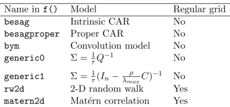
A summary of some latent models implemented in R-INLA, and that can be used within thef() function, is available in Table 1. Note that this is not an exhaustive list and that a complete list of the available latent models can be obtained from theR-INLAdocumentation. We have also included a column showing whether these models are restricted to a regular grid. Also, detailed examples are available from theR-INLAwebsite athttp://www.r-inla.org/. Fixed effects (including the intercept) inR-INLA have a Gaussian prior with fixed mean and precision, which are 0 and 0.01 (or 0 for the intercept) by default, respectively. These values can be changed using optioncontrol.fixed in the inla() call. control.fixed must take a named list of arguments, which are used to control how to handle the fixed effects in the model.

In this named list,mean.intercept andprec.intercept can be used to set the parameters of the Gaussian prior of the intercept, whilstmeanand precare the analogous parameters to define the priors for the other fixed effects. These can be a numeric value or another named list, using the names of fixed effects, to set different priors for different effects. Note that

Name in f() Model Regular grid

besag Intrinsic CAR No

besagproper Proper CAR No

bym Convolution model No

generic0 Σ = 1_τQ−1 No

generic1 Σ = 1_τ(In− _λmaxρ C)−1 No

rw2d 2-D random walk Yes

matern2d Mat´ern correlation Yes

Table 1: Summary of some latent models implemented inR-INLA for spatial statistics.

precisions in the fixed effects priors cannot be estimated as was the case with the different random effects presented before.

The model that we are fitting is:

yi =α+βXi+vi+εi (14)

where α is the model intercept, β a vector of coefficients of the covariates Xi, vi a random effect with an intrinsic CAR specification andεi is random Gaussian error term.

Asf() needs an area index which must have different values for different areas, this is first defined in variableidx.

R> library("INLA")

R> boston$idx <- 1:nrow(boston)

R> form <- log(CMEDV) ~ CRIM + ZN + INDUS + CHAS + I(NOX^2) + I(RM^2) +

+ AGE + log(DIS) + log(RAD) + TAX + PTRATIO + B + log(LSTAT) +

+ f(idx, model = "besag", graph = adj) R> btdf <- as.data.frame(boston)

R> m1 <- inla(form, data = btdf, control.predictor = list(compute = TRUE))

Note how the call toinla() is similar to fitting other regression models with Rwith glm() or gam(). Furthermore, it is very easy to include spatial random effects with function f() in theformulapassed toinla(). Finally,control.predictor = list(compute = TRUE)is used to compute summary statistics on the fitted values.

A summary of the model can be obtained as follows:

R> summary(m1)

Call:

"inla(formula = form, data = btdf, control.predictor = list(compute = TRUE))" Time used:

Pre-processing Running inla Post-processing Total

0.5940 2.2684 0.1178 2.9802

mean sd 0.025quant 0.5quant 0.975quant mode kld (Intercept) 3.7798 0.1661 3.4536 3.7798 4.1058 3.7798 0 CRIM -0.0073 0.0011 -0.0094 -0.0073 -0.0053 -0.0073 0 ZN 0.0003 0.0005 -0.0006 0.0003 0.0013 0.0003 0 INDUS -0.0005 0.0024 -0.0051 -0.0005 0.0041 -0.0005 0 CHAS1 -0.0443 0.0299 -0.1030 -0.0443 0.0144 -0.0443 0 I(NOX^2) -0.4209 0.1440 -0.7037 -0.4210 -0.1384 -0.4209 0 I(RM^2) 0.0101 0.0011 0.0080 0.0101 0.0122 0.0101 0 AGE -0.0012 0.0005 -0.0022 -0.0012 -0.0003 -0.0012 0 log(DIS) -0.1806 0.0719 -0.3217 -0.1806 -0.0395 -0.1806 0 log(RAD) 0.0483 0.0208 0.0076 0.0483 0.0891 0.0483 0 TAX -0.0003 0.0001 -0.0005 -0.0003 0.0000 -0.0003 0 PTRATIO -0.0162 0.0053 -0.0265 -0.0162 -0.0058 -0.0162 0 B 0.0006 0.0001 0.0003 0.0006 0.0008 0.0006 0 log(LSTAT) -0.2434 0.0223 -0.2873 -0.2434 -0.1996 -0.2434 0 Random effects: Name Model

idx Besags ICAR model Model hyperparameters:

mean sd

Precision for the Gaussian observations 1.626e+04 1.707e+04

Precision for idx 1.222e+01 7.817e-01

0.025quant 0.5quant Precision for the Gaussian observations 7.582e+02 1.096e+04

Precision for idx 1.074e+01 1.220e+01

0.975quant mode Precision for the Gaussian observations 6.180e+04 1.816e+03

Precision for idx 1.381e+01 1.216e+01

Expected number of effective parameters(std dev): 501.85(5.348) Number of equivalent replicates : 1.008

Marginal Likelihood: -212.85

Posterior marginals for linear predictor and fitted values computed

The output includes summary statistics of the posterior marginals of the coefficients of the fixed effects plus the precisions of the error term and intrinsic CAR random effect. In addi-tion,kldreports the Kullback-Leibler divergence between the Gaussian and the (simplified) Laplace approximation to the marginal posterior densities. This provides information about the accuracy of the Gaussian approximation.

The marginal likelihood of the model is also reported and it is computed by integrating all the model parameters out. Hence, it is not thepredictive marginal likelihood and it can be used to perform model selection, for example. The effictive number of parameters, as defined in Spiegelhalteret al.(2002), and the associated number of equivalent replicates are also shown. See Martino and Rue(2010) for more details on the R-INLA output.

3.0 3.5 4.0 4.5 0.0 1.0 2.0 (Intercept) x y −0.012 −0.006 0 200 CRIM x y −0.002 0.000 0.002 0 400 800 ZN x y −0.010 0.000 0.010 0 50 150 INDUS x y −0.15 −0.05 0.05 0 4 8 12 CHAS1 x y −1.0 −0.6 −0.2 0.2 0.0 1.0 2.0 I(NOX^2) x y 0.006 0.010 0.014 0 200 I(RM^2) x y −0.003 −0.001 0.001 0 400 800 AGE x y −0.5 −0.3 −0.1 0.1 0 2 4 log(DIS) x y −0.05 0.05 0.15 0 5 10 20 log(RAD) x y −8e−04 −2e−04 0 1500 3500 TAX x y −0.04 −0.02 0.00 0 20 60 PTRATIO x y 0e+00 6e−04 0 1500 3500 B x y −0.35 −0.25 −0.15 0 5 10 log(LSTAT) x y

0e+00 2e+05 4e+05

0e+00 4e−05 Precision error x y 10 12 14 16 0.0 0.2 0.4

Precision spatial effects

x

y

Figure 1: Marginals of the fixed effects, and the precisions of the error term and spatial random effects, Boston housing data.

Figure1shows the estimated marginals of the coefficients of the fixed effects and the precisions of the random effects in the model. These distributions can be used to compute summary statistics for the model parameters. In the previousR-INLAoutput these marginals have been used to compute the posterior mean, standard deviation, mode and some quantiles (0.025, 0.5 and 0.975).

Fitted values can be easily displayed in a map. First, we need to add all the required values to theSpatialPolygonsDataFrame:

R> boston$LOGCMEDV <- log(boston$CMEDV)

R> boston$FTDLOGCMEDV <- m1$summary.fitted[, "mean"]

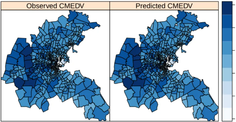
Observed CMEDV Predicted CMEDV 1.5 2.0 2.5 3.0 3.5 4.0

Figure 2: Observed and predicted median values, Boston housing data.

both the observed and the predicted values of house prices. In the following example, which can be seen in Figure2, we have also used packageRColorBrewer(Neuwirth 2014) to define a suitable color palette:

R> library("RColorBrewer")

R> spplot(boston, c("LOGCMEDV", "FTDLOGCMEDV"),

+ col.regions = brewer.pal(9, "Blues"), cuts = 8,

+ names.attr = c("Observed log-CMEDV", "Predicted log-CMEDV"))

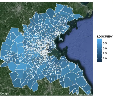
To provide an alternative visualisation of the results, we have included a short example using function qmap() from the ggmap package (Kahle and Wickham 2013). First of all we will reproject our data to be WGS84. With fortify() the boston dataset is converted into a suitable format to be used when plotting and then the log median values are added to the new data.

R> bostonf <- spTransform(boston, CRS("+proj=longlat +datum=WGS84")) R> library("ggmap")

R> bostonf <- fortify(bostonf, region = "TRACT")

R> idx <- match(bostonf$id, as.character(boston$TRACT)) R> bostonf$LOGCMEDV <- boston$LOGCMEDV[idx]

qmap()is based on the the grammar of graphics implemented in the ggplot2package (Wick-ham 2009). In the next example, qmap() is used to get satellite data from the Boston area, whilstgeom_polygon()adds the boundaries:

R> qmap("boston", zoom = 10, maptype = "satellite") + geom_polygon(

+ data = bostonf, aes(x = long, y = lat, group = group, fill = LOGCMEDV),

+ colour = "white", alpha = 0.8, size = 0.3)

Figure 3: Display of the Boston housing data set usingggmapand Google Maps.

3.2. Point patterns

Point patterns are analyzed with INLA as the result of a counting process, i.e., points are not modelled directly but they are aggregated over a a grid of small squares. For this reason, the analysis of point patterns is conducted similarly to that of lattice data: counts are available for each square and these are assigned neighbors according to the adjacent squares. Then, counts can be smoothed using an appropriate non-linear term, such as spatial random effects. Hossain and Lawson(2009) compare different approximations to the analysis of point patterns, including methods that are based on discretisation of the study region.

In the following example we use the Japanese black pine data set from R package spatstat (Baddeley and Turner 2005). This data set records the location of Japanese black pine saplings in a square sampling in a natural forest. This example is reproduced fromG´omez-Rubioet al.

(2014b).

Hence, we first split the study area into smaller squares to create a grid of 10×10 squares.

R> library("spatstat") R> data("japanesepines") R> japd <- as.data.frame(japanesepines) R> Nrow <- 10 R> Ncol <- 10 R> n <- Nrow * Ncol R> grd <- GridTopology(cellcentre.offset = c(0.05, 0.05),

After the creation of the grid, we have used function over() on the set of points and the newly defined squares to find how many points can be found in each square.

R> polygrdjap <- as(grd, "SpatialPolygons")

R> idxpp <- over(SpatialPoints(japd), polygrdjap)

R> japgrd <- SpatialGridDataFrame(grd, data.frame(Ntrees = rep(0, n))) R> tidxpp <- table(idxpp)

R> japgrd$Ntrees[as.numeric(names(tidxpp))] <- tidxpp

Next, an index variable is built to create the spatial neighborhood structure to be passed to the f() function. Note that care must be taken as R and R-INLA may have a different ordering of the areas when defining the adjacency matrix.

R> japgrd$SPIDX <- 1:n

R> japnb <- poly2nb(polygrdjap, queen = FALSE, row.names = 1:100) R> adjpine <- nb2mat(japnb, style = "B")

R> adjpine <- as(adjpine, "dgTMatrix")

Here we have avoided using a queen adjacency as this will consider as neighbors two areas which only share a corner.

Finally, we define the call toinla() using aformula which includes spatial random effects based on the grid of squares. In addition, we have set other options to compute the DIC, with control.compute = list(dic = TRUE), and the marginals of the linear predictors, using control.predictor = list(compute = TRUE). We have included the specification of the prior distributions of the log-precisions of unstructured and spatial random effects as well.

R> fpp <- Ntrees ~ 1 + f(japgrd$SPIDX, model = "bym", graph = adjpine,

+ hyper = list(prec.unstruct = list(prior = "loggamma",

+ param = c(0.001, 0.001)),

+ prec.spatial = list(prior = "loggamma", param = c(0.1, 0.1))))

R> japinlala <- inla(fpp, family = "poisson", data = as.data.frame(japgrd),

+ control.compute = list(dic = TRUE),

+ control.inla = list(tolerance = 1e-20, h = 1e-08),

+ control.predictor = list(compute = TRUE))

R> japgrd$INLALA <- japinlala$summary.fitted.values[, "mean"]

The former model is the one that we have employed with the Boston data set on an irregular lattice. Given that now we are considering a regular lattice it is also possible to use a two-dimensional random walk for spatial smoothing:

R> fpprw2d <- Ntrees ~ 1 + f(japgrd$SPIDX, model = "rw2d", nrow = 10,

+ ncol = 10, hyper = list(prec = list(prior = "loggamma",

+ param = c(0.001, 0.001))))

R> japinlalarw2d <- inla(fpprw2d, family = "poisson",

+ data = as.data.frame(japgrd), control.compute = list(dic = TRUE),

+ control.inla = list(tolerance = 1e-20, h = 1e-08),

+ control.predictor = list(compute = TRUE))

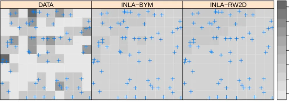
DATA INLA−BYM INLA−RW2D 0.0 0.5 1.0 1.5 2.0 2.5 3.0

Figure 4: Estimation of the intensity of a point pattern with R-INLA, Japanese black pine dataset.

Figure 4 shows the original counts and the smoothed counts. Note that this is similar to estimating the intensity of an inhomogeneous point pattern using a smoothing method. 3.3. Geostatistics

R-INLAdeals with geostatistical data on a regular grid. This means that observations need to be matched to the points in the grid and that those points with no observations attached are considered as missing values. Hence, this is somewhat similar to the analysis of lattice data and point patterns. However, R-INLA provides a number of options to build model-based geostatistical models (Diggle and Ribeiro 2007). First of all, different likelihoods can be used. Secondly, there are different options to define the spatial random effects. Although it is still possible to model spatial dependence in the grid of points using a CAR specification,R-INLA provides a two-dimensional Mat´ern covariance function.

This correlation allows, for example, the use of exponentially decaying functions such as

Σij =σ2exp(−dij/ϕ) (15)

wheredij is the distance between pointsiand j, andϕis a parameter that controls the scale of the spatial dependence.

More recently, Lindgren, Rue, and Lindstr¨om (2011) follow a different approach based on a triangulation on the sampling points and the use of stochastic partial differential equations. Now, the spatial effects are defined as

u(s) =

n

X

k=1

ψk(s)wk, s∈R2 (16)

Here, {ψk(s)} are a basis of functions and wk are associated weights. Weights are assumed to be Gaussian. The advantages of this approach for spatial statistics are fully described in Cameletti, Lindgren, Simpson, and Rue(2013).

In order to show how to fit geostatistical models withR-INLAwe reproduce here an example fromG´omez-Rubioet al.(2014b) based on the Rongelap data set (Diggle and Ribeiro 2007), which records radionuclide concentration at 157 different locations in Rongelap island. We have restricted the analysis to one of the clusters in the north-east part of the island because

observations need to be matched to a regular grid of points. For this analysis we have usedR

packages geoR (Ribeiro and Diggle 2001) and geoRglm(Christensen and Ribeiro 2002). First of all, data are loaded and the data from the desired clusters are extracted from the original data set by checking that their coordinates are in the window (−700,−500)× (−1900,−1700). R> library("geoR") R> library("geoRglm") R> data("rongelap") R> rgldata <- as.data.frame(rongelap) R> xy <- rongelap[[1]]

R> idx1 <- (xy[, 1] < -500 & xy[, 1] > -700 & xy[, 2] > -1900 &

+ xy[, 2] < -1700)

R> rgldata <- rgldata[idx1, ]

The next step is to define the grid topology for the grid that will be used to match these points to. The grid is defined to be of dimension 5×5.

R> Nrow <- 5 R> Ncol <- 5

R> n <- Nrow * Ncol

R> grdoffset <- c(min(rgldata$X1), min(rgldata$X2)) R> csize1 <- diff(range(rgldata$X1))/(Nrow - 1) R> csize2 <- diff(range(rgldata$X2))/(Ncol - 1)

R> grd <- GridTopology(cellcentre.offset = grdoffset,

+ cellsize = c(csize1, csize2), cells.dim = c(Nrow, Ncol))

Data will be placed in aSpatialGridDataFrame(using the previously defined grid topology) and re-organized according to whatR-INLA expects for this model (i.e., grid data stored by column). An index variableIDXis added to be used inf()when defining the model. However,

R-INLA will rely on how the rows are ordered in the data passed to inla() when defining distances and adjacencies (i.e., the index variable ordering will not be considered).

R> inla2sp <- inla.lattice2node.mapping(Nrow, Ncol)[, Ncol:1] R> inla2sp <- as.vector(inla2sp)

R> spgrd <- SpatialGridDataFrame(grd, as.data.frame(rgldata[inla2sp, ])) R> spgrd$IDX <- 1:nrow(spgrd@data)

Next, we create aSpatialPolygonswith the boundaries of the squares in the grid. This way, it is easy to match the data to the newly created grid using functionover().

R> polygrd <- as(grd, "SpatialPolygons")

R> dataidx <- over(SpatialPoints(as.matrix(rgldata[, 1:2])), polygrd)

It should be noted that radionuclide concentration is measured at each square by the average of the observations in the square, and this needs to be computed beforehand.

R> yag <- by(rgldata$data, dataidx, sum) R> umag <- by(rgldata$units.m, dataidx, sum) R> ratioag <- yag/umag

DATA INLA−MATERN2D INLA−RW2D 0 2 4 6 8 10 12

Figure 5: Observed and estimated radionuclide concentration in Rongelap island.

Then, a new column is added to the SpatialGridDataFramewith these averages. NAwill be used for the squares with no data so that these values will be imputed from the model.

R> spgrd$ratioag <- NA

R> spgrd$ratioag[as.numeric(names(ratioag))] <- ratioag

Here we define a model with an intercept term and a random effect of the Mat´ern class. Note how we have fixed, for convenience, the value of the range and precision.

R> formula1 <- ratioag ~ 1 + f(spgrd$IDX, model = "matern2d", nrow = Nrow,

+ ncol = Ncol, hyper = list(range = list(initial = log(sqrt(8)/0.5),

+ fixed = TRUE), prec = list(initial = log(1), fixed = TRUE)))

R> rglinlala <- inla(formula1, family = "poisson",

+ control.predictor = list(compute = TRUE),

+ control.compute = list(dic = TRUE),

+ data = as.data.frame(spgrd))

R> spgrd$INLALA <- rglinlala$summary.fitted.values[, "mean"]

Similarly as in the point patterns example, here we have also used a two dimensional random walk for spatial smoothing.

R> formularw2d <- ratioag ~ 1 + f(spgrd$IDX, model = "rw2d", nrow = Nrow,

+ ncol = Ncol, hyper = list(prec = list(prior = "loggamma",

+ param = c(1, 1))))

R> rglinlalarw2d <- inla(formularw2d, family = "poisson",

+ control.predictor = list(compute = TRUE),

+ control.compute = list(dic = TRUE),

+ data = as.data.frame(spgrd))

R> spgrd$INLALARW2D <- rglinlalarw2d$summary.fitted.values[, "mean"]

Figure5shows the observed and estimated radionuclide concentration in Rongelap island. It can be seen how our model has spatially smoothed the observed values.

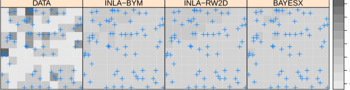
DATA INLA−BYM INLA−RW2D BAYESX 0.0 0.5 1.0 1.5 2.0 2.5 3.0

Figure 6: Estimation of the intensity of a point pattern withR-INLA andBayesX, Japanese black pine dataset.

3.4. R-INLA and other packages for Bayesian spatial modelling

R-INLAis not the only package for Bayesian spatial modelling. Bivand, Pebesma, and G´ omez-Rubio (2013, Chapter 10) compare different packages for Bayesian modelling in the contect of disease mapping. We wil focus here in R2BayesX(Umlauf, Kneib, Lang, and Zeileis 2013; Umlauf, Adler, Kneib, Lang, and Zeileis 2015) because it provides a way to defining spatial models as R-INLA.

For example, in order to reproduce the example on the Japanese black pine data with R2BayesX we can do the following:

R> library("R2BayesX")

R> bayesxadj <- nb2gra(japnb)

R> japbyx <- bayesx(Ntrees ~ 1 + sx(SPIDX, bs = "re") +

+ sx(SPIDX, bs = "spatial", map = bayesxadj), family = "poisson",

+ data = as.data.frame(japgrd))

Functionnb2gra()is used to convert our adjacency matrix into an object of classgra, which is used in R2BayesXto store adjacencies. bayesx()takes similar arguments asinla()and the model can be expressed using aformula, withsx()used to define the random effects. sx(idx, bs = "re") defines independent Gaussian random effects and the spatial random effects are defined insx(TRACT, bs = "spatial", map = bayesxadj)using adjancency matrix defined in bayesxadj.

Retrieving the predicted data requires some care as they are reordered, but is is as simple as:

R> japgrd$BAYESX <- japbyx$fitted.values[ + order(japbyx$bayesx.setup$order), "mu"]

Finally, we compare the fitted values obtained withR-INLAandR2BayesXin Figure6. Note that differences appear not only because of the different models used but also because of the choice of prior distributions.

4. Extending

R

-

INLA

to fit new models

Although the current implementation of INLA in theR-INLA package provides a reasonable number of models for spatial dependence it may be the case that we need to include some other models. As it is now, this is not possible without adding to the code of the external INLA programme.

Bivandet al.(2014b) describe a simple way of extending INLA to use other latent models. In particular they focus on some latent models used in spatial econometrics that are not available as part of the R-INLA package at the moment. A new latent class has been added recently and it is described in G´omez-Rubio, Bivand, and Rue (2014a).

This approach is based on considering a model where one or several parameters have been fixed in a way that makes the conditioned model fittable withR-INLA. If we denote byρthe vector of parameters to fix and by ˆρ a specific set of fixed parameter values, the full posterior marginal could be written as

π(x, θ|y,ρˆ) (17)

Taking this into account, it is clear that when conditioning on ρ= ˆρ R-INLA will give us an approximation to π(xi|y,ρˆ) andπ(θi|y,ρˆ).

Note that the full posterior distribution can be obtained by integrating ρ out, i.e.,

π(x, θ|y) =

Z

π(x, θ|y, ρ)π(ρ|y)dρ (18)

where π(ρ|y) is the posterior distribution of ρ. Also, note that this can be written as

π(ρ|y)∝π(y|ρ)π(ρ) (19)

Here π(ρ) is a prior distribution on ρ and π(y|ρ) is the marginal likelihood of the model, which is reported by R-INLA. Hence,π(ρ|y) can be estimated by re-scaling the expression in Equation19.

The posterior distribution ofρcan be estimated by defining a fine grid of values S ={ρi}r_i=1 so that π(ρi|y), i = 1, . . . , r are computed. Then π(ρ|y) can be obtained by fitting and re-scaling a spline (or other non-linear function) to the previous values. Using simple numerical integration techniques we can obtain an approximation to π(x, θ|y) as follows:

π(x, θ|y) =

Z

π(x, θ|y, ρ)π(ρ|y)dρ' X

ρi∈S

π(x, θ|y, ρi)π(ρi|y)∆i (20)

where ∆i is the amplitude of the interval used in the discretisation of ρ.

Note that the previous expression can be regarded as a weighted average of the different models fitted after conditioning on different values of ρ.

From Equation 20it is clear that we can obtain the following approximations to the posterior marginals of the individual latent parameters and hyperparameters:

ˆ π(xi|y) = X j π(xi|y, ρj)wj (21) ˆ π(θi|y) = X j π(θi|y, ρj)wj (22)

wj is a weight associated with ρj as follows:

wj =π(ρj|y)∆j (23)

This is like carrying out Bayesian model averaging (Hoeting, Madigan, Raftery, and Volinsky 1999) on the different conditioned models fitted withR-INLA. Altogether, this provides a way of combining simpler models to obtain our desired model. In Section5we show how to apply these ideas to different models in spatial statistics.

Note that this approach can be easily extended to the case of ρ being a discrete random variable.

4.1. Implementation

We have implemented this approach in anRpackage calledINLABMA, available from CRAN. The package includes some general functions to conduct Bayesian model averaging of models fitted with INLA. In addition, we have included some wrapper functions to fit the models described in Section5.

5. Examples

5.1. Leroux model

Leroux, Lei, and Breslow(1999) propose a model for the analysis of spatial data in a lattice which is similar to the one by Besag et al. (1991), in the sense that they split variation according to spatial and spatial patterns. Rather than including the spatial and non-spatial random effect as a sum in the linear term they consider a single random effect as follows:

u∼MVN(0,Σ); Σ =σ2((1−λ)In+λM)−1 (24) Here M is the precision matrix of a process with spatial structure and we will take that of an intrinsic CAR specification. Hence, the precision matrix is, in a sense, a mixture of the precisions of a non-spatial and a spatial one. λ controls how strong the spatial structure is. Forλ= 1 the effect is entirely spatial whilst for λ= 0 there is no spatial dependence. In principle, this is not a model thatR-INLAcan fit. However, if λis fixed, then the random effects are Gaussian with a known structure for the variance-covariance matrix which can be fitted using ageneric0 latent model.

Boston housing data

Here we revisit the Boston housing data to fit the Leroux et al. model. First of all, it is worth mentioning that the model needs a wrapper function to be fitted for a given value of the spatial parameterλ. This wrapper function is included in the Rpackage R-INLA and it is based on thegeneric0latent model available inR-INLA. Onceλis fixed the model can be easily fitted withR-INLA, as the latent effect is a multivariate Gaussian random effect with zero mean and precision matrix as in Equation 24. We repeat this procedure for different values ofλto obtain a list of fitted models to be combined later.

Hence, we have written a simple wrapper function which is included in packageINLABMA (G´omez-Rubio and Bivand 2014):

R> library("INLABMA") R> leroux.inla

function (formula, d, W, lambda, improve = TRUE, fhyper = NULL, ...) {

W2 <- diag(apply(W, 1, sum)) - W

Q <- (1 - lambda) * diag(nrow(W)) + lambda * W2 assign("Q", Q, environment(formula))

if (is.null(fhyper)) {

formula <- update(formula, . ~ . + f(idx, model = "generic0", Cmatrix = Q))

} else {

formula <- update(formula, . ~ . + f(idx, model = "generic0", Cmatrix = Q, hyper = fhyper))

}

res <- INLA::inla(formula, data = d, ...) if (improve)

res <- INLA::inla.rerun(res)

res$logdet <- as.numeric(Matrix::determinant(Q)$modulus) res$mlik <- res$mlik + res$logdet/2

return(res) }

<environment: namespace:INLABMA>

In the previous code, the precision matrixQis created using the adjacency matrixWand the value of λ. Then thegeneric0model is added to the formula with the fixed effects. Finally we correct the marginal log-likelihood π(y|λ) (conditioned on the value ofλ) by adding half the log-determinant of ((1−λ)In+λM). Note that, in principle, this is not needed to fit a single model and obtain the approximations to the posterior marginals as it is a constant. However, we are fitting and combining several models so we need to correct for this because this scaling factor will change with the value of λ. Argument ... is used to pass any other options to inla(). This can be used to tune and set a number of other options.

Also, the adjacency matrix is taken from the data provided in the boston data set. Note that we will be using a binary adjacency matrix as the random effects have an intrinsic CAR specification:

R> boston.matB <- listw2mat(nb2listw(bostonadj, style = "B")) R> bmspB <- as(boston.matB, "CsparseMatrix")

Function inla.leroux is used in the example below to compute the fitted models for the Leroux et al. model. In this case, we take λ to be in the interval (0.8,0.99) after previous assessment on where π(λ|y) has its mode. Also, we define a prior for the precision of the random effects in variable fhyper. The prior for the precision of the error term is defined in errorhyper. In addition, we have usedmclapplyto parallelize the computations on operating systems supporting forking (not Windows). Note that this is an advantage of fitting these conditioned models compared with standard MCMC methods.

Mean (INLA) SD (INLA) Mean (MCMC) SD (MCMC) Intercept 3.8055 0.1770 3.8018 0.1651 CRIM −0.0076 0.0011 −0.0077 0.0011 ZN 0.0003 0.0005 0.0003 0.0004 INDUS −0.0006 0.0023 −0.0007 0.0023 CHAS1 −0.0338 0.0302 −0.0342 0.0305 I(NOX^2) −0.4374 0.1412 −0.4467 0.1380 I(RM^2) 0.0099 0.0011 0.0099 0.0011 AGE −0.0011 0.0005 −0.0011 0.0005 log(DIS) −0.1663 0.0616 −0.1624 0.0618 log(RAD) 0.0506 0.0205 0.0484 0.0220 TAX −0.0003 0.0001 −0.0003 0.0001 PTRATIO −0.0164 0.0053 −0.0164 0.0053 B 0.0006 0.0001 0.0006 0.0001 log(LSTAT) −0.2534 0.0227 −0.2521 0.0221 λ 0.9520 0.0315 0.9401 0.0342

Table 2: Point estimates of fixed effects andλusing INLA and MCMC.

R> rlambda <- seq(0.8, 0.99, length.out = 20)

R> fhyper <- list(prec = list(prior = "loggamma", param = c(0.001, 0.001),

+ initial = log(1), fixed = FALSE))

R> errorhyper <- list(prec = list(prior = "loggamma",

+ param = c(0.001, 0.001), initial = log(1), fixed = FALSE))

R> form2 <- log(CMEDV) ~ CRIM + ZN + INDUS + CHAS + I(NOX^2) + I(RM^2) +

+ AGE + log(DIS) + log(RAD) + TAX + PTRATIO + B + log(LSTAT)

R> lerouxmodels <- mclapply(rlambda, function(lambda) {

+ leroux.inla(form2, d = as.data.frame(boston), W = bmspB,

+ lambda = lambda, fhyper = fhyper, improve = TRUE,

+ family = "gaussian", control.fixed = list(prec.intercept = 0.001,

+ prec = 0.001), control.family = list(hyper = errorhyper),

+ control.predictor = list(compute = TRUE),

+ control.compute = list(dic = TRUE, cpo = TRUE),

+ control.inla = list(print.joint.hyper = TRUE))

+ })

Following this, we need to combine the different models to obtain the final model by Bayesian Model Averaging. We will take a uniform prior on ρ and set the third argument in the following function to log(1) = 0. Note that another prior can be used here by giving the log-density of the prior at the different values ofρ.

R> bmaleroux <- INLABMA(lerouxmodels, rlambda, 0, impacts = FALSE)

bmalerouxis similar to the object returned byinla()and it includes the posterior marginals and summary statistics forλin a list element named rho. This provides summary statistics (mean, standard deviation and some quantiles) and the posterior marginal.

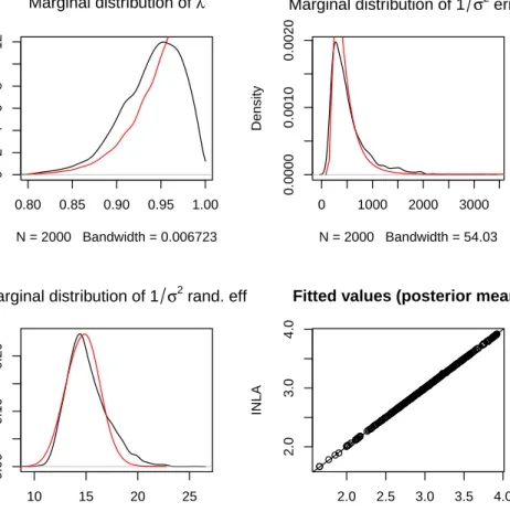
0.80 0.85 0.90 0.95 1.00 0 2 4 6 8 12 Marginal distribution of λ N = 2000 Bandwidth = 0.006723 Density 0 1000 2000 3000 0.0000 0.0010 0.0020

Marginal distribution of 1 σ2 error

N = 2000 Bandwidth = 54.03 Density 10 15 20 25 0.00 0.10 0.20

Marginal distribution of 1 σ2 rand. eff.

N = 2000 Bandwidth = 0.363 Density ● ● ● ●● ● ● ● ●● ● ●●● ●● ● ●●● ● ● ● ●● ● ● ● ●● ●● ●●● ●●● ● ● ● ● ● ● ● ●● ● ● ●●● ● ● ● ● ● ● ● ● ● ● ●● ● ● ●● ● ● ● ●●●● ● ●●●● ● ●● ●●● ●●● ● ● ●●● ● ● ● ●● ● ●● ●●●●●●●●●● ● ●● ●●●●● ● ● ● ●● ● ●● ● ● ●●● ● ● ● ● ● ● ● ● ● ●● ●● ● ● ● ● ● ● ● ● ● ● ● ● ● ● ● ● ● ● ●● ● ●● ● ●● ●● ● ● ●● ● ●● ●● ● ●● ● ● ●●● ● ● ● ● ● ● ●●●● ● ●●● ●● ●● ●● ● ● ● ●●● ● ●● ● ● ●● ●● ● ● ● ● ● ● ●● ● ●● ● ● ●● ●● ● ●● ● ● ●●●● ● ● ● ● ● ● ● ●● ●● ●● ● ● ● ● ●● ● ● ● ● ● ●● ● ● ● ● ●● ● ● ● ● ●● ● ● ● ● ● ● ● ● ● ● ● ● ● ●● ● ● ● ● ● ● ● ●● ● ●● ● ● ●●● ● ● ● ● ● ● ● ● ● ●● ● ●● ● ●●●● ● ● ● ● ● ● ●●● ●● ● ● ●● ● ●●●● ●● ● ●● ●● ● ●●● ● ●●● ● ● ● ● ●●● ● ● ● ● ● ●● ● ● ● ● ●● ● ● ● ● ● ● ● ● ● ● ● ● ● ● ● ● ● ● ●●● ● ●● ● ● ● ● ● ● ●●● ● ● ● ● ● ●● ● ● ● ● ● ● ●● ●● ● ●●●● ●● ● ● ● ●● ● ● ●●●● ● ● ● ●●●●● ● ● ● ● ● ● ● ●●● ● ● ●● ●● ● ●● ● ●● ● ● ● ● ● ● ● ● ● ● ● ● 2.0 2.5 3.0 3.5 4.0 2.0 3.0 4.0

Fitted values (posterior mean)

MCMC

INLA

Figure 7: Comparisson between the posterior marginals of several parameters in Leroux et al.’s model and fitted values with INLA (red) and MCMC (black).

R> library("CARBayes")

R> lcarbayes <- S.CARleroux(form2, data = boston, W = boston.matB,

+ family = "gaussian", burnin = 1000, n.sample = 11000, thin = 5)

Table2 shows point estimates and standard deviations of the fixed effects and parameter λ

(bottom line) in the model. It is clear that there are no significant differences between the estimates computed with MCMC and our method. Furthermore, Figure7shows the marginal distribution of λ and it shows how our estimate is very close to that provided by MCMC. Figure 7 also shows a good agreement between the posterior means of the fitted values. While writting this paper, Lee and Mitchell (2013) have come up with an alternative way of fitting this model using R-INLA and a generic1 latent model. In general, the results obtained for λ with our approach are very similar to the ones obtained with theirs for the Boston housing data.

5.2. Spatial econometrics models

LeSage and Pace (2009) describe in detail a range of models used in spatial econometrics. These models have been developed to make the dependence among the observed values yi

explicit. First of all, spatial dependence can be assumed on the error term (SEM model), so that we have a slightly different model:

y=α+βX+u;u=ρW u+ε (25)

Here the error term uis assumed to have spatial dependence. ρ is a parameter that controls spatial autocorrelation, α is the intercept, X a design matrix of covariates andβ a vector of associated coefficients. ε is an error term which is Gaussian with zero mean and variance-covariance matrix Σ. Here, Σ = σ2In with In being a n×n identity matrix and σ2 is the variance of the error term.

The adjacency matrix W is often taken to be row-standardized (see, for example, Haining 2003) to ensure that ρ is in the interval (−1,1). Also, when ρ is equal to zero there is no spatial dependence.

This can be reformulated as

y =α+βX+ε0 (26)

ε0 is now an error term with a Gaussian distribution with zero mean and variance-covariance matrix Σ =σ2((In−ρW)(In−ρW>))−1. Note that this variance-covariance encodes spatial dependence in a particular way and that this is often referred to as Simultaneous Autoregres-sive (SAR) specification (see, for example,Cressie 1993).

Alternatively, autocorrelation can be modelled explicitly so that the variable response y de-pends on itself. This is the Spatial Lag Model (SLM model) and it can be defined as follows:

y=α+βX+ρW y+ε (27)

This model can be reformulated as

y= (In−ρW)−1(α+βX) +ε0 (28)

where ε0 is a Gaussian term with zero mean and variance-covariance matrix with a SAR specification.

In addition to the previous models, sometimes lagged covariates are added to include the effects of neighboring covariates. This is known as Spatial Durbin Model (SDM) and it is often expressed as

y=ρW y+α+βX+γW X+ε (29)

which leads to

y= (In−ρW)−1(α+βX+γW X) +ε0 (30)

Note that this is like our previous model in Equation28using an extended design matrix that includes bothX and W X.

These models cannot be fitted withR-INLAfor two reasons. First of all, the SAR specification is not implemented, so we cannot consider it for our error terms. Furthermore, it is not possible to define a model where the linear predictor is multiplied by (In−ρW)−1.

Following Section4, it should be noted that, for a fixedρ, these models become standard linear models with a particular (but known) design matrix for the fixed effects and a multivariate Gaussian distribution for the error term with zero mean and variance-covariance matrix. This model can be easily fitted usingR-INLAfor different values ofρ. Note that, according to Haining(2003), ρ is constrained to be in the interval (1/λmin,1/λmax), with λmin and λmax

the minimum and maximum eigenvalues of the adjacency matrix W. For row standardized adjacency matrices we have thatλmax = 1 and thenρ is lower than 1. Furthermore, we are often interested in positive spatial autocorrelation and, in practice, we will assume that ρ is in the interval [0,1).

Finally, we have considered here the Gaussian case, but it is very easy to extend this model to consider other likelihoods. In particular,LeSage, Pace, Lam, Campanella, and Liu (2011) describe a Spatial Probit model where the outcome is whether an event occurred. Hence, the response and the linear predictors are linked via a probit function as follows:

yi =

1 ify_i∗≥0

0 ify_i∗<0 (31)

The previous approach can be used here as well. The same code will still work as we can define a different family and link function to be used when callinginla().

Boston housing data

Here we revisit the Boston housing data to fit the three models on Spatial Econometrics previously described. First of all, it is worth mentioning that each models needs a wrapper function to be fitted for a given value of the spatial autocorrelation parameter ρ. These wrapper functions are included inRpackage R-INLA.

All functions are based on thegeneric0model available inR-INLA. This model implements a multivariate Gaussian random effect with zero mean and precision matrixτ Q. Once ρ is fixed, Q is known and the model can be easily fitted with R-INLA for that value of ρ. We repeat this procedure for different values ofρto obtain a list of fitted models to be combined later.

A simple wrapper function can be defined as follows for the SEM model:

R> semwr.inla <- function(formula, d, W, rho, ...) {

+ IrhoW <- diag(nrow(W)) - rho * W

+ IrhoW2 <- t(IrhoW) %*% IrhoW

+ environment(formula) <- environment()

+ formula <- update(formula, . ~ . + f(idx, model = "generic0",

+ Cmatrix = IrhoW2))

+ res <- inla(formula, data = d, ...)

+ res$logdet <- as.numeric(determinant(IrhoW2)$modulus)

+ res$mlik <- res$mlik + res$logdet/2

+ return(res)

+ }

In the previous code, the precision matrix IrhoW2 is created using the adjacency matrix and the value of ρ and the generic0 model is added to the formula after the fixed effects. As discussed with the Leroux model, the marginal log-likelihood π(y|ρ) (note that now we are conditioning on ρ) is corrected by adding half the log-determinat of (In−ρW>)(In−ρW). Argument ... is used, again, to pass any other options to inla().

Similar wrapper functions can be written for the other models. The functions included in package INLABMA are similar, but include further options, to improve fitting or compute the impacts (see Bivand et al. 2014b, for details).

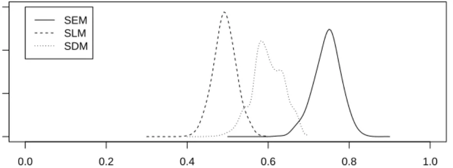
0.0 0.2 0.4 0.6 0.8 1.0 0 5 10 15 ρ π ( ρ |y) SEM SLM SDM

Figure 8: Posterior marginal of the spatial autocorrelation parameter ρ for different spatial econometrics models, Boston housing data.

This is used in the following example to compute the fitted models for the SEM model. Note that herezero.variance is used to set to zero the additional error term which is added by default by R-INLA. Also, the adjacency matrix is taken from the data provided in theboston data set.

R> zero.variance <- list(prec = list(initial = 25, fixed = TRUE)) R> boston.mat <- nb2mat(bostonadj)

R> bmsp <- as(boston.mat, "CsparseMatrix") R> boston$idx <- 1:nrow(boston)

R> fform <- log(CMEDV) ~ CRIM + ZN + INDUS + CHAS + I(NOX^2) + I(RM^2) +

+ AGE + log(DIS) + log(RAD) + TAX + PTRATIO + B + log(LSTAT)

Next, we define a fine grid to give values toρ and compute the different models under these values. Again, we have usedmclapplyto speed up computations.

R> rrho1 <- seq(0.5, 0.9, len = 20)

R> semmodels <- mclapply(rrho1, function(rho) {

+ sem.inla(fform, d = as.data.frame(boston), W = bmsp, rho = rho,

+ family = "gaussian", impacts = FALSE,

+ control.family = list(hyper = zero.variance),

+ control.predictor = list(compute = TRUE),

+ control.compute = list(dic = TRUE, cpo = TRUE),

+ control.inla = list(print.joint.hyper = TRUE))

+ })

Following this, we need to combine the different models to obtain the final model by Bayesian model averaging. As in the example using the Leroux model, we will take a uniform prior on

ρ and set the third argument in the following function to log(1) = 0.

R> bmasem <- INLABMA(semmodels, rrho1, 0, impacts = FALSE)

bmasem is similar to the object returned by inla() and it includes the posterior marginals and summary statistics for ρ.

SLM and SDM models can be fitted using similar code. In the case of the SLM, first we compute the design matrix (of the fixed effects) to be used later when fitting the models. This will speed up the computations.

R> mmatrix <- model.matrix(fform, as.data.frame(boston)) R> rrho2 <- seq(0.3, 0.6, len = 20)

R> slmmodels <- mclapply(rrho2, function(rho) {

+ slm.inla(form, d = as.data.frame(boston), W = bmsp, rho = rho,

+ mmatrix = mmatrix, family = "gaussian", impacts = TRUE,

+ control.family = list(hyper = zero.variance),

+ control.predictor = list(compute = TRUE),

+ control.compute = list(dic = TRUE, cpo = TRUE),

+ control.inla = list(print.joint.hyper = TRUE))

+ })

R> bmaslm <- INLABMA(slmmodels, rrho2, 0, impacts = FALSE)

In the case of the SDM, it is very helpful to compute X and W X beforehand to reduce computation time, as this is common to all the fitted models regardless of the value ofρ. This can be later passed to wrapper function sdm.inla.

R> mmW <- bmsp %*% mmatrix[, -1]

R> mmatrixsdm <- cbind(mmatrix, as.matrix(mmW)) R> rrho3 <- seq(0.4, 0.7, len = 20)

R> sdmmodels <- mclapply(rrho3, function(rho) {

+ sdm.inla(form, d = as.data.frame(boston), W = bmsp, rho = rho,

+ mmatrix = mmatrixsdm, family = "gaussian", impacts = TRUE,

+ control.family = list(hyper = zero.variance),

+ control.predictor = list(compute = TRUE),

+ control.compute = list(dic = TRUE, cpo = TRUE),

+ control.inla = list(print.joint.hyper = TRUE))

+ })

R> bmasdm <- INLABMA(sdmmodels, rrho3, 0, impacts = FALSE)

As we have seen in the previous examples, combining the different values for the different values of ρ provides accurate estimates of the posterior marginals for the model parameters. The estimates of the marginals of ρ can be found in Figure 8.

6. Discussion

The integrated nested Laplace approximation has provided a new paradigm to model fitting in Bayesian analysis. By focusing on the marginals and providing an interesting computational approach, it has become a reasonable and faster alternative to MCMC. Furthermore, the

R-INLApackage makes model fitting in Ra very simple task. AlthoughR-INLA implements some key models, there are some others that have not been implemented yet. In addition, it is not easy to implement completely new models within R-INLA. Latent mixture models are an important example of models that cannot be fitted with R-INLA.

In this paper we have shown an innovative approach to model fitting with INLA andR-INLA which increases the number of latent models that can be fitted with INLA. We have been able to do so by fitting conditional models on some model parameters and combining the resulting models using simple methods for Bayesian model averaging. We have considered the case in which conditioning is carried out on a single parameter but our approach can be easily extended to the case of more than one parameter.

Given that the different models can be run in parallel, this is not a real computational burden. In our examples, 20 models seemed to be enough to obtain good approximations. Implement-ing new models is very simple and the wrapper functions included in the examples and the INLABMApackage provide templates to start with.

Other computationally efficient approaches for Bayesian inference on spatial models include, for example,RStan(StanDevelopment Team 2013). It provides an efficient MCMC algorithm and provides a good number of options for Gaussian processes which can be used to implement some of the models described in this paper. It is worth mentioning that RStan models are not based onRcode but onC++code that is compiled once the main model is defined. We have shown that this is a practical approach using different examples in spatial statistics. Similarly, complex spatio-temporal models could be fitted using a similar approach. However, it should be noted that our approach can be extended to other areas.

Acknowledgments

We would like to thank Duncan Lee and Lola Ugarte for their help and comments on how to fit the Leroux model with R-INLA. Virgilio G´omez-Rubio acknowledges partial funding from project PPIC-2014-001, funded by Consejer´ıa de Educaci´on, Cultura y Deportes (JCCM, Spain) and FEDER.

References

Baddeley A, Turner R (2005). “spatstat: AnRPackage for Analyzing Spatial Point Patterns.”

Journal of Statistical Software,12(6), 1–42. URL http://www.jstatsoft.org/v12/i06/. Besag J, York J, Molli´e A (1991). “Bayesian Image Restoration, with Two Applications in

Spatial Statistics.”Annals of the Institute of Statistical Mathematics,43(1), 1–59.

Bivand R (2014). spdep: Spatial Dependence: Weighting Schemes, Statistics and Models. R

package version 0.5-74, URLhttp://CRAN.R-project.org/package=spdep.

Bivand R, Keitt T, Rowlingson B (2014a). rgdal: Bindings for the Geospatial Data Ab-straction Library. Rpackage version 0.8-16, URLhttp://CRAN.R-project.org/package= rgdal.

Bivand R, Lewin-Koh N (2014). maptools: Tools for Reading and Handling Spatial Objects.

Rpackage version 0.8-30, URLhttp://CRAN.R-project.org/package=maptools.

Bivand RS, G´omez-Rubio V, Rue H (2014b). “Approximate Bayesian Inference for Spatial Econometrics Models.”Spatial Statistics,9, 146–165.

Bivand RS, Pebesma E, G´omez-Rubio V (2013). Applied Spatial Data Analysis with R. 2nd edition. Springer-Verlag, New York.

Blangiardo M, Cameletti M, Baio G, Rue H (2013). “Spatial and Spatio-Temporal Models withR-INLA.”Spatial and Spatio-Temporal Epidemiology,4, 33 – 49.

Cameletti M, Lindgren F, Simpson D, Rue H (2013). “Spatio-Temporal Modeling of Particu-late Matter Concentration through the SPDE Approach.”Advances in Statistical Analysis,

97(2), 109–131.

Christensen OF, Ribeiro PJ (2002). “geoRglm – A Package for Generalised Linear Spatial Models.”RNews,2(2), 26–28. URLhttp://CRAN.R-project.org/doc/Rnews/.

Cressie NAC (1993). Statistics for Spatial Data. John Wiley & Sons, New York. Diggle PJ, Ribeiro PJ (2007). Model-Based Geostatistics. Springer-Verlag, New York. Eidsvik J, Finley AO, Banerjee S, Rue H (2012). “Approximate Bayesian Inference for Large

Spatial Datasets Using Predictive Process Models.”Computational Statistics & Data Anal-ysis,56(6), 1362–1380.

G´omez-Rubio V, Bivand R (2014). INLABMA: Bayesian Model Averaging with INLA. R

package version 0.1-5, URL http://CRAN.R-project.org/package=INLABMA.

G´omez-Rubio V, Bivand RS, Rue H (2014a). “Estimating Spatial Econometrics Models with Integrated Nested Laplace Approximation.”Submitted for publication.

G´omez-Rubio V, Bivand RS, Rue H (2014b). “Spatial Models Using Laplace Approximation Methods.” In MM Fischer, P Nijkamp (eds.),Handbook of Regional Science, pp. 1401–1417. Springer-Verlag, New York.

Haining R (2003). Spatial Data Analysis: Theory and Practice. Cambridge University Press, Cambridge.

Harrison D, Rubinfeld DL (1978). “Hedonic Housing Prices and the Demand for Clean Air.”

Journal of Environmental Economics and Management,5(1), 81–102.

Held L, Sch¨odle B, Rue H (2010). “Posterior and Cross-Validatory Predictive Checks: A Comparison of MCMC and INLA.” In T Kneib, G Tutz (eds.), Statistical Modelling and Regression Structures – Festschrift in Honour of Ludwig Fahrmeir, pp. 91–110. Springer-Verlag, Berlin.

Hoeting J, Madigan D, Raftery A, Volinsky C (1999). “Bayesian Model Averaging: A Tuto-rial.”Statistical Science,14(4), 382–401.

Hossain MM, Lawson AB (2009). “Approximate Methods in Bayesian Point Process Spatial Models.”Computational Statistics & Data Analysis,53(8), 2831–2842.

Kahle D, Wickham H (2013). “ggmap: Spatial Visualization withggplot2.” The R Journal,

5(1), 144–162. URLhttp://journal.R-project.org/archive/2013-1/kahle-wickham. pdf.

Lee D (2013). “CARBayes: An R Package for Bayesian Spatial Modeling with Conditional Autoregressive Priors.” Journal of Statistical Software, 55(13), 1–24. URL http://www. jstatsoft.org/v55/i13/.

Lee D, Mitchell R (2013). “Locally Adaptive Spatial Smoothing Using Conditional Auto-Regressive Models.”Journal of the Royal Statistical Society C,62(4), 593–608.

Leroux B, Lei X, Breslow N (1999). “Estimation of Disease Rates in Small Areas: A New Mixed Model for Spatial Dependence.” In M Halloran, D Berry (eds.), Statistical Models in Epidemiology, the Environment and Clinical Trials, pp. 135–178. Springer-Verlag, New York.

LeSage J, Pace RK (2009). Introduction to Spatial Econometrics. Chapman & Hall/CRC, Boca Raton.

LeSage JP, Pace RK, Lam N, Campanella R, Liu X (2011). “New Orleans Business Recovery in the Aftermath of Hurricane Katrina.”Journal of the Royal Statistical Society A,174(4), 1007–1027.

Lindgren F, Rue H (2015). “Bayesian Spatial Modelling with R-INLA.”Journal of Statistical Software,63(19), 1–25. URL http://www.jstatsoft.org/v63/i19/.

Lindgren F, Rue H, Lindstr¨om J (2011). “An Explicit Link between Gaussian Fields and Gaussian Markov Random Fields: The SPDE Approach.” Journal of the Royal Statistical Society B,73(4), 423–498.

Martino S, Rue H (2010). “Case Studies in Bayesian Computation Using INLA.” In P Man-tovan, P Secchi (eds.), Complex Data Modeling and Computationally Intensive Statistical Methods, Contributions to Statistics, pp. 99–114. Springer-Verlag, New York.

Neuwirth E (2014). RColorBrewer: ColorBrewerPalettes. Rpackage version 1.1-2, URL http://CRAN.R-project.org/package=RColorBrewer.

Pace RK, Gilley OW (1997). “Using the Spatial Configuration of the Data to Improve Esti-mation.”Journal of the Real Estate Finance and Economics,14(3), 333–340.

RCore Team (2014). R: A Language and Environment for Statistical Computing. R Founda-tion for Statistical Computing, Vienna, Austria. URLhttp://www.R-project.org/. Ribeiro PJ, Diggle PJ (2001). “geoR: A Package for Geostatistical Analysis.” R News,1(2),

15–18. URL http://CRAN.R-project.org/doc/Rnews/.

Rue H, Held L (2005).Gaussian Markov Random Fields – Theory and Applications. Chapman & Hall, New York.

Rue H, Martino S, Chopin N (2009). “Approximate Bayesian Inference for Latent Gaus-sian Models by Using Integrated Nested Laplace Approximations.” Journal of the Royal Statistical Society B,71(2), 319–392.

Rue H, Martino S, Lindgren F, Simpson D, Riebler A, Krainski ET (2014). INLA: Functions Which Allow to Perform a Full Bayesian Analysis of Structured Additive Models Using Integrated Nested Laplace Approximaxion. R package version 0.0-1406288160, URLhttp: //www.r-inla.org/.

Ruiz-Cardenas R, Krainski ET, Rue H (2012). “Direct Fitting of Dynamic Models Using Integrated Nested Laplace Approximations – INLA.” Computational Statistics & Data Analysis,56(6), 1808–1828.

Schr¨odle B, Held L (2010). “A Primer on Disease Mapping and Ecological Regression Using INLA.”Computational Statistics,26(2), 241–258.

Schr¨odle B, Held L (2011). “Spatio-Temporal Disease Mapping Using INLA.”Environmetrics,

22(6), 725–734.

Schr¨odle B, Held L, Riebler A, Danuser J (2011). “Using Integrated Nested Laplace Approx-imations for the Evaluation of Veterinary Surveillance Data from Switzerland: A Case-Study.”Journal of the Royal Statistical Society C,60(2), 261–279.

Spiegelhalter DJ, Best NG, Carlin BP, Van der Linde A (2002). “Bayesian Measures of Model Complexity and Fit.”Journal of the Royal Statistical Society B,64(4), 583–616.

StanDevelopment Team (2013). “Stan: AC++Library for Probability and Sampling, Version 1.3.” URL http://mc-stan.org/.

Umlauf N, Adler D, Kneib T, Lang S, Zeileis A (2015). “Structured Additive Regression Models: An R Interface to BayesX.” Journal of Statistical Software, 63(21), 1–46. URL http://www.jstatsoft.org/v63/i21/.

Umlauf N, Kneib T, Lang S, Zeileis A (2013). R2BayesX: Estimate Structured Additive Regression Models with BayesX. Rpackage version 0.3-1, URL http://CRAN.R-project. org/package=R2BayesX.

Wickham H (2009). ggplot2: Elegant Graphics for Data Analysis. Springer-Verlag, New York. URL http://had.co.nz/ggplot2/book/.

Wood SN (2006). Generalized Additive Models: An Introduction with R. Chapman & Hall/CRC, Boca Raton.

Affiliation: Roger S. Bivand

Department of Economics

NHH Norwegian School of Economics Helleveien 30

N-5045 Bergen, Norway

E-mail: [email protected] Virgilio G´omez-Rubio

Department of Mathematics School of Industrial Engineering University of Castilla-La Mancha 02071 Albacete, Spain