Exascale Storage Systems -- An Analytical Study of Expenses

Exascale Storage Systems – An Analytical Study of Expenses

The computational power and storage capability of supercomputers are growing at a differ-ent pace, with storage lagging behind; the widening gap necessitates new approaches to keep the investment and running costs for storage systems at bay. In this paper, we aim to unify previous models and compare different approaches for solving these problems. By extrapolating the char-acteristics of the German Climate Computing Center’s previous supercomputers to the future, cost factors are identified and quantified in order to foster adequate research and development. Using models to estimate the execution costs of two prototypical use cases, we are discussing the potential of three concepts: re-computation, data deduplication and data compression.

Keywords: Parallel I/O, Exascale, data center, storage expenses.

1. Introduction

Supercomputers combine the power of thousands of computers to provide enough computational power to tackle complex scientific problems. They are used to conduct large-scale computations and simulations of complex systems from basically all branches of the natural and technical sciences, such as meteorology, climatology, particle and astro physics. As these simulations have become more accurate and thus realistic over the last years, their demands for computational power have also increased. This, in turn, has also caused the simulation results to grow in size, increasing the demands for huge storage systems. High performance I/O is an important aspect, because storing and retrieving such large amounts of data can greatly affect the overall performance of these applications.

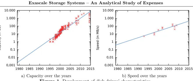
Processor speed [26] and disk capacity [11, 30] have roughly increased by factors of 500 and 100 every 10 years, respectively. The speed of disks, however, grows more slowly; this can be seen in Figures 1a and 1b, which show the increase in disk capacity and speed from roughly the same period of time. Early disks in 1989 delivered about 0.5 MB/s, while current disks manage around 200 MB/s [29]. This corresponds to a 400-fold increase of throughput over the last 25 years. Even newer technologies such as solid-state drives (SSDs) only offer throughputs of around 600 MB/s, resulting in a total speedup of 1,200. In comparison, over the same period of time, the computational power increased by a factor of 1,000,000 for supercomputers due to increasing investments. We are approaching ExaFLOPS performance by the end of the decade. While this problem cannot be solved without major breakthroughs in hardware technology, it is necessary to use the storage hardware as efficiently as possible to alleviate its effects. Moreover, the growth of disk capacity has recently also started to slow down. While the same is true for processor clock rate, this particular problem is being compensated for by growing numbers of increasingly cheap processor cores. Additional investment is required to keep up with the advancing processing power. The outcome of this is that it is not possible to increase storage speed and capacity by the same factor as processing power when keeping investment constant.

Due to the increasing electricity footprints, energy used for storage represents an important portion of the Total Cost of Ownership (TCO) [7]. For instance, the German Climate Computing Center’s (DKRZ) storage system is using 7,200 disks to provide a 5.6 PB file system for earth system science. Assuming a power consumption of 20 W for a disk, this results in energy costs of 144,000eper year for the disks alone.

0,001 0,01 0,1 1 10 100 1.000 10.000

1980 1985 1990 1995 2000 2005 2010 2015

Capacit

y (in GB

)

a) Capacity over the years

0,001 0,01 0,1 1 10 100 1.000 10.000

1980 1985 1990 1995 2000 2005 2010 2015

Speed

(in MB/s)

b) Speed over the years

Figure 1.Development of disk drives’ characteristics

It is obvious that the increasing demand for storage, combined with the growing gap between processor and storage development, makes it necessary to take action to be able to build balanced supercomputers in the future. The contributions of this paper in this regard are: 1) The prediction of future supercomputers’ characteristics for DKRZ. 2) A simplified cost model for running an application, focused on costs for storage and long-term data archival. 3) The quantification of several strategies to reduce data volume. Here, we continue our research on Total Cost of Ownership (TCO) of HPC centers [27, 28].

The rest of this paper is structured as follows: First, the characteristics of future systems at DKRZ are discussed and predicted in Section 2. Then in Section 3, scientific I/O is characterized and two typical simulation experiments are introduced. Additionally, a few observations from the system perspective are provided. The basic model for estimating costs of a job is introduced in Section 4. This model is then applied to typical runs estimating their costs. At last, a more sophisticated cost analysis for long-term data storage is conducted. In Section 5, the concepts of re-computation, deduplication, compression and user-education are introduced and their benefit for future systems is quantified and discussed. Finally, in Section 6 we summarize our findings and identify future work.

2. Characteristics of Future Systems

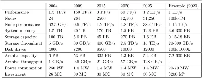
Table 1 shows the characteristics of the previous (2004) and current (2009) DKRZ systems as well as strawmans for future systems (2015, 2020 and 2025)3_{. An estimate for the investment costs and} power consumption for DKRZ is listed in Table 2. One assumption of the extrapolation is that costs stay on the current level. The column “Exascale System” lists the range of characteristics of an Exascale class system as projected by experts [3, 5, 8–10, 17]; note that these predictions vary strongly over time. We approximate the performance characteristics for the next generations according to an extrapolation of trends and hardware roadmaps4_{. A brief explanation of the} improvement factors assumed and rationales for them are given in the following:

• For the processor performance, a 20x improvement with every new generation is anticipated, leading to Exascale performance in 2025. This matches the trend that the DKRZ system is about 5 years behind the fastest supercomputer.

3_{The typical procurement cycle is 5 years.}

• The increase in compute performance can be facilitated by increasing the sheer performance per core, node or the number of nodes. Between between 2004 and 2015, the number of nodes increased by 10x while the number of processor cores per node only increased slightly. We assume, in 2020 and 2025 the intra-node concurrency in densely packed nodes will advance significantly, therefore, the required number of nodes will advance moderately (by 5x and 2.5x, respectively). A transition to accelerators will increase intra-node concur rency significantly, for example. The achieved performance per node of the 2020 system is similar to the performance of the aggressively designed strawman architecture in [17] (4.5 TF/s); with multiple GPUs per node, a performance level which is achievable today.

• Storage throughput experienced a big jump of 13x in the 2015 system which is too optimistic for the future. We expect it to flatten out to 6x for the next few generations of systems: Historically, the performance of disks grew by about 27 % per year or 3.34x in 5 years (see Figure 1b). Current bottlenecks degrade raw performance to a mere 48 MB/s per disk; improvements in hardware and software need to exploit available performance better. We expect a 50 % gain of overall storage performance by improving scheduling with techniques such as burst-buffers, an additional 20 % will be gained by the extra disks.

• Storage capacity may improve by 6x with every new generation. This is mainly motivated by the advances in disk technology. Based on the trend, capacity will increase by 54.4 % annually (see Figure 1a); according to Gartner [22] the annual growth rate of high-density enterprise disks will even be 66.7 % until 2018. If the trend in areal density continues, disks with more than 700 TB would arise in 2025. To prove the storage capacity, the 2025 system requires 133 TB disks, which – by this extrapolation – will be available. Nevertheless, the number of deployed disks will increase by 20 % every generation; to keep the current power budget (as assumed), optimizations in energy efficiency must reduce power consumption. One recent technological advancement which bridges the gap to the next generation system are helium-filled hard disks. However, due to the slower increase in performance, the rebuild time of such a disk would be extensive (almost 3 days).

• Currently, 7 StorageTek silos provide 67,000 slots and 80 tape drives – even if no new libraries are bought, the archive capacity can be increased significantly. The technology offers a raw capacity of 800 GB, 1,500 GB and 2,500 GB for LTO-Ultrium 4, 5 and 6, respectively. Based on the LTO roadmap, the characteristics of a future archive can be approximated well; a doubling of capacity every 2.5 years is expected. Note that this assumption lags behind the historical doubling of disk storage capacity every 15 months, but matches the past development of the LTO standard. Between LTO-4 and LTO-8, throughput is predicted to increase from 120 MB/s to 472 MB/s. With LTO-6, the ALDC compression scheme is switched to LTO-DC which is predicted to increase the average compression ratio from 2 to 2.5.

• The available budget increased only slightly5_{, therefore, a similar level of investment and} power consumption must be kept. One interesting observation validating the potential char-acteristics of the 2020 system: if an Exascale system will be deployed in 2020 with a power consumption of 20 MW, the 2020 system with 60 PF/s will have an power consumption of 1.2 MW; which is a bit lower than the value indicated in the table.

2004 2009 2015 2020 2025 Exascale (2020) Performance 1.5 TF/s 150 TF/s 3 PF/s 60 PF/s 1.2 EF/s 1 EF/s

Nodes 24 264 2500 12,500 31,250 100k-1M

Node performance 62.5 GF/s 0.6 TF/s 1.2 TF/s 4.8 TF/s 38.4 TF/s 1-15 TF/s System memory 1.5 TB 20 TB 170 TB 1.5 PB 12.8 PB 3.6-300 PB Storage capacity 100 TB 5.6 PB 45 PB 270 PB 1.6 EB 0.15-18 EB Storage throughput 5 GB/s 30 GB/s 400 GB/s 2.5 TB/s 15 TB/s 20-300 TB/s Disk drives 4000 7200 8500 10000 12000 100k-1000k Archive capacity 6 PB 53 PB 335 PB 1.3 EB 5.4 EB 7.2-600 EB Archive throughput 1 GB/s 9.6 GB/s 21 GB/s 57 GB/s 128 GB/s

-Power consumption 250 kW 1.6 MW 1.4 MW 1.4 MW 1.4 MW 20-70 MW Investment 26 Me 30 Me 30 Me 30 Me 30 Me $200 M4

Table 1. DKRZ System characteristics; future systems are a potential scenario

Investment Power consumption

Compute 15.75 Me 1100 kW

Network 5.25 Me 50 kW

Storage 7.5 Me 250 kW

Archive 5 Me 25 kW

Burst-Buffer 2 Me 25 kW

Table 2. Potential investment costs and power consumptions for DKRZ for all future systems

the DKRZ could archive the capacity of the file system per year and keep it for 10 years, which will not be feasible in 2025 any more. Also, the extrapolated throughput of the archive will not suffice to store the data. While it took about 3.6 years – which is enough time for the next procurement – in 2009 to fill the whole archive, the 2015 system will require 12 years already. With the 2025 system and its 128 GB/s of archive throughput, it would take 32 years to fill it completely. However, by increasing the number of tape drives from 80 to the maximum of 448 (5.5x), a large fraction of the required performance can be covered. 2) The speed of computation increases much faster (by 20x) than the storage capacity (5x). Thus, to maintain balance, in the next generations the generated data volume per FLOP must be reduced to one quarter.

With such a system, the often discussed issue of checkpointing is not relevant for DKRZ: Over the time, full system checkpointing increases slightly from 667 s in 2009 to 853 s in 2025. Since most users perform application-specific checkpointing and mostly run small scale configurations, only a fraction of this time is required. 6

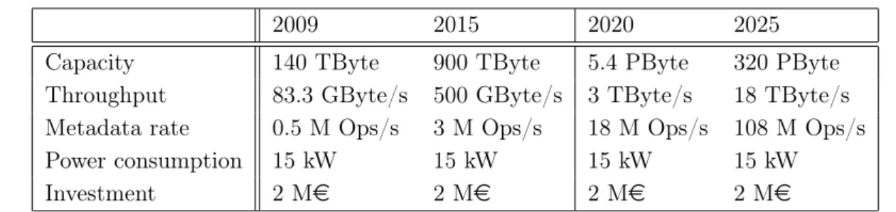
2.1. Burst-Buffer

There have been many thoughts in the HPC community about the potential use of storage class memory in Exascale systems. One scenario is to deploy it as globally accessible cache like in the FastForward I/O effort of Intel, the HDF group and others [5]. Another potential scenario is to utilize node-local or rack-local storage as a new storage tier.

2009 2015 2020 2025 Capacity 140 TByte 900 TByte 5.4 PByte 320 PByte Throughput 83.3 GByte/s 500 GByte/s 3 TByte/s 18 TByte/s Metadata rate 0.5 M Ops/s 3 M Ops/s 18 M Ops/s 108 M Ops/s

Power consumption 15 kW 15 kW 15 kW 15 kW

Investment 2 Me 2 Me 2 Me 2 Me

Table 3. Potential burst-buffer characteristics; future systems are extrapolated from the current trend

Deploying non-volatile memory at DKRZ could increase the efficiency of the disk-based storage tier which is required to achieve the 6x performance gain as discussed in Section 2. One concept is to modify applications to use a burst-buffer API to explicitly manage a working set of input data prior job execution. Also, temporarily storing data on the faster storage until it is post-processed is an option. Finally, a transparent fast tier for small files and metadata would reduce the seeks on the disks, allowing them to increase their sustained throughput. This approach requires a tight integration into the file system or use of a middleware that takes care of blending the namespaces together. Such a policy could be potentially based on the file extension or on hints such as the selected stripe count in Lustre. Based on the current system usage (see Section 3.3), a 400 GB SSD tier could host all of DKRZ’s 50 million files with a size below 8 KiB. Also, with additional 60 TB and 70 TB, files below 1 MiB and 2 MiB could be stored, respectively. Based on our system’s dimension, deploying 1,000 non-volatile memory devices in 25–50 servers seems possible. Inspired by the characteristics of the Intel DC S3700 enterprise SSD7_, potential burst-buffer characteristics are extrapolated and listed in Table 3. With 2 % of the disks’ capacity, the burst-buffer would be rather small, yet all small files could be located there easily – even if their number keeps growing according to the current trend. Sustained performance of this system might only be slightly higher than the sustained performance of the disk tier. However, as discussed it could be used to guarantee a better sustained performance of the disks.

3. Scientific I/O

The output of typical scientific applications can be classified by the semantics of the data. There are four kinds: A data product is data which is further processed for scientific discovery;

diagnostic datacontains information about the execution of the application – it helps to check correctness of a run; the traditionalcheckpoint; andout-of-core data. In this paper, we focus on earth system models; out-of-core computation and other cases are not discussed further, as these are non-typical scenarios for these models.

Weather and climate models periodically store scientific variables – such as temperature and humidity – for each of the simulated domains (cells of a grid). Based on the resolution of the domain decomposition and period of the I/O stepping, the produced data volume can vary drastically. Usually, the data products are kept and archived; sometimes selected checkpoints are also archived because re-starting a 1,000 year simulation from scratch takes considerable time. Diagnostic data can theoretically be deleted after the validity of the run has been checked.

In the scientists’ workflow, the data products are often provided to the community and analyzed with different post-processing tools. They are often stored in databases such as the World Data Center for Climate (WDCC) for easier accessibility by other scientists. Recently, big data techniques are discussed to identify interesting phenomena in these large data sets.

In the data model, we classify I/O that is needed to drive a model asstatic I/O; it consists of I/O required for initialization (grid, forcing data), potential data for assimilation and the final output. Its opposite isperiodic output, in which a simulation stores variables periodically. Note that the period can depend on the variable. Next, two prototypical experiments are discussed.

3.1. Use-Case: CMIP5

As part of the assessment report of the Intergovernmental Panel on Climate Change (IPCC), the Coupled Model Intercomparison Project Phase 5 (CMIP5) [1] compares the predictions of a variety of climate models for a common set of experiments. More than 10.8 million processor hours of the DKRZ’s supercomputer were used for the German contribution to CMIP5. In to-tal, 482 runs have been conducted simulating a total of 15,280 years. Depending on the model (atmosphere, ocean, land or chemistry), the output period can fluctuate from six model hours to one model month. Together with checkpoints, a data volume of more than 640 TB has been created. During post-processing, the data products are further refined into 55 TB of data which is then published in scientific databases.

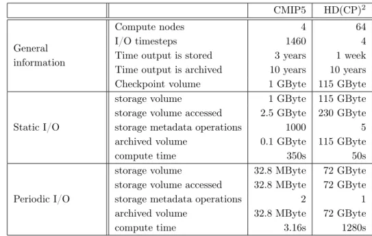
While there are different experiments, we will only discuss a prototypical low-resolution configuration accounting for 12,229 simulated years: A run for a year takes about 1.5 hours on the 2009 system and finishes by creating a checkpoint. The simulation is continued in another job that restarts from the checkpoint; the application-specific checkpointing of the model components occupies 4 GB. Every 10th checkpoint is kept and archived. A month of simulation accounts for 4 GB of data; about half of it is due to storing values in 6 hour periods; for simplicity, we will assume the monthly data volume is included in the 6 hour means. The high number of metadata operations on the file system by the fixed execution is caused by listing the directory with the created artifacts of the job series and more than 100 accessed files. In order to validate data quality and refine post-processing, the data was stored on the file system for almost three years, after which it was archived for 10 years. Relevant statistics are provided in Table 4.

3.2. Use-Case: HD(CP)2

The High Definition Clouds and Precipitation for Climate Prediction (HD(CP)2_{) is a research}

CMIP5 HD(CP)2

General information

Compute nodes 4 64

I/O timesteps 1460 4

Time output is stored 3 years 1 week Time output is archived 10 years 10 years Checkpoint volume 1 GByte 115 GByte

Static I/O

storage volume 1 GByte 115 GByte storage volume accessed 2.5 GByte 230 GByte storage metadata operations 1000 5 archived volume 0.1 GByte 115 GByte

compute time 350s 50s

Periodic I/O

storage volume 32.8 MByte 72 GByte storage volume accessed 32.8 MByte 72 GByte storage metadata operations 2 1 archived volume 32.8 MByte 72 GByte

compute time 3.16s 1280s

Table 4. Job information for a prototypical run of a model configuration on the DKRZ 2009 system

3.3. System’s Perspective

From a data center’s perspective, it is not yet possible to track the scientific workflow directly. An analysis of the system’s status quo can still provide interesting insights regarding the usage of the provided machinery. With the help of monitoring tools, the utilization can be understood better; this information can be used to support decision making for future procurements. For example, on our current system, the sustained throughput of the file system is about 15 GB/s; additionally, the deployed data compression scheme in the tape library achieves a space saving of about 30 % for our workload. Moreover, it may help directing optimization efforts towards the most valuable system aspects and illustrates the demand for user education. A few insights on user behavior are provided in the following:

To understand the demand of scientists better, the file size distribution and file types are analyzed. The following analysis covers the home and project folders with 3.8 PB of data. Overall, 155,000,000 files are stored; their size is distributed as follows: 28 %≤8 KiB, 76 %≤1 MiB, 90 % ≤ 2 MiB, 99.8 % ≤1 GiB and a few thousand files ≥ 8 GiB. Small files can be explained partly by application code and compilation artifacts; version control with Subversion also increases the amount of tiny files significantly.

These few examples highlight the importance of systematic monitoring of inefficient use, which must be done on billions of files in Exascale systems.

4. Modelling Storage Costs

Various cost models of a system have emerged in literature, each developed for a certain purpose. Hardy et al. designed a tool covering many design aspects for a data center [13]. There are also models describing the costs for executing a parallel application but only a few cover storage in more detail. It is also interesting to analyze the costs of storing data forever, which is possible to quantify under the assumption of unlimited increase in areal density; according to Goldstein in 2011, the cost of conserving 1 TB of data was quantified to be about $5000 [12]. Of course, the price decreases over time – thus, the later data is stored, the cheaper it is – but the more we want to store. We have previously modeled energy consumption for storing scientific data [18]. The model introduced in Equations (4.1) and (4.5) is a simplified model – approximating the costs for running an application and storing data. With this model, we also unify the previously developed models for the purpose of analyzing several Exascale I/O scenarios.

costs(job) =costscompute(job) +costsstorage(job) +costsarchive(job) (4.1)

rCosts(component) =investmentcomponent

systemlif eT ime

+P(component)_·energyCosts (4.2)

costscompute(job) =rCosts(compute)·

jobnodes

systemnodes ·

jobcompute_time (4.3)

costsstorage(job) =rCosts(storage)·

_job

volume

storagecapacity·

jobtime_stored+job_storagevolume_accessed throughput

+jobmetadata_accesses

storagemetadata_rate

(4.4)

costsarchive(job) =

_{rCosts(archive)}

archiveslot_countjobarchival_time+costsmedia

_job

archival_volume

mediacapacity (4.5)

costscheckpoint(job) =

checkpointvolume

storagethroughput ·rCosts(storage) +rCosts(compute)·

jobnodes

systemnodes·

checkpointvolume

min jobnodes·storagethroughput_per_node, storagethroughput

(4.6)

In the model, the variable rCosts represents the running cost for completely utilizing one

understand their impact better. In the archive costs, the number of tape media required to store the data is budgeted (see Equation (4.5)). The costs for checkpoints are given in Equation (4.6); we assume the I/O must be done synchronously and the computation of the application will not continue during checkpointing. The second summand covers the additional costs of the idle compute system; the idle time depends on the time needed to persist the checkpoint.

The model implies several basic assumptions and restrictions: Maintenance by the vendor is usually included in the acquisition costs and, therefore, can be taken into account. Acquisi-tion costs of the data center building are not covered but this investment could be distributed among the component costs. Staff expenses for maintaining the data center are not covered but could be treated in a similar fashion as the facility. The costs for network infrastructure and its utilization are not covered. I/O is not interfering with the compute performance and is com-pletely hidden by using asynchronous techniques; costs for synchronous I/O could be computed using Equation (4.6). While the costs for tape drives could be included in the tape archive costs; the migration of data usually conducted between tape generations is not performed. Tape com-pression is not covered explicitly by the model but could be addressed by increasing the tapes’ capacity virtually. The significant effort of application scientists to port and optimize code for a new system is out of scope of this model as it is hard to capture. Still, by carefully modifying the input variables, it can be adjusted to many scenarios easily. Network costs, for example, could be integrated into the computational costs. The model does not cover expenses caused by idling compute nodes or empty storage space. However, the fraction of costs induced by overprovision-ing of hardware could be multiplied to a job’s cost. For example, data centers may observe a utilization of 95% of the compute nodes and 85% of storage space.

4.1. Predicted Execution Costs

Based on the cost model, the current and future costs of the CMIP5 and HD(CP)2 _{runs can}

be approximated. The required job information of the models are provided in Table 4; results of the forecast are shown in Table 5. Note that the model assumes the number of nodes scales with the required peak-performance of the future nodes; thus, the number of them required to run HD(CP)2 _{degrades from 64 to 32 nodes in 2015, eight nodes in 2020 and one node in}

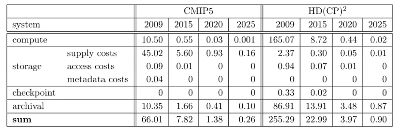
2025. Storage costs from Equation (4.4) are split into three parts: The supply costs (while data occupies capacity but is not used), costs for accessing data and meta data. It can be observed that the storage supply costs are a large fraction of the overall costs for the CMIP5 experiments – keeping the data accessible on disk is the cost driver. The archival costs are in the order of the computation costs. For HD(CP)2, the archival costs are currently about half the execution costs. With future systems, the fraction of storage and archival costs increases and dominates the overall costs by far. In both experiments, the costs for synchronous checkpointing is negligible; forHD(CP)2, it accounts for less than 0.2 % of the computation costs. These predictions clearly indicate the need to reduce the costs for supplying storage space but still retaining science quality.

4.2. Long-term Data Archival

CMIP5 HD(CP)2

system 2009 2015 2020 2025 2009 2015 2020 2025 compute 10.50 0.55 0.03 0.001 165.07 8.72 0.44 0.02

storage

supply costs 45.02 5.60 0.93 0.16 2.37 0.30 0.05 0.01 access costs 0.09 0.01 0 0 0.94 0.07 0.01 0

metadata costs 0.04 0 0 0 0 0 0 0

checkpoint 0 0 0 0 0.33 0.02 0 0

archival 10.35 1.66 0.41 0.10 86.91 13.91 3.48 0.87

sum 66.01 7.82 1.38 0.26 255.29 22.99 3.97 0.90

Table 5. Costs for one simulation run (in e)

costs=

∞ X

y=0

annualCosts_·size capacity0·1.54y

= annualCosts·size

capacity0 · ∞ X

y=0

1 1.54

y

= annualCosts·size

capacity0 ·

1 1_−1.1₅₄ =

annualCosts·size capacity0 ·

2.84

(4.7)

year, the aggregated costs for storing data forever can be computed according to Equation (4.7). In the following, we will approximate the costs for a particular setting: we assume 400efor a 6 TB enterprise disk with a transfer rate of 216 MiB/s. Additionally, for the server infrastructure and regular server and infrastructure updates every five years, 100e are added to the disk’s expenses. Personnel and facility costs could be included in the disk’s annual cost, too; for DKRZ, the complete annual budget for personnel of 3,000,000e would add 350e to the costs. The consumed power of a single disk including cooling is about 20 W, accumulating to 17.52e; thus, they can be ignored. One draw-back of this model is the missing redundancy; however, adding 10+2 parity would increase the overall costs by an additional 20 %. For simplicity, we expect annual costs of 1,000e; thus, storing 6 TB of data today – forever – could be liberally accounted for by 2,840e. This is still competitive: keeping 6 TB for one year on Amazon’s Simple Storage Service (S3) already adds up to $1980.8

This model has one flaw: the copy speed of future storage systems will not keep up if the trends continue; Equation (4.8) computes the required time for copying a complete disk. In 2050, a future disk would store 37 EB and operate at 1.3 TB/s; it would require 335 days to copy the whole date to the next disk; the year after it, this would not even be possible within a year.

copyT ime(y) = capacity0·1.54 y

speed0·1.273y (4.8)

Another consideration are the physical limitations to achievable capacity: The platter of a 3.5 inch disk with an inner diameter of 1 in has an area of roughly 5,700 mm2_{. One mm}2 _{of iron crystal}

consists of1.72_·1013_{atoms. If groups of 12 iron atoms are needed to carry one bit of information}

[2], this would result in a maximum capacity of 1 PB, which would be achieved by 2026.

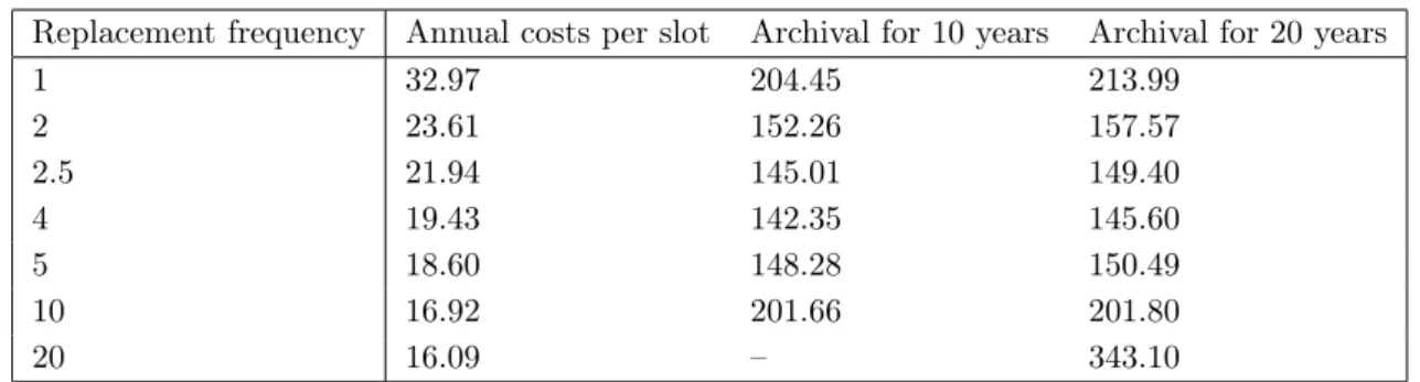
Replacement frequency Annual costs per slot Archival for 10 years Archival for 20 years

1 32.97 204.45 213.99

2 23.61 152.26 157.57

2.5 21.94 145.01 149.40

4 19.43 142.35 145.60

5 18.60 148.28 150.49

10 16.92 201.66 201.80

20 16.09 – 343.10

Table 6. Cost prediction for long-term archival of 2.5 TB of data in the DKRZ tape archive

Processor Memory Network Storage

Re-computation of results - - - +

Deduplication - - - 0 +

Compression (client side) - 0 + ++

Compression (server side) - 0 0 ++

User education + + + +

Table 7. Benefits and penalties of different concepts for data reduction (+ benefits; - penalties)

costs of 1,000,000e is added to support the libraries’ basic hardware and software. The LTO’s annual capacity increase of 32 % is a bit lower than the one of disks. Costs for different update frequencies are shown in Table 6. It can be seen that an update interval between 2.5–5 years is much cheaper than other intervals. Note that storing data for ten years is just slightly cheaper than keeping it for 20 years, which is already as expensive as storing the data forever. This consideration shows that the previous storage model for the archive is a bit conservative; it budgets 30 % more than if data is migrated to newer generations every four years.

5. Concepts to Dam the Data Deluge

Several concepts to reduce the amount of stored data will be discussed in this section: re-computation of results, deduplication of identical data and file-system-based as well as application-specific compression. Additional non-technical approaches such as educating users to improve storage usage will be mentioned briefly.

5.1. Re-computation

Instead of storing all produced data, there are several approaches to analyze data in-situ. A drawback of in-situ analysis is the fact that it requires a careful definition of the analyses to conduct before the actual application is executed since post-mortem data analysis is impossible. Consequently, whenever a new analysis is to be performed, the computation has to be restarted. Even though this approach sounds counterintuitive, re-computation can be attractive if the costs for keeping data on the storage are substantially higher than the costs for re-computation.

Table 5 shows the costs for computation, storage and archival of simulations in the frame of the CMIP5 and HD(CP)2 _{projects. In both cases, the cost of computation is higher than}

the cost for archiving the data in 2009. As mentioned previously, however, computational power continues to improve faster than storage technology; due to the storage systems falling further behind – effectively making it more expensive to store data – the picture changes from 2015 on: • 2015: Archiving an HD(CP)2_{simulation result for one year costs 13.91ewhile the}

compu-tation only costs 9.51e. For CMIP5, the difference is even greater as archival costs 1.66e while computation costs 0.60e. Consequently, if the data is only accessed once (HD(CP)2₎

or twice (CMIP5) it is cheaper to not archive the data but to re-compute it on demand. • 2020: For HD(CP)2 _{it is possible to re-compute the data more than seven times; for}

CMIP5 archival becomes more cost-efficient when the data is accessed more than 13 times. • 2025: As the gap between computation and storage increases, re-computation stays feasible

until the data has to be accessed more than 43 (HD(CP)2_{) or 100 (CMIP5) times.}

This analysis only takes re-computations on the same supercomputer into account. If data is supposed to be archived for even longer periods of time, however, it might be necessary to re-compute the data on a future superre-computer. This can present more challenges than simply keeping the application’s source code. To exactly reproduce the application’s behavior and, con-sequently, data output, it is necessary to preserve the complete operating environment instead. This includes but is not limited to: the application, all used libraries (such as MPI, NetCDF, HDF, etc.) and even the operating system. There are basically two ways to achieve this:

1. Binary preservation: Preserving the compiled binary code would effectively make it impos-sible to execute the application on differing future architectures (such as different processor architectures) without resorting to emulating the old environment. Emulation usually has significant performance impacts, making this approach infeasible for this use case. However, performing re-computation on the same supercomputer appears feasible using this approach. 2. Source preservation: Preserving the source code of all involved components makes sure that all components can be compiled even on different hardware architectures that might be available in the future. Consequently, even the exact compiler version would have to be preserved. However, even minute details such as changing behavior of different processors could lead to differing results.

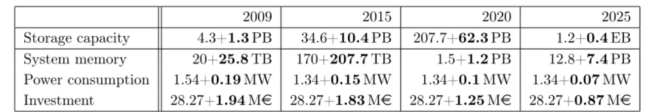
2009 2015 2020 2025 Storage capacity 5.6+1.68PB 45+13.5PB 270+81PB 1.6+0.48EB System memory 20+33.6TB 170+270TB 1.5+1.62PB 12.8+9.6PB Power consumption 1.6+0.24MW 1.4+0.20MW 1.4+0.14MW 1.4+0.09MW Investment 30+2.52Me 30+2.38Me 30+1.62Me 30+1.13Me

Table 8. Impact of deduplication for selected DKRZ systems (changes due to deduplication are marked in bold)

5.2. Deduplication

Deduplication works on the principle that data is split up into (possibly variably-sized) blocks and that each unique block of data is stored only once [23]. Instead of storing duplicate data, a reference to the original block is created for each repeated occurrence. Our previously conducted study for HPC data already showed great potential for data savings, allowing 20–30 % of redun-dant data to be eliminated on average [21]. To determine the potential savings, we independently scanned 12 sets of directories with a total amount of data of more than 1 PB. Deduplication was only applied within each set and not across the complete amount of data. We used a tool comput-ing the hashes of data to determine the deduplication potential; instead of the traditional static chunking method, content-defined chunking has been used. As mentioned previously, 20–30 % of data could be deduplicated on average; using full-file deduplication, it was still possible to reach savings of 5–10 %. Among the most interesting findings were the facts that between 3–9 % of the data consisted of zeros and that the top 5 % of chunks accounted for 35 % of the whole data set. Even though deduplication offers significant space savings, it also has its downsides: It can be very expensive in terms of memory overhead. For every 1 TB of deduplicated data, approximately 5–20 GB of storage are required to store the matching deduplication tables. The size of these tables heavily depends on the chosen block size. Enterprise deduplication solutions usually use block sizes between 4 KB and 16 KB to achieve high deduplication rates; we have settled on a block size of 8 KB for our following analysis. Using the SHA256 hash function (256 bits = 32 bytes) and 8 KB file system blocks (using 8 byte offsets) results in an overhead of at least 5 GB per 1 TB as shown in Equation (5.1). Additional data structure overhead will likely increase this number even further; consequently, we will assume an additional overhead of 8 bytes per hash, pushing the memory requirements to 6 GB of main memory per TB of storage. While it would be possible to increase the block size to reduce the overhead caused by the deduplication tables, this would also decrease the deduplication’s effectiveness.

The deduplication tables store references between the hashes and the actual data blocks within the file system. To enable efficient online deduplication, these tables have to be kept in main memory because potential duplicates have to be looked up for each write operation.

1 TB_÷8 KB = 125,000,000

125,000,000·(32 B + 8 B) = 5 GB (0.5 %) (5.1)

2009 2015 2020 2025 Storage capacity 4.3+1.3PB 34.6+10.4PB 207.7+62.3PB 1.2+0.4EB System memory 20+25.8TB 170+207.7TB 1.5+1.2PB 12.8+7.4PB Power consumption 1.54+0.19MW 1.34+0.15MW 1.34+0.1MW 1.34+0.07MW Investment 28.27+1.94Me 28.27+1.83Me 28.27+1.25Me 28.27+0.87Me

Table 9. Deduplication impact if storage capacity is preserved on selected DKRZ systems (changes due to deduplication are marked inbold)

established value of 6 GB main memory per 1 TB of storage space. According to our previous study [21], we have used an optimistic estimation of 30 % for the increase in storage capacity due to deduplication. Based on [17, page 165], the power consumption overhead for the additional system memory has been calculated using an estimated 9 % of the overall power distribution. The investment costs for the system memory have been estimated using data from [3, page 49] for main memory prices in 2020. Note that additional processor time and energy costs for computing the hash and the additional randomization of data accesses are not covered in this analysis.

For data center operators and vendors, it can also be interesting to quantify the potential benefits of a deduplication system. Therefore, Table 9 shows the characteristics of selected sys-tems where the goal is to preserve the overall storage capacity. As can be seen from this analysis, the investment costs and power consumption would be larger for the 2009 and 2015 systems. Therefore, with only 30 % deduplication rate the average 8 KB blocks would imply too much overhead and costs. However, investment costs for the 2020 and 2025 systems are slightly lower and so would be the power consumption of the 2025 system.

Discussion Overall, deduplication can be used to significantly increase storage capacity by removing duplicate data blocks. However, the presented configuration using 8 KB blocks has an overall negative impact on the cost of the storage system. There are several ways to remedy this: • Using larger block sizes can significantly reduce the memory overhead caused by the dedu-plication tables. When using 8 KB blocks, 0.6 % of the storage capacity have to be added as additional main memory; increasing the block size to 16 KB or 32 KB can lower this to 0.3 % or 0.15 %, respectively. However, the impact of larger block sizes on the deduplication ratio has to be considered and analyzed further.

• A cheaper alternative would be to use full-file deduplication only. This approach would not save any actual I/O bandwidth because the file has to be written completely before its hash can be determined. Additionally, the deduplication rate would be lower.

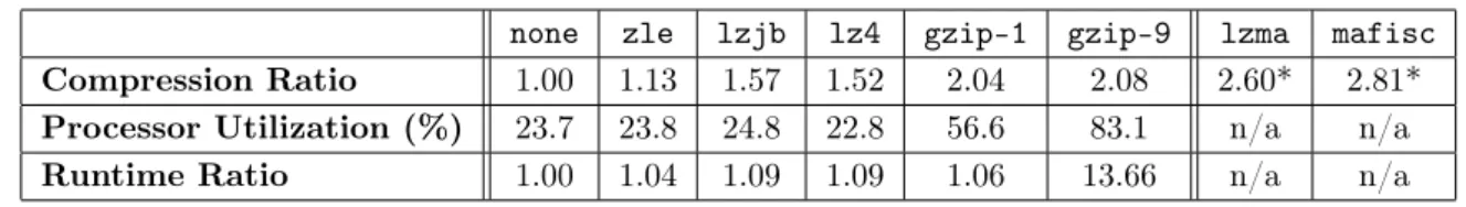
none zle lzjb lz4 gzip-1 gzip-9 lzma mafisc

Compression Ratio 1.00 1.13 1.57 1.52 2.04 2.08 2.60* 2.81*

Processor Utilization (%) 23.7 23.8 24.8 22.8 56.6 83.1 n/a n/a

Runtime Ratio 1.00 1.04 1.09 1.09 1.06 13.66 n/a n/a

Table 10.Comparison of different compression algorithms (lzma andmafisc’s ratios are estimated)

5.3. Compression

Similar to deduplication, compression can be used to reduce the amount of data that has to be stored on the storage system. While deduplication can only be employed meaningfully on the storage servers, compression can be used on both the clients and the servers.

On the one hand, processor overhead caused by client-side compression might negatively influence applications; however, data can be compressed before being sent to the servers, possibly reducing the required network bandwidth. On the other hand, server-side compression can be completely transparent to the clients. Independently of the location, compression uses additional processor time, which might require more powerful processors; this, in turn, can increase the overall power consumption.

In our previous HPC compression study, we leveraged Lustre 2.5 with its ZFS back-end file system to achieve transparent file system level compression [6]. ZFS is a local file system that offers a rich set of advanced features. Among others, it provides advanced storage device manage-ment, data integrity, as well as transparent compression and deduplication. It supports several compression algorithms: zero-length encoding zle, lzjb (a modified version of LZRW1 [31]), lz4 [32] andgzip(a variation of LZ77 [33]). We evaluated all of them using a scientific data set containing data from the Max Planck Institute Ocean Model (MPI-OM). The data set consists of around 73 % binary data and 27 % NetCDF data [24]. We have not considered decompression yet, because the evaluated compression algorithms are expected to have higher overheads when compressing than when decompressing.

Table 10 shows a comparison of the most interesting compression algorithms supported by ZFS; the data set was copied from an uncompressed ZFS pool into another separate compressed ZFS pool and processor utilization as well as runtime were recorded. All compression algorithms increase the runtime ratio only slightly; however, while zle, lzjb and lz4 only use negligible amounts of processor time, gzip adds significant overhead. gzip additionally allows the com-pression level (1–9) to be specified; higher comcom-pression levels do not significantly improve the compression ratio but increase the runtime and processor utilization considerably. Consequently, we choselz4 and gzip-1for further analysis.

Comp. Runtime Power Energy

Algorithm Ratio Ratio Ratio

none 1.0 1.0 1.0

lz4 0.92 1.01 0.93

gzip-1 0.92 1.10 1.01

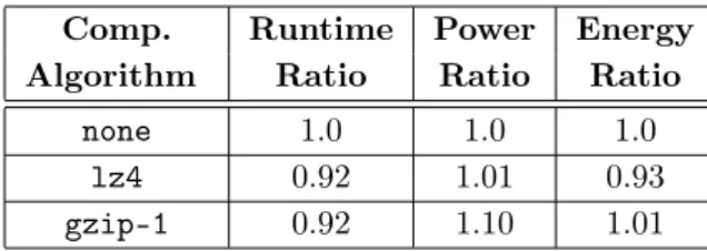
Table 11.Power and energy consumption of parallel I/O benchmark using selected compression algorithms

2009 2015 2020 2025

Storage capacity 5.6+2.8PB 45+22.5PB 270+135PB 1.6+0.8EB Power consumption 1.6+0.025MW 1.4+0.025MW 1.4+0.025MW 1.4+0.025MW

Table 12.Impact of server-side lz4 compression for selected DKRZ systems (changes are marked inbold)

the energy consumption was decreased for lz4 because of the lower runtime combined with the negligible increase in power consumption. For gzip-1, the total energy consumption increased by 1 % due to the higher power consumption caused by the elevated processor utilization.

An overview of the DKRZ’s supercomputers from 2009 to 2025 and the influence that large-scale compression of the complete storage system would have is shown in Table 12. The only important characteristics are storage capacity and power consumption; their base values have been taken from Table 1. We ignore the archive because compression is already enabled by default for the tape systems. The amount of additional storage has been calculated using a compression ratio of 1.5 forlz4as shown in Table 10. The power consumption overhead has been pessimistically estimated to be at most 10 % of the storage system’s overall power consumption; these numbers are based on Table 11, assuming a worst-case runtime ratio of 1.0. Additionally, we assume that it is not necessary to purchase more powerful processors; consequently, there is no negative influence on the investment cost.

Discussion Overall, compression can significantly increase the available storage capacity with only negligible overhead. In contrast to approaches like deduplication, no additional hardware investments are necessary. Coupled with the marginal increase in the storage system’s power consumption, the overall effect is very beneficial.

6. Summary, Conclusions and Future Work

To estimate current and future expenses, firstly, we predicted potential characteristics of the next DKRZ supercomputers, discussing the hardware trend in relation to Exascale studies. While the computational power grows by 20x every generation, the storage capacity increase of 6x lags behind. Applying the developed cost model to two typical experiment runs, the approximate costs for computation, storage and archival are quantified. Moreover, we discussed cost models for long-term archival under the trend of increasing areal densities and performance. It becomes apparent that keeping data available – yet not using it – is dominating the costs and its fraction will increase significantly with the next systems.

We compare concepts to handle the increasing storage costs: For low numbers of accesses, re-computation of data is promising, but requires concepts to guarantee reproducibility of the results. Deduplication may be beneficial but is not really promising in its current form. However, it is a tool to identify inefficient use of storage space which could be mitigated by proper user education. By improving performance and capacity, server-side compression bears the potential to reduce the TCO significantly; it is especially useful for data that is not compressed by the scientists explicitly. An advantage of client-side compression is the chance for achieving better compression ratios by taking the data format into account. Of these concepts, lossy compression achieves the best compression ratio but forces the user to define the required accuracy.

In the future, we plan to elaborate the cost model and use it to make decisions for new applications, as it is a potential source of future cost savings. We also continue our work on tools to analyze the users’ workflow in order to identify suboptimal usage scenarios and mitigate their impact. Finally, we will explore the benefits of adaptive compression and interfaces that enable more intelligent compression by providing semantical information. We believe that a proper analysis of all cost factors of an HPC system and the usage characteristics allows for an optimal configuration of the system and thus a maximum cost-benefit ratio.

Acknowledgment: We thank Carsten Beyer, Joachim Biercamp, Hinrich Reichardt, Michael Probst, Panagiotis Adamidis, Stefanie Legutke for providing valuable input and Michaela Zimmer and Konstantinos Chasapis for their reviews.

References

1. CMIP5 – Overview. http://cmip-pcmdi.llnl.gov/cmip5/. Last accessed: 2014-06. 2. IBM researchers make 12-atom magnetic memory bit. http://www.bbc.com/news/

technology-16543497, 2012. Last accessed: 2014-06.

3. Technical Challenges of Exascale Computing. Technical report, The MITRE Corporation, April 2013.http://institute.lanl.gov/resilience/docs/JSR-12-310-Challenges_of_ exascaleFINAL.pdf.

4. Allison H. Baker, Haiying Xu, John M. Dennis, Michael N. Levy, Doug Nychka, and Sheri A. Mickelson. A Methodology for Evaluating the Impact of Data Compression on Climate Sim-ulation Data. ACM Symposium on High-Performance Parallel and Distributed Computing, 2014, to appear.

6. Konstantinos Chasapis, Manuel Dolz, Michael Kuhn, and Thomas Ludwig. Evaluating Power-Performace Benefits of Data Compression in HPC Storage Servers. In Steffen Fries and Petre Dini, editors,IARIA Conference, pages 29–34. IARIA XPS Press, 04 2014. 7. Matthew L. Curry, H. Lee Ward, Gary Grider, Jill Gemmill, Jay Harris, and David Martinez.

Power Use of Disk Subsystems in Supercomputers. In Proceedings of the Sixth Workshop on Parallel Data Storage, PDSW ’11, pages 49–54, New York, NY, USA, 2011. ACM.

8. Department of Energy. Exascale Strategy – Report to Congress. Technical report, United States Department of Energy, June 2013. http://assets.fiercemarkets.net/public/ sites/govit/perera_fgit_foia_doe_exascale%20report.pdf.

9. Jack Dongarra. Impact of Architecture and Technology for Extreme Scale on Software and Algorithm Design. presentation, 2010.

10. Giovanni Erbacci, Vincent Bergeaud Francois Bodin, Alberto Pasanisi, Simon McIntosh-Smith, Thomas Ludwig, Franck Cappello, Carlo Cavazzoni, and Marie-Christine Sawley. European Exascale Software Initiative 2 Deliverable D5.1 – WP5 First Intermediate Report – Cross Cutting Issues Working Groups. http://www.eesi-project.eu/modules/download_ pictures/dlc.php?file=343&id=1389118661&sid=233, 2013.

11. Richard Freitas, Joseph Slember, Wayne Sawdon, and Lawrence Chiu. GPFS scans 10 billion files in 43 minutes. IBM Advanced Storage Laborator. IBM Almaden Research Center. San Jose, CA, 95120, 2011.

12. Serge Goldstein. DataSpace: A Model for Long-Term Preservation and Dissemination of Research Data. University of Massachusetts and New England Area Librarian e-Science Symposium, presentation, 2011.

13. Damien Hardy, Isidoros Sideris, Ali Saidi, and Yiannakis Sazeides. EETCO: A tool to estimate and explore the implications of datacenter design choices on the tco and the en-vironmental impact. In Workshop on Energy-efficient Computing for a Sustainable World, 2011.

14. Nathanael Hübbe and Julian Kunkel. Reducing the HPC-Datastorage Footprint with MAFISC – Multidimensional Adaptive Filtering Improved Scientific data Compression. In Computer Science - Research and Development, Hamburg, Berlin, Heidelberg, 2012. Execu-tive Committee, Springer.

15. Nathanael Hübbe, Al Wegener, Julian Kunkel, Yi Ling, and Thomas Ludwig. Evaluat-ing Lossy Compression on Climate Data. In Julian Martin Kunkel, Thomas Ludwig, and Hans Werner Meuer, editors, Supercomputing, number 7905 in Lecture Notes in Computer Science, pages 343–356, Berlin, Heidelberg, 06 2013. Springer.

16. Intel. Intel Solid State Drive DC S3700 Series – Product Specification, March 2014.

18. Julian Kunkel, Olga Mordvinova, Michael Kuhn, and Thomas Ludwig. Collecting Energy Consumption of Scientific Data. Computer Science - Research and Development, pages 1–9, 2010.

19. S. Lakshminarasimhan, N. Shah, S. Ethier, S.H. Ku, CS Chang, S. Klasky, R. Latham, R. Ross, and N.F. Samatova. Isabela for effective in situ compression of scientific data. Concurrency and Computation: Practice and Experience, 2012.

20. P. Lindstrom and M. Isenburg. Fast and efficient compression of floating-point data. Visu-alization and Computer Graphics, IEEE Transactions on, 12(5):1245–1250, Sept 2006. 21. Dirk Meister, Jürgen Kaiser, Andre Brinkmann, Michael Kuhn, Julian Kunkel, and Toni

Cortes. A Study on Data Deduplication in HPC Storage Systems. In Proceedings of the ACM/IEEE Conference on High Performance Computing (SC), 11 2012.

22. Chris Mellor. Spin that disk drive forecast, Gartner: Watch those desktop units dive. http: //www.theregister.co.uk/2014/03/31/gartner_disk_drive_forecast/, 2014.

23. Dutch T. Meyer and William J. Bolosky. A study of practical deduplication. InProceedings of the 9th USENIX Conference on File and Stroage Technologies, FAST’11, pages 1–1, Berkeley, CA, USA, 2011. USENIX Association.

24. Russ Rew and Glenn Davis. Data Management: NetCDF: an Interface for Scientific Data Access. IEEE Computer Graphics and Applications, (10-4):76–82, 1990.

25. The HD(CP)2 _{Project. HD(CP)}2_{. http://hdcp2.eu/. Last accessed: 2014-06.}

26. The TOP500 Editors. TOP500. http://www.top500.org/, 06 2013. Last accessed: 2013-06. 27. Thomas Ludwig. The Costs of HPC-Based Science in the Exascale Era. Invited talk at the

Supercomputing Conference SC12, Salt Lake City, 2012.

28. Thomas Ludwig and Albert Reuther and Amy Apon. Cost-Benefit Quantification for HPC: An Inevitable Challenge. Birds of a Feather session at the Supercomputing Conference SC13, Denver, 2013.

29. Wikipedia. Festplattenlaufwerk – Geschwindigkeit. http://de.wikipedia.org/wiki/ Festplattenlaufwerk#Geschwindigkeit, 02 2013. Last accessed: 2013-02.

30. Wikipedia. Mark Kryder – Kryder’s Law. http://en.wikipedia.org/wiki/Mark_Kryder# Kryder.27s_Law, 02 2013. Last accessed: 2013-02.

31. R.N. Williams. An extremely fast Ziv-Lempel data compression algorithm. In Data Com-pression Conference, 1991. DCC ’91., pages 362–371, Apr 1991.

32. Yann Collet. LZ4 Explained. http://fastcompression.blogspot.com/2011/05/ lz4-explained.html, 2008. Last accessed: 2013-12.

33. J. Ziv and A. Lempel. A universal algorithm for sequential data compression. Information Theory, IEEE Transactions on, 23(3):337–343, May 1977.