466
Rev. bus. manag., São Paulo, Vol. 16, No. 52, pp. 466-483, Jul./Sept. 2014
REVISTA BRASILEIRA DE GESTÃO DE NEGÓCIOS ISSN 1806-4892
REVIEw Of BuSINESS MANAGEMENT © FECAP
DOI: 10.7819/rbgn.v16i52.1555
Subject Area: Accounting And Controlling
RBGN
Accounting Fraud: an estimation of detection probability
Fraudes Contábeis: uma estimativa da probabilidade de detecção
Fraudes contables: una estimación de la probabilidad de detección
Artur Filipe Ewald Wuerges1 José Alonso Borba2
Received on February 20, 2013 / Approved on October 1, 2014 Responsible Editor: Ivam Ricardo Peleias, Dr.
Evaluation Process: Double Blind Review
1. Master in Management from Federal University of Santa Catarina (UFSC). [[email protected]] 2. Doctor in Accounting from University of São Paulo (USP). [[email protected]]
Authors’ address: Rua Major Antônio Cardoso, 590, CEP: 97900-000 – Cerro Largo – RS – Brazil
ABSTRACT
Financial statement fraud (FSF) is costly for investors and can damage the credibility of the audit profession. To prevent and detect fraud, it is helpful to know its causes. The binary choice models (e.g. logit and probit) commonly used in the extant literature, however, fail to account for undetected cases of fraud and thus present unreliable hypotheses tests. Using a sample of 118 companies accused of fraud by the Securities and Exchange Commission (SEC), we estimated a logit model that corrects the problems arising from undetected frauds in U.S. companies. To avoid multicollinearity problems, we extracted seven factors from 28 variables using the principal factors method. Our results indicate that only 1.43 percent of the instances of FSF were publicized by the SEC. Of the six significant variables included in the traditional, uncorrected logit model, three were found to be actually non-significant in the corrected model. The likelihood of FSF is 5.12
times higher when the firm’s auditor issues an adverse or qualified report.
Keywords: Accounting fraud. AAER. Misclassification. Logit. Factor analysis.
RESUMO
Para evitar problemas de multicolinearidade, extraímos sete fatores a partir de 28 variáveis, usando o método dos componentes principais. Nossos resultados indicam que apenas 1,43% dos casos de FDF foram divulgados pela SEC. Das sete variáveis significativas incluídas em um modelo logit tradicional e não corrigido, três na realidade não foram consideradas significativas em um modelo corrigido. A probabilidade de FDF é 5,12 vezes maior quando o auditor da empresa emite um parecer adverso ou com ressalvas.
Palavras-chave: Fraude contábil. AAER. Erros de classificação. Logit. Análise fatorial.
RESUMEN
El fraude en los estados financieros (FEF) es costoso para los inversionistas y pueden minar la credibilidad de los auditores. A fin de prevenir y detectar el fraude, es útil conocer sus causas. Sin embargo, los modelos de elección binaria (logit y probit, por ejemplo) a menudo utilizados en la literatura, no tienen en cuenta los casos de fraudes detectados y consecuentemente presentan pruebas de hipótesis poco fiables. Utilizando una muestra de 118 compañías acusadas de fraude por la Comisión de Bolsa y Valores de EE.UU. (Securities and Exchange Commission, SEC), hemos estimado un modelo logit que corrige los problemas derivados de los fraudes no detectados en las compañías estadounidenses. Para evitar problemas de multicolinealidad, hemos extraído siete factores de 28 variables, utilizando el método de componentes principales. Nuestros resultados indican que sólo el 1,43% de los casos de FEF se han dado a conocer por la SEC. De las siete variables significativas incluidas en un modelo logit tradicional y no corregido, tres en efecto no fueron consideradas significativas en un modelo corregido. La probabilidad de FEF es 5,12 veces mayor cuando el auditor de la compañía emite una opinión adversa o con reservas.
Palabras clave: Fraude contable. AAER. Errores de clasificación. Logit. Análisis factorial.
1 INTRODUCTION
In modern corporations, it is common to adopt a structure that separates ownership from management. Although the shareholders have voting rights, the daily management is actually done by professional executives appointed by the board of directors (that are themselves elected by the shareholders). This situation opens the way for conflicts of interest: The decisions taken by executives are not always the ones the shareholders would take if they were managing the company (JENSEN; MECKLING, 1976). For example, the CEO might buy a first class flight ticket, whereas a shareholder would probably prefer to pay a cheaper airfare.
This misalignment of interests will usually incur in agency costs for the company. Some of these agency costs are monitoring costs: the shareholders are willing to invest in the development of a monitoring system capable of avoiding abuse by managers. The financial statements, produced in accordance with some financial reporting standards (e.g. IFRS), are part of this monitoring system. Even though they are a cost (ultimately paid by the shareholders), they allow investors access to information about the quality of the management of the company. In order to assure investors that adequate reporting standards were actually followed, the company will usually engage an independent auditor. In fact, financial statement users commonly rely on auditors to prevent and detect financial statement fraud and errors (BEST; BUCKBY; TAN, 2001; LEE; GLOECK; PALANIAPPAN, 2007), although “it is management’s responsibility to design and implement programs and controls to prevent, deter, and detect fraud.” (AICPA, 2002, p. 169)
468
Rev. bus. manag., São Paulo, Vol. 16, No. 52, pp. 466-483, Jul./Sept. 2014 Artur Filipe Ewald Wuerges / José Alonso Borba
last instance paid by the stockholders when the stock prices plummet after the announcement of fraud charges by the Securities and Exchange Commission (GERETY; LEHN, 1997). Some big companies now associated to fraud in the U.S. are Adelphia, Enron, Tyco and WorldCom. This surge of frauds led to a legislative reform known as Sarbanes-Oxley Act (SOX), which established new standards of transparency for public companies. In spite of these measures, frauds still occur (even though their number apparently decreased after 2002), and therefore are still a relevant theme for academic research.
Failure to detect or prevent financial statement fraud can damage the reputation and the credibility of the audit profession (CHUI; PIKE, 2011). In fact, some argue that fraud is the Achilles heel of the audit profession, at least in part because risk-based auditing is predictable (JAMAL, 2008). Using past cases of fraud to build models to estimate the risk of fraud does not help auditors to become unpredictable, but may help them to understand the causes of financial statement fraud. Regression analysis (i.e. logit and probit models) allows the test of hypotheses about the influence of certain variables on the occurrence of fraud.
One of the problems of this approach is that there are cases of fraud that still have not been discovered, and some of them probably will never be. It is also possible that the SEC chooses to focus on high-profile fraud cases, and therefore some cases are actually detected to some degree, but not fully investigated and reported in AAERs. Finally, it is also possible that the commission suspects some financial statements are intentionally misstated but is unable to present evidence to support its suspicion. It would not be surprising, then, if just a small part of accounting frauds is discovered, fully investigated and disclosed to the public. In a regression analysis, this generates misclassification problems in the dependent variable. There are companies incorrectly excluded from the list of cases of fraud. These errors harm the model, biasing the estimates of the parameters. It is therefore possible that the hypotheses tests are affected, making the conclusions misleading.
Hausman, Abrevaya, and Scott-Morton (1998) developed a method capable of minimizing this problem and also of estimating the probability that a case of fraud is not discovered. This study examines the results of such method applied to financial statement fraud, to assess whether its results are different from the ones obtained with an uncorrected logit model.
This paper has three objectives. Our first objective was to estimate the percentage of unreported frauds in U.S. companies. Doing so, we can analyze how effective the SEC is in detecting and repressing financial statement fraud. Our second objective was to check if the results obtained using a traditional logit model are qualitatively different from those obtained using a logit model with the misclassification parameter. Our last objective was to obtain reliable hypotheses tests regarding some variables that might be related to financial statement fraud.
2 THEORETICAL BACKGROUND AND VARIABLES
Fraud, in a broad sense, is defined as the conscious distortion of truth or concealment of material fact with the objective of inducing other people to act to the detriment of their own interests (PEDNEAULT, 2009). When an executive intentionally distort financial statements, he or she is also committing fraud. There is a conscious act that induces other people to act to the detriment of their own interests, like paying a high price for common stock that is actually worth much less. These cases are known as financial statement fraud (ALBRECHT, W. S. et al., 2009).
It is important to add that financial statement frauds are perpetrated by violating Generally Accepted Accounting Principles (GAAP). If there is no violation of GAAP, then it is a case of earnings management, which is also harmful to investors but resorts only to legal means (DECHOW; SKINNER, 2000).
variables that explain the occurrence of fraud. There are concepts and theories that explain white-collar crime and some of them can also be employed as a starting point to understand the causes of accounting fraud, thereby serving as a guide for the selection and organization of independent variables. It is common to use the fraud triangle, originally proposed by Donald R. Cressey to explain the occurrence of white-collar crime. This author believes that these crimes occur when three factors are present: pressure (financial need), opportunity and rationalization. In the early 1980’s, Steve Albrecht adapted this theory to the study of financial statement fraud (CHOO; TAN, 2007). We classify the variables used in this study in these three groups.
It must be noted that, when estimating a logit model, an observation is dropped if there is a value missing for any variable. To avoid working with a small sample, we excluded all the variables with fewer than 20,000 observations. These variables were collected, but are not used or mentioned in this paper.
2.1 Pressure
The pressure (financial need) is related to the situation of the company and its managers. It is expected that companies that have been unable to attain the expectations of the market are more susceptible to fraud, since the managers are under pressure to perform well. For this reason, indicators of performance and financial security can be used for fraud detection, in association with other evidence. Enron, for example, was a highly leveraged company that required its executives to obtain (and report) large profits in order to be able to pay interests and fulfill contractual bonds (CHOO; TAN, 2007).
To capture the elements of pressure in the model, we used several different indicators. One of them is the Altman’s Zscore (zscore), a proxy for risk of financial distress often used in financial statement fraud research (ALTMAN, 1968). We expect companies with higher Z scores to be in better financial position and therefore less likely to resort to fraud, although previous research
shows it is negatively related to the likelihood of fraud in Greek companies (KIRKOS; SPATHIS; MANOLOPOULOS, 2007; SPATHIS, 2002), but statistically unrelated to fraud in U.S. firms (ERICKSON; HANLON; MAYDEW, 2006; FANNING; COGGER, 1998; SUMMERS; SWEENEY, 1998). We also used several other variables that attempt to measure the companies’ ability to cover their liabilities, since companies that have trouble paying their debts (and therefore have financial problems) may recourse to FSF in order to obtain financial resources, either in the capital markets or through loans. One of these variables is the cash scaled by total assets (CASHTA), proposed by Gaganis (2009), who found it to be negatively related to fraud. We also adopted the cash change scaled by total assets (ΔCASHTA). Another variable related to liquidity is the current assets divided by current liabilities (CACL), also known as current ratio. A CACL
lower than 1 suggests that the company does not have enough assets readily available to pay its short term debt and therefore signals possible insolvency problems. We expect this variable and its change (ΔCACL) to be negatively related to fraud, although there are previous studies that found this variable to be statistically unrelated to FSF (BENEISH, 1999a; KIRKOS; SPATHIS; MANOLOPOULOS, 2007). Another variable is the working capital (i.e. current assets minus current liabilities) divided by total assets (WCTA), used by Beneish (1997, 1999a, 1999b), Fanning and Cogger (1998), Spathis (2002), Kirkos, Spathis, and Manolopoulos (2007), and Gaganis (2009). We expect this variable and its change (ΔWCTA) to be negatively related to fraud.
470
Rev. bus. manag., São Paulo, Vol. 16, No. 52, pp. 466-483, Jul./Sept. 2014 Artur Filipe Ewald Wuerges / José Alonso Borba
MAYDEW, 2006; ETTREDGE et al., 2008; JOHNSON; RYAN; TIAN, 2008; WANG, 2011). We also used the change in this variable (ΔTLTA). Very similar measures of leverage, used by Fanning and Cogger (1998), can be obtained by substituting total equity for total assets (TLTE and ΔTLTE). Another indicator of financial security is the ratio of sales to accounts receivables (SALAR), used by Summers and Sweeney (1998), Spathis (2002), Kirkos, Spathis, and Manolopoulos (2007), and Skousen and Wright (2008). We expect it to be negatively related to the likelihood of fraud. Kaminski, Wetzel, and Guan (2004) used yet another ratio for financial security, given by interest expenses divided by total liabilities (IETL).
Another variable that can be used is FATA, the ratio of fixed assets to total assets (KIRKOS; SPATHIS; MANOLOPOULOS, 2007). It is the fixed assets (e.g. equipment and factories) that generate revenues for the company, and therefore we expect that companies with a large value invested in fixed assets are less likely to engage in fraud, since they are in better position to generate real revenue in the future. According to Kirkos, Spathis, and Manolopoulos, FATA
is unrelated to fraud in Greek companies. We also used the change in this variable (ΔFATA). Another variable, proposed by Gaganis (2009) and negatively correlated to FATA, is obtained dividing the current assets by the total assets (CATA). Its change was also used in this study (ΔCATA). Gaganis found CATA to be significantly lower in companies involved in FSF.
Some authors suggest using the cost of goods sold divided by the sales (KAMINSKI; WETZEL; GUAN, 2004). We expect this variable (COGSAL) and its change (ΔCOGSAL) to be positively related to the likelihood of fraud, since an increase in the cost of goods sold can signal a decrease in the company’s ability to compete.
Spathis (2002) and Kirkos, Spathis, and Manolopoulos (2007) used in their models a variable obtained by dividing the net profit by the sales. We used EBIT (earnings before interest and taxes) divided by sales (EBITSAL)
as a predictor of FSF. The rationale behind this variable is that a decrease in profitability creates pressure that might cause the company to recourse to fraud. A similar variable is EBIT scaled by total assets (EBITTA). We also used the change in this variable (ΔEBITTA). Another measure of profitability is the net profit scaled by total assets (ROA) and its change (ΔROA). While building variables such as EBITTA and ROA, it should be noted that variables obtained from the income statement (such as net profit or EBIT) are attributed to the entire period, whereas variables obtained from the balance sheet (such as total assets) are attributed to a given point in time. To make the denominator comparable to the numerator, we used the average total assets in the relevant period of time to generate the variables
EBITTA and ROA, as well as their changes. The extant literature also presents variables based in the inventory value. The presence of too much inventory might signal that the company is unable to sustain the expected sales levels or is simply inefficient. Fanning and Cogger (1998) and Gaganis (2009), using inventory divided by sales (INVSAL), found evidence supporting this hypothesis. On the other hand, in Greek companies, this variable seems to be statistically not significant (KIRKOS; SPATHIS; MANOLOPOULOS, 2007; SPATHIS, 2002). Summers and Sweeney (1998) argue that financial statement fraud is related to the growth in inventory (ΔINVSAL). We use this variable because some industries might have usually high inventory levels. Finally, some authors used inventory divided by total assets (INVTA), but found it to be statistically not significant (FANNING; COGGER, 1998; GAGANIS, 2009; KIRKOS; SPATHIS; MANOLOPOULOS, 2007).
2.2 Opportunity
actively seek means to bypass the institutional mechanism created to repress fraud. This means that even when opportunity is not present, in some cases managers will create them. Pressure for success generates opportunities for criminal behavior. The managers of Cendant, a company charged with fraud, kept a yearly spreadsheet with “opportunities” available to inflate operational revenue, and also listed the values that should be obtained in each of these opportunities.
In our model, the variable that represents the opportunity to fraud is a dummy for auditor change (ETTREDGE et al., 2008; FANNING; COGGER, 1998; SKOUSEN; WRIGHT, 2008), here abbreviated as AUDCH. According to Summers and Sweeney (1998), it is possible that a company that engages in fraud will change its auditor to diminish the likelihood of getting caught.
2.3 Rationalization
Managers involved in fraud (and white-collar criminals in general) “‘adjust’ the symbolic construction of their behavior to conform to generalized social expectations,” in a process often referred to as rationalization (COLEMAN, 1987, p. 410). They might, for instance, claim that their actions were necessary for the company to survive and avoid layoffs. Or, in highly competitive industries, managers might contend that fraudulent acts are widespread, effectively constructing them as something natural and expected.
For Skousen and Wright (2008), the accruals level is representative of the management’s way of making decisions about financial statements. When earnings management is seen as normal, more serious actions might be the next step. Since excessive use of accruals often motivate modified audit reports (FRANCIS; KRISHNAN, 1999), we used a dummy variable (UQUAL) that is equal to 1 if the audit report presents an unqualified (clean) opinion. The opinion is unqualified when the financial statements reflect no unresolvable restrictions and the auditor has no significant exceptions. Unqualified opinions
with additional language are coded as 0, since they might reflect excessive use of accruals. In any other case (e.g. qualified or adverse opinion), the variable is equal to 0.
2.4 Similar studies
There are several papers that used probit and logit models to estimate the likelihood of FSF or identify the variables that influence this likelihood. Some of them also used AAERs to build the dependent variable (ABBOTT; PARK; PARKER, 2000; BRAZEL; JONES; ZIMBELMAN, 2009; CRUTCHLEY; JENSEN, M. R. H.; MARSHALL, 2007; ERICKSON; HANLON; MAYDEW, 2006; ETTREDGE et al., 2008; JOHNSON; RYAN; TIAN, 2008; LENNOX; PITTMAN, 2010; MILLER, 2006; SKOUSEN; WRIGHT, 2008; PERSONS, 1995). Other authors used the cases of fraud publicized by the press, either alone or jointly with AAERs (BEASLEY, 1996; BENEISH, 1997; LEE; INGRAM; HOWARD, 1999; SUMMERS; SWEENEY, 1998).
Articles using probit and logit often aim at checking the impact of a given variable on the occurrence of fraud. Erickson, Hanlon, and Maydew (2006), for example, studied the effect of stock option on fraud. The results of this article indicate that, contrary to what is often believed, there is no consistent evidence that stock-based incentives contribute to the occurrence of accounting fraud. These results were confirmed by the papers of Gerety and Lehn (1997) and Crutchley, Jensen, and Marshall (2007), but not by Erickson, Hanlon, and Maydew (2004). More recently, Feng et al. (2011) found evidence supporting the hypothesis that CFOs get involved in fraud because they succumb to pressure from CEOs, and not because they want to increase their income from equity incentives.
472
Rev. bus. manag., São Paulo, Vol. 16, No. 52, pp. 466-483, Jul./Sept. 2014 Artur Filipe Ewald Wuerges / José Alonso Borba
which the probability of fraud and the probability of fraud detection are estimated separately. The model used by Wang requires the identification of a set of variables that influence the likelihood of fraud detection. Our paper, on the other hand, estimated the unconditional likelihood of fraud detection (without the use of an additional set of independent variables). Some papers used artificial intelligence techniques to detect frauds. It is common to use neural networks for this purpose (CHOI; GREEN, 1997; FANNING; COGGER, 1998; OGUT et al., 2009). Some studies employed fuzzy logic (DESHMUKH; TALLURU, 1998), whereas others adopted hybrid methods like fuzzy neural networks (LIN; HWANG; BECKER, 2003). At last, there are articles that used several different fraud detection methods with the intent of comparing them (KIRKOS; SPATHIS; MANOLOPOULOS, 2007; GAGANIS, 2009).
One of the shortcomings of studies using artificial intelligence is the difficulty in testing hypotheses. It is not possible, for example, to test whether the likelihood of fraud is related to executive compensation. On the other hand, several studies concluded that artificial intelligence methods can identify the occurrence of fraud with higher accuracy when compared to probit and logit models (LIN; HWANG; BECKER, 2003; OGUT et al., 2009). The choice of tools depends on the objectives of the researcher. In this paper, since our objective is to estimate the likelihood of a fraud being undetected and test the hypothesis that this likelihood is different from zero, we have chosen a logit model.
3 METHOD
This article presents an empirical model. The data regarding financial statements were obtained in Compustat. The following sections describe how the AAERs published by the SEC were used to identify the companies charged with fraud in the U.S. and explain the novel method used to estimate the likelihood of a fraud being not detected.
3.1 Data
The companies accused of FSF were identified by an analysis of the Accounting and Auditing Enforcement Releases published by the SEC from 1 January 1998 to 23 November 2010. All the reports were read in search of material misstatements.
If the company was accused of fraud, we carefully read the release to identify the first fraud year – that is, the first year in which a materially false statement was published. There was care in checking the fiscal years of the accused companies. Compustat adopts a simple rule: If the fiscal year ends between 1 January and 31 May, then it is considered as being the previous calendar year. For example, a statement closed as of 31 March 2000 is stored in the database as being of the year 1999. Therefore, if a fraud was first identified in this statement, then the first fraud year is 1999. In other words, we made an effort to match the list of frauds and their years to the data provided by Compustat.
We removed all the occurrences of violation of the Foreign Corrupt Practices Act (FCPA) from the sample. The FCPA prohibits the practice of bribing foreign officials. Since bribery is illegal, the money used for such purposes does not pass through official accounting; the company might recourse to some kind of financial report violation in order to hide the destination of these resources. This can materially affect the financial statements of the company. Unfortunately, not every AAER issued because of FCPA violations states which financial statements were affected; sometimes, the amount channeled to bribes is negligible. Because of these problems, they were all removed from the sample.
company. Including stock options backdating in this study would just mix two different phenomena in the same dependent variable. Nevertheless, the practice of backdating stock options might also distort financial statements.
Due to technical limitations, we kept in the sample only companies listed in three stock exchanges (NYSE, NASDAQ and AMEX). This means that companies traded over the counter were excluded, as well as those with no data available in Compustat.
A financial statement fraud is usually discovered only several years after it has begun. It is therefore very difficult to have a meaningful sample of companies that issued falsified financial statements in recent years. Any attempt to do so would increase the number of cases of misclassification, since many more companies would be incorrectly labeled as honest. Therefore,
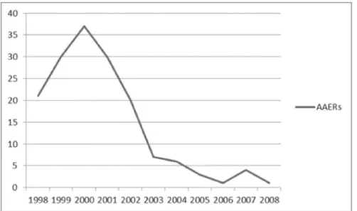
we also opted to remove from the sample those instances of fraud that occurred before 1998 and after 2002. As one can see in Figure 1, the number of frauds discovered after 2002 apparently fell abruptly. Instead of signaling a true reduction in the number of fraud cases, this fall more likely shows the SEC’s inability to report recent cases.
Financial companies – those with SIC (Standard Industrial Classification) codes from 6000 to 6999 – were also removed from the sample. The final sample contains 118 companies that fulfill all the requirements.
The models were not estimated only with the companies charged with fraud. The population of this study comprises all the companies with financial statements available in Compustat for the period ranging from the years 1998 to 2002. Companies with data for just some of these five years were included.
FIGURE 1 – AAERS issued between 1998 and 2008
Source: The authors
3.2 Factor analysis
Factor analysis is a multivariate technique that synthesizes the relationships observed in a set of interrelated variables, allowing the
474
Rev. bus. manag., São Paulo, Vol. 16, No. 52, pp. 466-483, Jul./Sept. 2014 Artur Filipe Ewald Wuerges / José Alonso Borba
(1)
where
Uma FDF costuma ser descoberta somente anos depois de começar. É difícil,
portanto, obter uma amostra significativa de empresas que tenham emitido
demonstrações financeiras falsificadas em exercícios recentes. Qualquer tentativa de
fazê-lo aumenta o número de casos de erros de classificação, visto que muito mais
empresa seriam inadequadamente classificadas como honestas. Assim, optamos também
por remover da amostra os casos de fraude ocorridos antes de 1998 e depois de 2002.
Como podemos verificar na Figura 1, o número de fraudes descobertas depois de 2002
aparentemente caiu de forma abrupta. Em vez de sinalizar uma verdadeira redução do
número de fraudes, essa queda mais provavelmente mostra a incapacidade da SEC de
denunciar casos recentes.
As empresas financeiras
–
as que possuem códigos de Classificação Industrial
Padrão (SIC) de 6000 a 6999
–
também foram removidas da amostra. A amostra final
contém 118 empresas que atendem a todos os requisitos.
Os modelos não foram estimados somente com as empresas acusadas de fraude. A
população deste estudo consiste em todas as empresas com demonstrações financeiras
disponíveis no Compustat no período de 1998 a 2002. As empesas com dados de apenas
alguns desses cinco anos foram incluídas.
FIGURA 1 – AAERSs EMITIDOS ENTRE 1998 E 2008
Fonte: Compilada pelos autores.
3.2 ANÁLISE FATORIAL
A análise fatorial é uma técnica multivariada que sintetiza a relação observada em
um conjunto de variáveis inter-relacionadas, permitindo a identificação de fatores
comuns. Segundo Jöreskog (1969), em uma análise fatorial com p
variáveis e k
fatores,
o modelo básico é:
(1)
em que
é um vetor de ordem p de variáveis observadas para observação i,
é
um vetor de ordem k
<
p de escores fatoriais latentes comuns para a observação i, e
é
um vetor de ordem p de escores únicos para observação i. Esses escores únicos podem
is a vector of order p of observed variables for observation i,
Uma FDF costuma ser descoberta somente anos depois de começar. É difícil,
portanto, obter uma amostra significativa de empresas que tenham emitido
demonstrações financeiras falsificadas em exercícios recentes. Qualquer tentativa de
fazê-lo aumenta o número de casos de erros de classificação, visto que muito mais
empresa seriam inadequadamente classificadas como honestas. Assim, optamos também
por remover da amostra os casos de fraude ocorridos antes de 1998 e depois de 2002.
Como podemos verificar na Figura 1, o número de fraudes descobertas depois de 2002
aparentemente caiu de forma abrupta. Em vez de sinalizar uma verdadeira redução do
número de fraudes, essa queda mais provavelmente mostra a incapacidade da SEC de
denunciar casos recentes.
As empresas financeiras
–
as que possuem códigos de Classificação Industrial
Padrão (SIC) de 6000 a 6999
–
também foram removidas da amostra. A amostra final
contém 118 empresas que atendem a todos os requisitos.
Os modelos não foram estimados somente com as empresas acusadas de fraude. A
população deste estudo consiste em todas as empresas com demonstrações financeiras
disponíveis no Compustat no período de 1998 a 2002. As empesas com dados de apenas
alguns desses cinco anos foram incluídas.
FIGURA 1 – AAERSs EMITIDOS ENTRE 1998 E 2008
Fonte: Compilada pelos autores.
3.2 ANÁLISE FATORIAL
A análise fatorial é uma técnica multivariada que sintetiza a relação observada em
um conjunto de variáveis inter-relacionadas, permitindo a identificação de fatores
comuns. Segundo Jöreskog (1969), em uma análise fatorial com p
variáveis e k
fatores,
o modelo básico é:
(1)
em que
é um vetor de ordem p de variáveis observadas para observação i,
é
um vetor de ordem k
<
p de escores fatoriais latentes comuns para a observação i, e
é
um vetor de ordem p de escores únicos para observação i. Esses escores únicos podem
is a vector of order k < p of latent common factor scores for the observation i, and
Uma FDF costuma ser descoberta somente anos depois de começar. É difícil,
portanto, obter uma amostra significativa de empresas que tenham emitido
demonstrações financeiras falsificadas em exercícios recentes. Qualquer tentativa de
fazê-lo aumenta o número de casos de erros de classificação, visto que muito mais
empresa seriam inadequadamente classificadas como honestas. Assim, optamos também
por remover da amostra os casos de fraude ocorridos antes de 1998 e depois de 2002.
Como podemos verificar na Figura 1, o número de fraudes descobertas depois de 2002
aparentemente caiu de forma abrupta. Em vez de sinalizar uma verdadeira redução do
número de fraudes, essa queda mais provavelmente mostra a incapacidade da SEC de
denunciar casos recentes.
As empresas financeiras
–
as que possuem códigos de Classificação Industrial
Padrão (SIC) de 6000 a 6999
–
também foram removidas da amostra. A amostra final
contém 118 empresas que atendem a todos os requisitos.
Os modelos não foram estimados somente com as empresas acusadas de fraude. A
população deste estudo consiste em todas as empresas com demonstrações financeiras
disponíveis no Compustat no período de 1998 a 2002. As empesas com dados de apenas
alguns desses cinco anos foram incluídas.
FIGURA 1 – AAERSs EMITIDOS ENTRE 1998 E 2008
Fonte: Compilada pelos autores.
3.2 ANÁLISE FATORIAL
A análise fatorial é uma técnica multivariada que sintetiza a relação observada em
um conjunto de variáveis inter-relacionadas, permitindo a identificação de fatores
comuns. Segundo Jöreskog (1969), em uma análise fatorial com p
variáveis e k
fatores,
o modelo básico é:
(1)
em que
é um vetor de ordem p de variáveis observadas para observação i,
é
um vetor de ordem k
<
p de escores fatoriais latentes comuns para a observação i, e
é
um vetor de ordem p de escores únicos para observação i. Esses escores únicos podem
unique scores for observation i. These unique is a vector of order p of scores can be seen as “error terms”: They represent the portion ofUma FDF costuma ser descoberta somente anos depois de começar. É difícil,
portanto, obter uma amostra significativa de empresas que tenham emitido
demonstrações financeiras falsificadas em exercícios recentes. Qualquer tentativa de
fazê-lo aumenta o número de casos de erros de classificação, visto que muito mais
empresa seriam inadequadamente classificadas como honestas. Assim, optamos também
por remover da amostra os casos de fraude ocorridos antes de 1998 e depois de 2002.
Como podemos verificar na Figura 1, o número de fraudes descobertas depois de 2002
aparentemente caiu de forma abrupta. Em vez de sinalizar uma verdadeira redução do
número de fraudes, essa queda mais provavelmente mostra a incapacidade da SEC de
denunciar casos recentes.
As empresas financeiras
–
as que possuem códigos de Classificação Industrial
Padrão (SIC) de 6000 a 6999
–
também foram removidas da amostra. A amostra final
contém 118 empresas que atendem a todos os requisitos.
Os modelos não foram estimados somente com as empresas acusadas de fraude. A
população deste estudo consiste em todas as empresas com demonstrações financeiras
disponíveis no Compustat no período de 1998 a 2002. As empesas com dados de apenas
alguns desses cinco anos foram incluídas.
FIGURA 1 – AAERSs EMITIDOS ENTRE 1998 E 2008
Fonte: Compilada pelos autores.
3.2 ANÁLISE FATORIAL
A análise fatorial é uma técnica multivariada que sintetiza a relação observada em
um conjunto de variáveis inter-relacionadas, permitindo a identificação de fatores
comuns. Segundo Jöreskog (1969), em uma análise fatorial com p
variáveis e k
fatores,
o modelo básico é:
(1)
em que
é um vetor de ordem p de variáveis observadas para observação i,
é
um vetor de ordem k
<
p de escores fatoriais latentes comuns para a observação i, e
é
um vetor de ordem p de escores únicos para observação i. Esses escores únicos podem
that cannot be explained by
Uma FDF costuma ser descoberta somente anos depois de começar. É difícil,
portanto, obter uma amostra significativa de empresas que tenham emitido
demonstrações financeiras falsificadas em exercícios recentes. Qualquer tentativa de
fazê-lo aumenta o número de casos de erros de classificação, visto que muito mais
empresa seriam inadequadamente classificadas como honestas. Assim, optamos também
por remover da amostra os casos de fraude ocorridos antes de 1998 e depois de 2002.
Como podemos verificar na Figura 1, o número de fraudes descobertas depois de 2002
aparentemente caiu de forma abrupta. Em vez de sinalizar uma verdadeira redução do
número de fraudes, essa queda mais provavelmente mostra a incapacidade da SEC de
denunciar casos recentes.
As empresas financeiras
–
as que possuem códigos de Classificação Industrial
Padrão (SIC) de 6000 a 6999
–
também foram removidas da amostra. A amostra final
contém 118 empresas que atendem a todos os requisitos.
Os modelos não foram estimados somente com as empresas acusadas de fraude. A
população deste estudo consiste em todas as empresas com demonstrações financeiras
disponíveis no Compustat no período de 1998 a 2002. As empesas com dados de apenas
alguns desses cinco anos foram incluídas.
FIGURA 1 – AAERSs EMITIDOS ENTRE 1998 E 2008
Fonte: Compilada pelos autores.
3.2 ANÁLISE FATORIAL
A análise fatorial é uma técnica multivariada que sintetiza a relação observada em
um conjunto de variáveis inter-relacionadas, permitindo a identificação de fatores
comuns. Segundo Jöreskog (1969), em uma análise fatorial com p
variáveis e k
fatores,
o modelo básico é:
(1)
em que
é um vetor de ordem p de variáveis observadas para observação i,
é
um vetor de ordem k
<
p de escores fatoriais latentes comuns para a observação i, e
é
um vetor de ordem p de escores únicos para observação i. Esses escores únicos podem
. The capital Greek letter gamma (matrix of factor loadings. Γ) is a p x k As the model suggests, factor analysis assumes it is possible to represent a set of p variables using a smaller number of k intrinsic factors. But, for factor analysis to be successful there must be reasonably strong correlations among the variables used in the analysis. In other words, the correlation matrix of these variables must be different from the identity matrix. To check for this assumption, we used the Bartlett’s test for sphericity, which rejected the null hypotheses of sphericity (p = .000). We concluded that factor analysis is adequate to our data set.There are several factor-extraction procedures that can be used. The maximum-likelihood (ML) method has the advantage of permitting statistical significance testing of factor loadings. This method, however, requires the assumption of multivariate normality (FABRIGAR et al., 1999). Using the Doornik-Hansen test (DOORNIK; HANSEN, 2008), we found that the variables used in this paper rejected the null hypothesis of multivariate normality (p = .000). To avoid distorted results, we have chosen to use the principal factors (PF) method for factor extraction. This method has no distributional assumptions.
3.3 Model estimation
In probit and logit models, the dependent variable
ser vistos como “termos de erro”:
Representam a porção de
que não pode ser
explicada por
. A letra maiúscula grega gama (
) é uma matriz p
k da carga fatorial.
Como sugere o modelo, a análise fatorial assume que é possível representar um
conjunto de p
variáveis usando um número menor de fatores intrínsecos k. Contudo,
para que a análise fatorial seja bem-sucedida, deve haver correlações razoavelmente
fortes entre as variáveis usadas na análise. Em outras palavras, a matriz de correlação
dessas variáveis deve ser diferente da matriz identidade. Para verificar essa premissa,
usamos o teste de esfericidade de Bartlett, que rejeitou as hipóteses nulas de
esfericidade (p = ,000). Concluímos que a análise fatorial é adequada ao nosso conjunto
de dados.
Há diversos procedimentos de extração de fatores que podem ser utilizados. O
método de máxima verossimilhança (ML) tem a vantagem de permitir o teste da
materialidade estatística da carga fatorial. Esse método, no entanto, exige a premissa da
normalidade multivariada (FABRIGAR et al., 1999). Por meio do teste Doornik-Hansen
(DOORNIK; HANSEN, 2008), descobrimos que as variáveis usadas neste artigo
rejeitaram a hipótese nula da normalidade multivariada (p = ,000). Para evitar resultados
distorcidos, optamos pelo uso do método de fatores principais (PF) para a extração de
fatores. Esse método não tem premissas distribucionais.
3.3 ESTIMATIVA DO MODELO
Nos modelos probit e logit, a variável dependente
costuma ser expressa como
uma função de variável latente e observável I
ie um limiar desconhecido
(GUJARATI, 1995; POWERS; XIE, 2000):
(2)
Quando há erro de classificação na variável dependente, as condições acima não
são respeitadas. A variável observada y
inão é a mesma que a variável verdadeira
. O
modelo agora tem dois novos parâmetros α
0e α
1:
(3)
Em estudos sobre a FDF, o erro mais importante é o demonstrado como parâmetro
α
1na segunda equação. Esse erro é a probabilidade de a empresa que tenha emitido
demonstrações financeiras falsas não ser classificada com tal (erro tipo II). A
expectativa é de que o outro erro (tipo I) seja bastante raro e próximo a zero. Portanto,
para facilitar a convergência do modelo, este artigo adota a premissa de que α
0= 0. Sem
essa restrição, o valor esperado de y
iem um modelo logit é (HAUSMAN;
ABREVAYA; SCOTT-MORTON, 1998):
(4)
A função de log-verossimilhança foi efetivamente maximizada neste artigo, com
base na
equação 4, mas com a restrição α
0= 0, é:
(5)
is usually expressed as a function of a latent and observable variable Ii and an unknown threshold Ii* (GUJARATI, 1995; POWERS; XIE, 2000):
(2)
When there is misclassification in the dependent variable, the conditions above are not respected. The observed variable
ser vistos como “termos de erro”:
Representam a porção de
que não pode ser
explicada por
. A letra maiúscula grega gama (
) é uma matriz p
k da carga fatorial.
Como sugere o modelo, a análise fatorial assume que é possível representar um
conjunto de p
variáveis usando um número menor de fatores intrínsecos k. Contudo,
para que a análise fatorial seja bem-sucedida, deve haver correlações razoavelmente
fortes entre as variáveis usadas na análise. Em outras palavras, a matriz de correlação
dessas variáveis deve ser diferente da matriz identidade. Para verificar essa premissa,
usamos o teste de esfericidade de Bartlett, que rejeitou as hipóteses nulas de
esfericidade (p = ,000). Concluímos que a análise fatorial é adequada ao nosso conjunto
de dados.
Há diversos procedimentos de extração de fatores que podem ser utilizados. O
método de máxima verossimilhança (ML) tem a vantagem de permitir o teste da
materialidade estatística da carga fatorial. Esse método, no entanto, exige a premissa da
normalidade multivariada (FABRIGAR et al., 1999). Por meio do teste Doornik-Hansen
(DOORNIK; HANSEN, 2008), descobrimos que as variáveis usadas neste artigo
rejeitaram a hipótese nula da normalidade multivariada (p = ,000). Para evitar resultados
distorcidos, optamos pelo uso do método de fatores principais (PF) para a extração de
fatores. Esse método não tem premissas distribucionais.
3.3 ESTIMATIVA DO MODELO
Nos modelos probit e logit, a variável dependente
costuma ser expressa como
uma função de variável latente e observável I
ie um limiar desconhecido
(GUJARATI, 1995; POWERS; XIE, 2000):
(2)
Quando há erro de classificação na variável dependente, as condições acima não
são respeitadas. A variável observada y
inão é a mesma que a variável verdadeira
. O
modelo agora tem dois novos parâmetros α
0e α
1:
(3)
Em estudos sobre a FDF, o erro mais importante é o demonstrado como parâmetro
α
1na segunda equação. Esse erro é a probabilidade de a empresa que tenha emitido
demonstrações financeiras falsas não ser classificada com tal (erro tipo II). A
expectativa é de que o outro erro (tipo I) seja bastante raro e próximo a zero. Portanto,
para facilitar a convergência do modelo, este artigo adota a premissa de que α
0= 0. Sem
essa restrição, o valor esperado de y
iem um modelo logit é (HAUSMAN;
ABREVAYA; SCOTT-MORTON, 1998):
(4)
A função de log-verossimilhança foi efetivamente maximizada neste artigo, com
base na
equação 4, mas com a restrição α
0= 0, é:
(5) is not the
same as the true variable
ser vistos como “termos de erro”:
Representam a porção de
que não pode ser
explicada por
. A letra maiúscula grega gama (
) é uma matriz p
k da carga fatorial.
Como sugere o modelo, a análise fatorial assume que é possível representar um
conjunto de p
variáveis usando um número menor de fatores intrínsecos k. Contudo,
para que a análise fatorial seja bem-sucedida, deve haver correlações razoavelmente
fortes entre as variáveis usadas na análise. Em outras palavras, a matriz de correlação
dessas variáveis deve ser diferente da matriz identidade. Para verificar essa premissa,
usamos o teste de esfericidade de Bartlett, que rejeitou as hipóteses nulas de
esfericidade (p = ,000). Concluímos que a análise fatorial é adequada ao nosso conjunto
de dados.
Há diversos procedimentos de extração de fatores que podem ser utilizados. O
método de máxima verossimilhança (ML) tem a vantagem de permitir o teste da
materialidade estatística da carga fatorial. Esse método, no entanto, exige a premissa da
normalidade multivariada (FABRIGAR et al., 1999). Por meio do teste Doornik-Hansen
(DOORNIK; HANSEN, 2008), descobrimos que as variáveis usadas neste artigo
rejeitaram a hipótese nula da normalidade multivariada (p = ,000). Para evitar resultados
distorcidos, optamos pelo uso do método de fatores principais (PF) para a extração de
fatores. Esse método não tem premissas distribucionais.
3.3 ESTIMATIVA DO MODELO
Nos modelos probit e logit, a variável dependente
costuma ser expressa como
uma função de variável latente e observável I
ie um limiar desconhecido
(GUJARATI, 1995; POWERS; XIE, 2000):
(2)
Quando há erro de classificação na variável dependente, as condições acima não
são respeitadas. A variável observada y
inão é a mesma que a variável verdadeira
. O
modelo agora tem dois novos parâmetros α0
e α1
:
(3)
Em estudos sobre a FDF, o erro mais importante é o demonstrado como parâmetro
α1
na segunda equação. Esse erro é a probabilidade de a empresa que tenha emitido
demonstrações financeiras falsas não ser classificada com tal (erro tipo II). A
expectativa é de que o outro erro (tipo I) seja bastante raro e próximo a zero. Portanto,
para facilitar a convergência do modelo, este artigo adota a premissa de que α0
= 0. Sem
essa restrição, o valor esperado de y
iem um modelo logit é (HAUSMAN;
ABREVAYA; SCOTT-MORTON, 1998):
(4)
A função de log-verossimilhança foi efetivamente maximizada neste artigo, com
base na
equação 4, mas com a restrição α0
= 0, é:
(5) . The model now has two new parameters α0 and α1:
(3)
In studies about financial statement fraud, the most important error is the one shown as the parameter α1in the second equation. This error is the probability that a company that issued false financial statements is not classified as such (type II error). The other error (type I) is expected to be very rare and close to zero. Therefore, to make model convergence easier, this paper adopts the assumption that α0 = 0. Without this restriction, the expected value of yi in a logit model is (HAUSMAN; ABREVAYA; SCOTT-MORTON, 1998):
(4)
The log likelihood function that was effectively maximized in this paper, based in equation 4 but with the restriction α0 = 0, is:
(5)
Function 5 was maximized using the Newton-Raphson method.
4 RESULTS
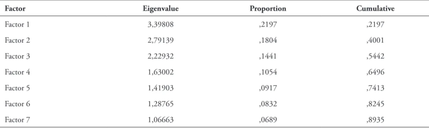
We extracted 7 factors from 28 variables using the principal factors method. These 7 factors account for 89 percent of the variance of the original variables (Table 1). This means there is not much loss of information when we substitute
ser vistos como “termos de erro”:
Representam a porção de
que não pode ser
explicada por
. A letra maiúscula grega gama (
) é uma matriz p
k da carga fatorial.
Como sugere o modelo, a análise fatorial assume que é possível representar um
conjunto de p
variáveis usando um número menor de fatores intrínsecos k. Contudo,
para que a análise fatorial seja bem-sucedida, deve haver correlações razoavelmente
fortes entre as variáveis usadas na análise. Em outras palavras, a matriz de correlação
dessas variáveis deve ser diferente da matriz identidade. Para verificar essa premissa,
usamos o teste de esfericidade de Bartlett, que rejeitou as hipóteses nulas de
esfericidade (p = ,000). Concluímos que a análise fatorial é adequada ao nosso conjunto
de dados.
Há diversos procedimentos de extração de fatores que podem ser utilizados. O
método de máxima verossimilhança (ML) tem a vantagem de permitir o teste da
materialidade estatística da carga fatorial. Esse método, no entanto, exige a premissa da
normalidade multivariada (FABRIGAR et al., 1999). Por meio do teste Doornik-Hansen
(DOORNIK; HANSEN, 2008), descobrimos que as variáveis usadas neste artigo
rejeitaram a hipótese nula da normalidade multivariada (p = ,000). Para evitar resultados
distorcidos, optamos pelo uso do método de fatores principais (PF) para a extração de
fatores. Esse método não tem premissas distribucionais.
3.3 ESTIMATIVA DO MODELO
Nos modelos probit e logit, a variável dependente
costuma ser expressa como
uma função de variável latente e observável I
ie um limiar desconhecido
(GUJARATI, 1995; POWERS; XIE, 2000):
(2)
Quando há erro de classificação na variável dependente, as condições acima não
são respeitadas. A variável observada y
inão é a mesma que a variável verdadeira
. O
modelo agora tem dois novos parâmetros α0
e α1
:
(3)
Em estudos sobre a FDF, o erro mais importante é o demonstrado como parâmetro
α1
na segunda equação. Esse erro é a probabilidade de a empresa que tenha emitido
demonstrações financeiras falsas não ser classificada com tal (erro tipo II). A
expectativa é de que o outro erro (tipo I) seja bastante raro e próximo a zero. Portanto,
para facilitar a convergência do modelo, este artigo adota a premissa de que α0
= 0. Sem
essa restrição, o valor esperado de y
iem um modelo logit é (HAUSMAN;
ABREVAYA; SCOTT-MORTON, 1998):
(4)
A função de log-verossimilhança foi efetivamente maximizada neste artigo, com
base na
equação 4, mas com a restrição α0
= 0, é:
(5)
ser vistos como “termos de erro”:
Representam a porção de
que não pode ser
explicada por
. A letra maiúscula grega gama () é uma matriz p k da carga fatorial.
Como sugere o modelo, a análise fatorial assume que é possível representar um
conjunto de p
variáveis usando um número menor de fatores intrínsecos k. Contudo,
para que a análise fatorial seja bem-sucedida, deve haver correlações razoavelmente
fortes entre as variáveis usadas na análise. Em outras palavras, a matriz de correlação
dessas variáveis deve ser diferente da matriz identidade. Para verificar essa premissa,
usamos o teste de esfericidade de Bartlett, que rejeitou as hipóteses nulas de
esfericidade (p = ,000). Concluímos que a análise fatorial é adequada ao nosso conjunto
de dados.
Há diversos procedimentos de extração de fatores que podem ser utilizados. O
método de máxima verossimilhança (ML) tem a vantagem de permitir o teste da
materialidade estatística da carga fatorial. Esse método, no entanto, exige a premissa da
normalidade multivariada (FABRIGAR et al., 1999). Por meio do teste Doornik-Hansen
(DOORNIK; HANSEN, 2008), descobrimos que as variáveis usadas neste artigo
rejeitaram a hipótese nula da normalidade multivariada (p = ,000). Para evitar resultados
distorcidos, optamos pelo uso do método de fatores principais (PF) para a extração de
fatores. Esse método não tem premissas distribucionais.
3.3 ESTIMATIVA DO MODELO
Nos modelos probit e logit, a variável dependente
costuma ser expressa como
uma função de variável latente e observável I
ie um limiar desconhecido
(GUJARATI, 1995; POWERS; XIE, 2000):
(2)
Quando há erro de classificação na variável dependente, as condições acima não
são respeitadas. A variável observada y
inão é a mesma que a variável verdadeira
. O
modelo agora tem dois novos parâmetros α
0e α
1:
(3)
Em estudos sobre a FDF, o erro mais importante é o demonstrado como parâmetro
α
1na segunda equação. Esse erro é a probabilidade de a empresa que tenha emitido
demonstrações financeiras falsas não ser classificada com tal (erro tipo II). A
expectativa é de que o outro erro (tipo I) seja bastante raro e próximo a zero. Portanto,
para facilitar a convergência do modelo, este artigo adota a premissa de que α
0= 0. Sem
essa restrição, o valor esperado de y
iem um modelo logit é (HAUSMAN;
ABREVAYA; SCOTT-MORTON, 1998):
(4)
A função de log-verossimilhança foi efetivamente maximizada neste artigo, com
base na
equação 4, mas com a restrição α
0= 0, é:
(5)
ser vistos como “termos de erro”: Representam a porção de que não pode ser explicada por . A letra maiúscula grega gama ( ) é uma matriz p k da carga fatorial.
Como sugere o modelo, a análise fatorial assume que é possível representar um conjunto de pvariáveis usando um número menor de fatores intrínsecos k. Contudo, para que a análise fatorial seja bem-sucedida, deve haver correlações razoavelmente fortes entre as variáveis usadas na análise. Em outras palavras, a matriz de correlação dessas variáveis deve ser diferente da matriz identidade. Para verificar essa premissa, usamos o teste de esfericidade de Bartlett, que rejeitou as hipóteses nulas de esfericidade (p = ,000). Concluímos que a análise fatorial é adequada ao nosso conjunto de dados.
Há diversos procedimentos de extração de fatores que podem ser utilizados. O método de máxima verossimilhança (ML) tem a vantagem de permitir o teste da materialidade estatística da carga fatorial. Esse método, no entanto, exige a premissa da normalidade multivariada (FABRIGAR et al., 1999). Por meio do teste Doornik-Hansen (DOORNIK; HANSEN, 2008), descobrimos que as variáveis usadas neste artigo rejeitaram a hipótese nula da normalidade multivariada (p = ,000). Para evitar resultados distorcidos, optamos pelo uso do método de fatores principais (PF) para a extração de fatores. Esse método não tem premissas distribucionais.
3.3 ESTIMATIVA DO MODELO
Nos modelos probit e logit, a variável dependente costuma ser expressa como uma função de variável latente e observável Ii e um limiar desconhecido
(GUJARATI, 1995; POWERS; XIE, 2000):
(2)
Quando há erro de classificação na variável dependente, as condições acima não são respeitadas. A variável observada yi não é a mesma que a variável verdadeira . O
modelo agora tem dois novos parâmetros α0e α1:
(3)
Em estudos sobre a FDF, o erro mais importante é o demonstrado como parâmetro
α1na segunda equação. Esse erro é a probabilidade de a empresa que tenha emitido
demonstrações financeiras falsas não ser classificada com tal (erro tipo II). A expectativa é de que o outro erro (tipo I) seja bastante raro e próximo a zero. Portanto,
para facilitar a convergência do modelo, este artigo adota a premissa de que α0 = 0. Sem
essa restrição, o valor esperado de yi em um modelo logit é (HAUSMAN;
ABREVAYA; SCOTT-MORTON, 1998):
(4)
A função de log-verossimilhança foi efetivamente maximizada neste artigo, com base na equação 4, mas com a restrição α0 = 0, é:
(5)
A função 5 foi maximizada por meio do método Newton-Raphson.
4 RESULTADOS
Extraímos 7 fatores das 28 variáveis usando o método de fatores principais. Esses 7 fatores são responsáveis por 89% da variação das variáveis originais (Tabela 1).Isso significa que não há grande perda de informações quando substituímos as 28 variáveis originais por esses 7 fatores no modelo logit.
A Tabela 2 mostra a carga fatorial de cada variável usada na análise fatorial (a
matriz Γ na Eq. 1). Cada variável é igual à soma dos produtos dos fatores pela carga
fatorial correspondente, mais seu escore único. Ao analisar os fatores absolutos mais altos de cada variável, podemos entender a composição de cada fator.
TABELA 1 – VARIAÇÃO EXPLICADA PELA ANÁLISE FATORIAL (MÉTODO DE FATORES PRINCIPAIS)
Fonte: Compilada pelos autores.
Fator Autovalor Proporção Cumulativo (todos os pontos na tabela devem ser substituídos por vírgula)
O primeiro fator (capaz de capturar quase 22 da variação das variáveis originais) parece estar relacionado positivamente com a saúde financeira das empresas. Relaciona-se positivamente com as variáveis EBITTA, ROA, zscore, WCTA, ΔWCTA. Além disso, relaciona-se negativamente com as variáveis TLTA e ΔTLTA. As empresas com menos dívida e ROA alto costumam apresentar valores do Fator 1 mais altos.
O Fator 2 captura 18% da variação das variáveis utilizadas. Relaciona-se positivamente com COGSAL, CASHTA e INVSAL, e negativamente com as variáveis ΔCOGSAL e EBITSAL. Esses resultados mistos sugerem que as empresas com mais recursos investidos em alguns tipos de ativo circulante (caixa e estoque) e com custos de vendas decrescentes (mas ainda altos) tendem a apresentar valores mais altos para o Fator 2. Esse fator relaciona-se negativamente com a avaliação da lucratividade (EBITSAL).
O Fator 3 relaciona-se positivamente com a CATA e negativamente com a
FATA. As empresas com mais ativos circulantes tendem a apresentar valores mais altos para o Fator 3. A variável ΔTLTE, embora bem capturada pelo Fator 3, conta com carga fatorial muito baixa para ser considerada significativa.
Factor Eigenvalue Proportion Cumulative
these 7 factors for the 28 original variables in the logit model.
Table 2 shows the factor loadings for each variable used in factor analysis (the matrix Γ in Eq. 1). Each variable is equal to the sum of the
products of the factors by their respective factor loadings, plus its unique score. Analyzing the highest absolute factors for each variable, we can understand the composition of each factor.
TABLE 1 – Variance explained by factor analysis (principal factors method)
Factor Eigenvalue Proportion Cumulative
Factor 1 3,39808 ,2197 ,2197
Factor 2 2,79139 ,1804 ,4001
Factor 3 2,22932 ,1441 ,5442
Factor 4 1,63002 ,1054 ,6496
Factor 5 1,41903 ,0917 ,7413
Factor 6 1,28765 ,0832 ,8245
Factor 7 1,06663 ,0689 ,8935
Source: The authors
The first factor (that is able to capture almost 22 percent of the variance in the original variables) seems to be positively related to the financial health of the companies. It is positively related to the variables EBITTA, ROA, zscore,
WCTA, ΔWCTA. It is also negatively related to the variables TLTA and ΔTLTA. Companies with less debt and high ROA usually present higher Factor 1 values.
Factor 2 captures 18 percent of the variance of the variables used. It is positively related to COGSAL, CASHTA and INVSAL, and is negatively related to variables ΔCOGSAL and EBITSAL. These mixed results suggest that companies with more resources invested in some kinds of current assets (cash and inventory) and decreasing (but still high) costs of sales tend to have higher values for Factor 2. This factor is also negatively related to a profitability measure (EBITSAL).
Factor 3 is positively related to CATA and negatively related to FATA. Companies with more current assets tend to present a higher Factor 3. The variable ΔTLTE, although mostly captured by Factor 3, has a factor loading too small to be meaningful.
Factor 4 is positively related to ΔCASHTA, ΔCATAand IETL. It is also negatively related to ΔFATA. This factor captures increases in cash and current assets. This factor captures well the increases and decreases of the variables included in Factor 3. Companies with high Factor 4 are changing the composition of their assets and also incurring in more interest expenses.
Factor 5 is positively related to ΔINVSAL and negatively related to ΔEBITTA and ΔROA. It is a variable that captures decreases in profitability and increases in inventory. This factor captures increases and decreases in some of the variables included in Factor 1.
There are no variables that have their highest absolute factor loading in Factor 7. The highest factor loadings associated with Factor 7 are the ones of ΔTLTA(0.406), WCTA (0.368) andΔROA(0.377). It seems that companies that increased their liabilities (but still have enough current assets to cover their current liabilities) and also improved their profitability tend to have a higher Factor 7. Companies with high Factor 7 are becoming more profitable possibly due to financial leverage.
476
Rev. bus. manag., São Paulo, Vol. 16, No. 52, pp. 466-483, Jul./Sept. 2014 Artur Filipe Ewald Wuerges / José Alonso Borba
variables that were not included in factor analysis. The least significant variable (the one with higher p-value) was eliminated, and the model was estimated again. This elimination procedure was repeated until all the remaining variables had p-values lower than 10 percent. The resulting model is shown in Table 3. It should be noted that the sample in each intermediary
model (and also in the final model) contained only the observations with data available for all the variables used in the initial model. Adding observations after dropping a variable, although possible, could generate biased estimates. Due to the large number of missing observations, the sample contained just 41 of the 118 cases of fraud originally identified.
TABLE 2 – Factor loadings and unique variances
Variable Factor 1 Factor 2 Factor 3 Factor 4 Factor 5 Factor 6 Factor 7 Uniqueness
COGSALt-1 -0,434 0,673 -0,504 -0,121 0,156 0,019 0,024 0,065 ΔCOGSALt-1 0,273 -0,460 0,420 0,139 -0,164 -0,088 -0,075 0,479 EBITSALt-1 0,439 -0,676 0,482 0,114 -0,154 0,011 0,015 0,080
EBITTAt-1 0,572 -0,249 -0,127 -0,182 0,271 0,023 0,283 0,408
ΔEBITTAt-1 -0,218 0,172 0,006 0,223 -0,466 0,235 0,261 0,533
ROAt-1 0,726 0,188 -0,261 -0,187 0,329 0,018 0,021 0,226
ΔROAt-1 -0,447 0,132 0,191 0,255 -0,468 0,180 0,377 0,287
zscoret-1 0,299 0,145 -0,080 0,003 -0,179 -0,203 -0,002 0,810
CACLt-1 0,181 0,324 0,129 0,047 -0,093 -0,356 -0,104 0,698
ΔCACLt-1 -0,050 -0,087 -0,018 -0,034 0,022 0,159 0,041 0,961 CASHTAt-1 0,175 0,556 0,299 0,186 -0,077 -0,479 -0,284 0,220
ΔCASHTAt-1 0,197 0,269 0,175 0,541 0,345 -0,017 0,211 0,403
WCTAt-1 0,660 0,310 -0,169 -0,156 -0,328 -0,153 0,368 0,148
ΔWCTAt-1 0,516 0,197 -0,281 0,404 -0,182 0,429 -0,275 0,160
TLTAt-1 -0,680 -0,210 0,317 0,149 0,303 0,184 -0,297 0,157
ΔTLTAt-1 -0,561 -0,156 0,349 -0,290 0,147 -0,413 0,406 0,099
TLTEt-1 0,001 -0,003 0,003 -0,009 0,003 0,012 0,004 1,000
ΔTLTEt-1 -0,003 -0,008 -0,009 0,007 0,000 -0,005 0,000 1,000
ARTAt-1 0,095 0,141 0,385 -0,379 0,069 0,461 0,058 0,459
INVSALt-1 -0,109 0,248 -0,163 -0,132 0,137 0,076 0,053 0,855 ΔINVSALt-1 -0,014 0,120 -0,137 -0,070 0,142 0,039 0,062 0,936
INVTAt-1 0,117 0,144 0,251 -0,293 0,055 0,328 0,151 0,683
CATAt-1 0,252 0,618 0,635 -0,255 0,020 0,093 -0,110 0,066
ΔCATAt-1 0,153 0,216 0,232 0,505 0,423 0,026 0,281 0,363
FATAt-1 -0,178 -0,478 -0,488 0,250 0,009 -0,120 0,113 0,413
ΔFATAt-1 -0,105 -0,181 -0,135 -0,364 -0,281 -0,059 -0,173 0,694
SALARt-1 -0,005 -0,018 -0,022 0,031 0,010 -0,014 0,019 0,998
IETLt-1 -0,065 -0,030 -0,058 0,098 0,036 0,026 0,043 0,978
Note. The factor with the highest absolute factor loading in each line is bolded.
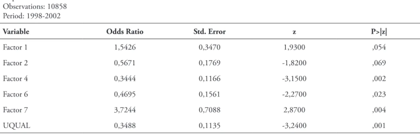
In the final model, five factors and one dummy variable (UQUAL) were significant at the 10 percent level. The model as a whole was also significant, with the likelihood ratio test
rejecting the null hypothesis at the 1 percent level (p = .0024); this means that the final model fits the data better than a model with only the intercept.
TABLE 3 – Logit model without misclassification parameter
Dependent variable: AAER Observations: 10858
Period: 1998-2002
Variable Odds Ratio Std. Error z P>|z|
Factor 1 1,5426 0,3470 1,9300 ,054
Factor 2 0,5671 0,1769 -1,8200 ,069
Factor 4 0,3444 0,1166 -3,1500 ,002
Factor 6 0,4695 0,1561 -2,2700 ,023
Factor 7 3,7244 0,7088 2,8700 ,004
UQUAL 0,3488 0,1135 -3,2400 ,001
LR χ2: 20,39
Prob > χ2: ,0024
Log-likelihood: -259,47
Source: The authors
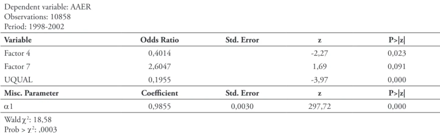
Taking into account the possibility of misclassification, we used the model from Table 3 as the initial model and performed a stepwise procedure. This procedure dropped three factors (1, 2 and 6), and the resulting model is shown in Table 4. Both remaining factors (4 and 7), while still rejecting the null hypothesis of the z-test, presented higher p-values in the model with a misclassification parameter. On the other hand, the variable UQUAL presented a lower p-value. The signs of the ratios of these variables remained unchanged. Since the Wald test rejected the null hypothesis, we conclude that at least one of the ratios of the variables used is statistically different from zero. The Wald test is asymptotically equivalent to the LR test used in the model without the misclassification parameter (ENGLE, 1984).
Companies with low Factor 4 and high Factor 7 are more likely to resort to fraud. Ceteris paribus, each increase by 1 in Factor 7 makes a company 2.6 times more likely to be involved in FSF. Since Factor 4 and UQUAL present odds ratios lower than 1, we decided to raise their odds ratios to the -1 power to better elucidate their influence on the likelihood of fraud. This way, each decrease by 1 in Factor 4 makes a company 2.49 times () more likely to be involved in fraud. Likewise, a company that did not receive an unqualified audit report is 5.12 times () more likely to be involved in fraud.