ISSN 2307-7743 http://scienceasia.asia
_______________
2010 Mathematics Subject Classification: 92B05.
Key words and phrases: Tuberculosis; Modeling; Reinfection; Bifurcation; Stability analysis.
© 2014 Science Asia 1 / 23 THE ROLE OF RE-INFECTION IN MODELING THE DYNAMICS OF ONE-STRAIN
TUBERCULOSIS INVOLVING VACCINATION AND TREATMENT GOODLUCK MIKA MLAY, LIVINGSTONE S. LUBOOBI, DMITRY KUZNETSOV, FRANCIS SHAHADA Abstract. In this article a continuous time deterministic model with vaccination and treatment strategies is formulated to assess the effect of reinfection on the transmission dynamics of Tuberculosis (TB). The involvement of reinfection in our model causes relapse and leads to the possibility of backward bifurcation at critical value of effective reproduction number Re 1and hence the existence of multiple equilibria when effective reproduction number Re 1. This indicates that even by reducing effective reproduction number
e
R below one is no longer a sufficient condition to eradicate the disease from community. An additional reduction of effective reproduction number Re below the saddle-node bifurcation value is required to eradicate disease from community provided that the disease free equilibrium is globally asymptotically stable. Numerical simulation results are presented to validate analytical results. We suggest that reinfection is an important feature of TB and has to be considered when modeling the complex dynamics of TB.
1. INTRODUCTION
Tuberculosis (TB) is a chronic bacterial infectious disease caused by pathogen Mycobacterium tuberculosis with more than one-third of the world human population as its reservoir [1, 9, 16]. A global annual estimate of 8.6 million people develop Tuberculosis, of which 1.3 million die from disease. It is reported in [24] that, the burden of disease caused by TB is high in developing world where poor nutrition, congested accommodation and emergency of HIV are manifested. The global estimates of incidence, prevalence and mortality rates per 100,000 population in 2012 were respectively 255, 303 and 26 and Tanzania incidence, prevalence and mortality rates per 100,000 population were 165, 176 and 13 respectively as per [24]. It therefore raises a quest to find desirable means to curtail TB morbidity and mortality rates.
sweats. Further symptoms are coughing, coughing up of sputum and/ or blood, shortness of breath and chest pains if the infection in the lung get worse [7]. TB draws back economics of the world and Tanzania in particular as it affects men than women and especially the productive working group [23]. In absence of HIV a small proportion of
about 10% of infected individuals with Mycobacterium tuberculosis develop TB and
2. MODEL FORMULATION
Our population model is subdivided into six compartments and is developed from the basic SEIT (Susceptible-Exposed-Infectious-Treated) compartmental model. A compartment of Vaccinated population (V ) is added to form SVEIT model. In addition compartment of
infectious population (I ) is subdivided into two compartments which are severely infected
population (I1) and mildly infected population (I2). Severely infected population (I1)
progresses faster to treatment group compared to mild infected population (I2). In this
model susceptible population will be recruited at a rate λ. Some susceptible individuals will come into contact with infectious individuals and being infected at a rate of β. A proportion, ρ of babies will be vaccinated at birth while the remaining proportion
1 ρ
will be left out of vaccination to join the susceptible population. Once vaccinated babies
loose immunity they become susceptible at per-capita rate θ , whereby 1/θ is the period
after which a vaccinated baby looses immunity. The Latently infected individuals progress to active TB through endogenous reactivation. The proportion (1η) of Latently infected individuals progresses fast to severely infected class, I1 while the remaining proportion, η
progresses slowly to mildly infected class, I2 at the same per-capita rate ε. Under usual circumstances mildly infected individuals take a long time to progress to treatment group,
T than severely infected individuals. That is a proportion, of mildly infected individuals
progresses to treatment group, T while the remaining proportion,
1
progresses to severely infected class, I1at the same per-capita rate ω. The severely infected individualsprogress to treatment group at a rate of υ. The treatment group, T is assumed to undergo
exogenous re-infection and relapse back to Latent group with infection level, γ. The infectious individuals I1 and I2 are assumed to die at disease induced mortality rates of δ1 and δ2 respectively while the rest die naturally at a rate of μ. All variables and parameters are assumed to be non-negative.
In addition the following assumptions are taken into consideration during the formulation of the model:
i. All individuals are born susceptible.
ii. The members of population mix homogeneously.
iii. Age, sex, social status, do not affect the probability of being infected.
iv. Natural recovery is negligible and hence ignored.
v. Vaccinated population looses immunity and become Susceptible.
vi. No more Vaccination can be administered to an individual infected with TB
vii. Once recovered from Treatment an individual reverts to be Latent and may experience another episode of disease.
viii. Once an individual is infected he/she will not recover if no treatment is given.
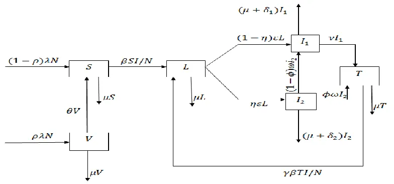
The above description of model formulation together with the assumptions leads to compartmental diagram in Figure 1.The full description of variables and parameters used to formulate the model are in Table 1 and Table 2 respectively:
Table 1: Description of variables of the model. Variable Description
) (t
S The Susceptible who are at risk of being infected at time t.
) (t
L The latently infected individuals at time t.
) (t
V Vaccinated individuals at time t.
) (
1 t
I Individuals who are severely infected with TB at time t.
) (
2 t
I Individuals who are mildly infected with TB at time t.
) (t
T Individuals Treated against TB at time t.
Table 2: Description of Parameters of the model. Parameter Description
Per capita birth rate.
β Per capita infection rate.
ρ Proportional of babies who are being vaccinated at birth.
θ The rate at which a vaccinated individual looses immunity.
ε The rate of progression from Latent class to both severely and mildly Infected
classes.
η Proportional of Latently infected population progressing to mild infected class.
μ Per capita natural death rate.
1
Per capita additional death rate of severely infected class.
2
Per capita additional death rate of mildly infected class.
Proportional of mildly infected class who are treated.
The rate at which a mildly infected individual is transferred to both severely
infected and treatment classes.
υ The rate at which a severely infected candidate is transferred to treatment
class.
γ The factor that reduces the level of reinfection.
2.1 Equations of the Model.
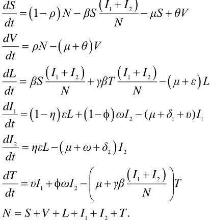
Basing on assumptions made and relationship that exists between variables and parameters shown in Figure 1 the system of six ordinary differential equations that describes the dynamics of tuberculosis in presence of vaccination and treatment is given by:
1 2
1 2 1 2
1
2 1 1
2
2 2 1 2
1 2
1 2
1
1 1 ( )
. I I dS
ρ N βS μS θV
dt N
dV
ρN μ θ V
dt
I I I I
dL
βS γβT μ ε L
dt N N
dI
η εL ωI μ δ υ I
dt dI
ηεL μ ω δ I
dt
I I dT
υI ωI μ γβ T
dt N
N S V L I I T
(1)
1 1 2 2dN
λ μ N δ I δ I
dt (2)
2.2 Normalization of the model.
The model (1) can easily be analyzed after being normalized such that the total population is one. The normalization is done by scaling the population of each compartment by total population. We transform the actual proportions by setting:
1 2
1 2
, , , I , I ,
S V L T
s v l i i h
N N N N N N
(3)
where by s v l i 1 i2 h 1.
Substituting (3) into (2) we end up with:
1 1 2 2
dN
λ μ δ i δ i N
dt (4)
Upon differentiating the proportions in (3) with respect to time t and make simplification,
leads to the following dimensionless system:
1 2 1 1 2 2
1 1 2 2
1 2 1 2 1 1 2 2
1
2 1 1 1 2 2 1
2
2 1 1 2 2 2
1 2 1 2 1 1 2 2
1 ,
,
,
1 1
. ,
, ds
ρ λ θv λ β i i δ i δ i s dt
dv
ρλ λ θ δ i δ i v dt
dl
βs i i γβh i i λ ε δ i δ i l dt
di
η εl ωi λ δ υ δ i δ i i
dt di
ηεl λ ω δ δ i δ i i dt
dh
υi ωi λ γβ i i δ i δ i h dt
(5)
subject to condition s v l i 1 i2 h 1. It can be shown that all the feasible solutions of system (5) enter the region of biological interest defined by
6
1 2 1 2
, , , , , : 1
s v l i i h s v l i i h
Ω
3. ANALYSIS OF A MODEL
We analyze model (5) in order to get some insights on dynamics of TB disease and transmission.
3.1 Existence and Local Stability of DFE
Let E0
s v l i i, , , 1, 2,h
be a DFE point of model (5). We set zero to the right hand side ofeach equation in (5) and assume that in absence of disease attack, l i1 i2 h 0 to solve the steady state solution. The disease free equilibrium point is therefore given by :
0 1 2
1
, , , , , θ λ ρ , ρλ , 0, 0, 0, 0
E s v l i i h
λ θ λ θ
. Before we prove for local stability of
DFE we define and determine the effective reproduction number, Re of model (5).
Definition 1. The effective reproduction number, Re is defined as the measure of average number of infections caused by a single infectious individual introduced in a community in which intervention strategies (in our case is treatment and vaccination) are administered [18].
The effective reproduction number Reis computed by using next generation operator
method [22] and found to be:
2
2 1 2
2 1
2 1
1 1 1
1 1 1
e
β θ λ ρ η λ ω δ ε ωηε ηε
R
λ θ λ ε λ ω δ λ δ υ λ ε λ ω δ
β θ λ ρ η λ ω δ ε ω λ δ υ ηε
λ θ λ ε λ ω δ λ δ υ
(6)
Theorem 3.1. The disease free equilibrium of model (5), given the effective reproduction
number, Re is locally asymptotically stable if Re 1 and unstable if Re 1.
We prove Theorem 3.1 for local stability of DFE by asserting that the trace and determinant of Jacobian matrix at DFE denoted by J E
0 are strictly negative and positive respectively.
1 1 2 2 0 1 2 0 00 0 0
0 0 0
0 0 1 1 0
0 0 0 0
1 0 0 1 0 1 1
θ λ ρ θ λ ρ
λ θ λ θ
ρλ ρλ
λ θ δ δ
λ θ λ θ
θ λ ρ θ λ ρ
λ ε
λ
λ θ β δ β δ
J E
β β
θ
η ε λ δ υ ω
ηε λ ω δ
υ ω θ λ λ
Trace and determinant of matrix J E
0 denoted by Tr
J E
0
and det
J E
0
arerespectively given by:
0
1 2
Tr J E 6λ θ ε υ ω δ δ 0 and
2 1 2 2 1 0 1 2 2 1 2 2 1 det 1 1 1 1 11 1 1
1 1
0
θ λ ρ θ λ ρ
λ ε
λ θ λ θ
λ θ
β θ λ ρ
η λ ω δ ε ω λ δ υ ηε
λ θ λ θ
λ ε λ ω δ λ δ υ
β θ λ ρ η λ ω δ ε ω λ δ υ ηε
β β
J E λ η ε λ δ υ ω
ηε
λ θ λ ε λ ω δ λ δ υ
λ ω δ
λ A
1 1 . e A R where 2
1 2 0
Aλ λ θ λ ε λ δ υ λ ω δ .
We find that Tr
J E
0
is strictly negative and det
J E
0
is strictly positive if and only if1 e
R . We therefore conclude that DFE is locally asymptotically stable.
3.2 Global Analysis of DFE of a model with interventions
0,
12
. .
n
n E n i
i
i
dX
A X X A X
dt dX A X dt (7)
From (7), Xn and Xi are vectors of non-transmitting and transmitting compartments
respectively.
0,
E n
X is a vector at disease free equilibrium point E0 of the same length as Xn. From model (5) we define:
1 2
0,
1 ,
, , , , , , , 0 ?
T
T T
n i E n
X s v h X θ λ ρ ρλ
λ θ λ
l i
θ
i X
and
0,
1
n E n
θ λ ρ
λ θ ρλ λ θ s
X X v
h
. For global stability of DFE we need to show that matrix A
has real negative eigenvalues and A2 is a Metzler matrix (i.e. the off-diagonal elements of
2
A are non-negative, symbolically denoted by A x2
ij 0, i j). Using system (5), then the first and second equations in (7) can be written respectively in expanded form as:
1 2 1 1 2 2 1 1 2 2
1 2 1 2 1 1 2 2
1 1 2 1
1
θ λ ρ
λ θ
ρ λ θv λ β i i δ i δ i s
ρλ
ρλ λ θ δ i δ i v A
λ θ
υi ωi λ γβ i i δ i δ i h
s
l
v A i
i h and
1 2 1 2 1 1 2 2
2 1 1 1 2 2 1 2 1
2 1 1 2 2 2 2
1 1
βs i i γβh i i λ ε δ i δ i l l
η εl ωi λ δ υ δ i δ i i A i
ηεl λ ω δ δ i δ i i i
. For compatibility, matrices A A, 1
and A2 should be of order 3 3 . By using non-transmitting elements from Jacobian matrix
of system (5) and representation in (7) we find that:
1 2 1 1 1 2 2 0 00 0 , 0
0 0 0
λ θ β δ s β δ s
A λ θ A δ δ
λ υ
v v
γβ γβ
h δ ω h δ
1 2 1 1 2 22 2 1
1 2
1 1 1
1
λ ε δ l δ l
η ε λ δ i δ i
ηε δ i λ ω δ i
β s γh β s γh
A υ ω
. We find that A is upper triangular
matrix whose eigeinvalues are located on its main diagonal. Therefore eigenvalues of A (i.e.
, and
λ λ θ λ
) are real and negative. In addition A2 is a Metzler matrix since its
off-diagonal elements are non-negative. That is 0l i i h, , ,1 2 1 and both
1i1
and
1i2
arestrictly positive. Therefore DFE for system (5) is globally asymptotically stable in region Ω. We have established important theorem:
Theorem 3.2. The disease-free equilibrium point is globally asymptotically stable in Ω if
1 e
R and unstable if Re 1.
3.3 Existence of Endemic Equilibrium Point (EEP) of model with interventions
Let 2
* * 1* *
2
, , , , ,
E s v l i i h be an endemic equilibrium point of model (5). The conditions of
existence of endemic equilibrium point E2 are obtained by setting the right hand side of each equation in (5) equal to zero and solve model (5) in terms of force of infection
* * *
1 2
f β i i at steady state. Let kλδ i1 1*δ i2 2*0, for any pairwise choice of i1
and i2 values at endemic equilibrium. An endemic equilibrium point in terms of force of infection is given by:
2 22 1 1 2
2 1
2 1 1 2
1 2
1
1 1 1
1 1 1
1
λ θ k ρ
s
f k θ k
ρλ v
θ k
λ ω δ k η ω δ k ωη θ k ρ γf k f
l
η f k θ k ε k ω δ k γf k δ υ k εγf υa a
λε η ω δ k ωη θ k ρ γf k f
i
f k θ k ε k ω δ k γf k δ υ k εγf υa a
ληε θ k ρ γf k δ υ k f
i
2 1 1 2
1 2
2 1 1 2
1 2 2 1
1
we define, 1 1 ;
f k θ k ε k ω δ k γf k δ υ k εγf υa a
λε θ k ρ υa a f
h
f k θ k ε k ω δ k γf k δ υ k εγf υa a
a η ω δ k ωη a ωη δ υ k
If we substitute representations of * 1
i and *
2
i from (8) into the force of infection,
* * *
1 2
f β i i or *
* *
1 2 0
f β i i we find that:
2 1
2 1 1 2
1 1 1
0
λε θ k ρ γf k f η ω δ k ωη η δ υ k
f β
f k θ k ε k ω δ k γf k δ υ k εγf υa a
(9)
Manipulating and simplifying (9) we end up with the following cubic polynomial:
2
1 1 1
0
f
A f
B f
C
(10)where by
1
1 1 1
1 1 1
,
, .
A γ M υP Q θ k
B k M γ M υP Q θ k βa γ P δ υ k ηε
C k Mk βa P δ υ k ηε
(11)
Furthermore in terms of parameters of model (5) we define:
2
1
M θ k ε k ω δ k δ υ k ; P
1 η ω δ
2 k ε
1
ωηε;
1
Q ωηε δ υ k and a1λ θ k
1ρ
. We write C1 in the following format:
1
1
2
2 1 e
θ k ε k ω δ k δ υ k k R
C
(12)
From (12),
22 1 0
θ k ε k ω δ k δ υ k k and Re is effective reproduction
number as indicated in (6).
From (10), f β i
1 i2
0
corresponds to Disease Free Equilibrium (DFE) that we have
already discussed while 2
1 1 1 0
A f B fC , that can be also be written in the form:
2
1 1 1 1
*
1
4 2
B B A C
f
A
(13)
Satisfies Endemic Equilibrium. The value of A1 is strictly positive. Depending on the signs
of B1 and C1 we have three cases to consider in order to have positive root of force of infection as follows:
Case 1: In absence of re-infection we find that the parameter for level of reinfection, γ0.
This implies from (11) that A10. The polynomial 2
1 1 1 0
A f B fC becomes linear, i.e.
1 1 0
B fC or * 1
1
C f
B
. If B10 then system (5) has stable endemic equilibrium when
1 0
C . This equilibrium happens when Re 1as interpreted from (12). In this case
Case 2: Exactly one endemic equilibrium point. From (13), suppose B10 and C10 or
2
1 4 1 1 0
B AC . This means the polynomial has just one positive root and hence the system
(5) has unique endemic equilibrium. Case 3: Two endemic equilibria If B10, C10 and 2
1 4 1 1 0
B AC , then the polynomial 2
1 1 1 0
A f B fC has two
positive roots. This means that the system (5) has two endemic equilibria and hence the possibility of backward bifurcation. These three cases are summarized under the following theorem:
Theorem 3.3: The number of positive endemic equilibria of Tuberculosis model (5) is
hereunder summarized as follows:
i. If C10, Re 1, the system has a unique endemic equilibrium.
ii. If B10 and C10 or 2
1 4 1 1 0
B AC , the system has exactly one endemic
equilibrium.
iii. If B10, C10 and 2
1 4 1 1 0
B AC , the system has exactly two endemic equilibria.
iv. Otherwise there are no endemic equilibria, i.e. when AC1 10 and B10.
From (iii), the critical point of effective reproduction number c e
R at which a backward
bifurcation occurs is computed by setting the discriminant in (13) equals to zero. Thus,
2
1 4 1 1 0
B AC implies that
2 2
1 4 1 2 1 1 0
c e
R
B A θk ε k ω δ k δ υ k k and,
2 1
2
1 2 1
1 4
c e
B
A θ k ε k ω δ k δ υ k k
R
. Thus backward bifurcation occurs in the
range c 1
e e
R R . Furthermore, we note from (13) that disease will be endemic if force
of infection is strictly positive (i.e. f0) and both B1 and AC1 1 are strictly negative. Thus,
1 0
A and
2
1 1 1 2 1 1 e 0
AC A θ k ε k ω δ k δ υ k k R if and only if Re 1.
Therefore endemic equilibrium point 2
1
* * * *
2
, , , , ,
E s v l i i h is stable if and only if Re 1. 3.4 Stability of Endemic Equilibrium Point (EEP) of model with intervention
that 6 1 1 i i x
. We define vector X
x x x x x x1, 2, 3, 4, 5, 6
T and F
f f1, 2,f3, f4,f5,f6
T insuch a way that the model (5) is re-written in the form dX F
dt as follows:
1 1 2 4 5 1 4 2 5 1
2 2 1 4 2 5 2
3 3 1 4 5 6 4 5 1 4 2 5 3
4 4 3 5 1 1 4 2 5 4
5 5 3 2 1 4 2 5 5
6 6 4 5 4
1 ?
,
1 1 ,
,
,
x f ρ λ θx λ β x x δ x δ x x
x f ρλ λ θ δ x δ x x
x f βx x x γβx x x λ ε δ x δ x x
x f η εx ωx λ δ υ δ x δ x x
x f ηεx λ ω δ δ x δ x x
x f υx ωx λ γβ x
x5
δ x1 4 δ x x2 5
6. (14)
The Jacobian matrix J E
0 of system (14) at disease free equilibrium E0 presented in Section 3.1 is given by
1 1 2 1
1 2 2 2
1 1
1
2 0
0 0
0 0 0
0 0 0
0 0 0
0 0 0 0
0
1
0
1
0
λ θ β δ r β δ r
λ θ δ r δ r
λ ε βr βr
η ε λ δ υ ω
ηε λ ω δ
υ E ω λ J (15)
From (15) we define r1 θ λ
1 ρ
λ θ
and 2
ρλ r
λ θ
. In particular case when basic
reproduction number Re 1, we choose our bifurcation parameter be β and consider our
bifurcation to take place at ββ
. Solving β from (6) when Re 1 we find that:
1
1
2
2
1
1 1
λ θ λ ε λ ω δ λ δ υ
β β
θ λ ρ η λ ω δ ε ω λ δ υ ηε
(16)
The Jacobian of transformed system (14) at ββ
has simple zero eigenvalue that allows
us to study the dynamics of the system (5) at β β using Centre Manifold theory [4]. The
Jacobian of (14) denoted by J E
0 at β β has right eigenvector that corresponds withzero eigenvalue given by
1, 2, 3, 4, 5, 6
T
w w w w w w
1 1 1 2 1 1 1 2 2 2 1
1 5
1
1 2 2 1 2 2 1
2 5 1 2 3 5 2 1 4 5 1 5 5 6 0, 0, 0, 0, free
,
.
k β r ηε δ r θ β δ λ θ r β r ηε δ r θ β δ λ θ r
w w
λ λ θ β r ηε
δ r λ ε λ ω δ β r ηε δ r β r ηε
w w
λ θ β r ηε
λ ω δ
w w
ηε
λ ε λ ω δ β r ηε
w w
β r ηε
w w υ w
2
1 15 1
0.
λ ε λ ω δ β r ηε ωβ r ηε
w λβ r ηε
(17)
From (17), k1
λ ε λ ω δ
2
β r ηε1 and 1
1θ λ ρ
r
λ θ
. By using (16) we show that
1
k is strictly positive justifying that the components w w w2, 4, 6 0 as follows:
2 1 1 2 2 1 1 2 2 1 1 2 2 1 1 1 11 1 1
1 0.
1 1
λ ε λ ω δ β r ηε
β r ηε λ ε λ ω δ
λ ε λ ω δ
λ θ λ δ υ r ηε λ ε λ ω δ
θ λ ρ η λ ω δ ε ω λ δ υ ηε
λ δ υ ηε λ ε λ ω δ
η λ ω δ ε ω λ δ υ η
k ε
Moreover, the Jacobian matrix J E
0 at β β
has left eigenvector
1, 2, 3, 4, 5, 6
T
Ψ Ψ Ψ Ψ Ψ Ψ Ψ
associated with zero eigenvalue satisfying the relation Ψ 1, where by:
1
1
1 2 6 3 4 4 4 5 4
1 2
1
0, λ δ υ 0, 0, ω λ δ υ 0.
Ψ Ψ Ψ Ψ Ψ Ψ Ψ Ψ Ψ
β r λ ω δ
(18)
We compute the value of a and b that will govern totally the local dynamics of system (14)
Theorem 3.4. Consider the general system of ordinary differential equations (14) with a
parameter β such that dx
,
, : nf x β f
dt and
2 n
f , where 0 is an
equilibrium point of the system (i.e. f
0,β
0 for all β) and1.
0, 0 i
0, 0x
j
f A D f
f
is Jacobian (linearization) matrix of the system around
the equilibrium 0 with β evaluated at 0,
2. Zero is a simple eigenvalue of A and other eigenvalues of A have negative real
parts;
3. Matrix A has a right eigenvector and a left eigenvector Ψ corresponding to zero
eigenvalue.
Let fk be the th
k component of f and
2 , , 1
0, 0
n
k
k i j
k i j i j
f
a Ψ w w
x x
and
2 , 1
0, 0 n
k k i k i i
f
b Ψ w
x β
then the local dynamics of the system around the equilibriumpoint 0 is totally determined by the signs of a and b. In particular, if a0 and 0
b then a backward bifurcation occur at β0. Signs of a and b play the vital
role in describing the local dynamics of model (14) around equilibrium point 0 as
follows:
a) a0,b0, whenβ0 with β 1, 0 is locally asymptotically stable and there exists a positive unstable equilibrium, when 0 β 1 , 0 is unstable and there exists a negative and locally asymptotically stable equilibrium.
b) a0,b0 , when β0 with β 1 , 0 is unstable, when 0 β 1 , 0 is
asymptotically stable and there exists a positive unstable equilibrium.
c) a0,b0, when β0 with β 1, 0 is unstable and there exists a locally
asymptotically stable negative equilibrium, when 0 β 1, 0 is stable and a
positive unstable equilibrium appears.
d) a0,b0 when β changes from negative to positive, 0 changes its stability from stable to unstable. Correspondingly, negative unstable equilibrium becomes positive and locally asymptotically stable.
Computation of a and b
We compute the value of a and b that will govern totally the local dynamics of system (14)
a and b by employing Theorem 4.1 of Castillo-Chavez and Song [6] and as implied in Theorem 3.4 of this article.
Since the components of left eigenvector Ψ Ψ1 2 Ψ6=0 (for k1, 2 and 6) we compute the values of a and bfor only k 3, 4,5. The only non-zero second order partial derivatives of (14) at DFE when β β are:
2 2 2 2 2 2
* *
3 3 3 3 4 5
1 2
2 2
1 4 1 5 4 6 5 6 4 5
,
, , 2 2 .
f f f f f f
β γβ δ δ
x x x x x x x x x x
By using
2 , , 1
0, 0 n
k k i j k i j i j
f a Ψ w w
x x
we compute a as follows:
* * * *
3 1 4 1 5 3 4 1 3 5 2 4 6 5 6
2 2
4 4 1 4 5 2 5 4 5 1 5 2
* *
3 1 4 5 6 3 4 5 4 1 3 3 4 4 5 5
5 2 3 3 4 4 5 5
2
2
2
2
.
Ψ w w β w w β w w δ w w δ w w γβ w w γβ
Ψ w δ w w δ Ψ w w δ w δ
Ψ β w w w w γΨ β w w w δ Ψ w Ψ w Ψ w
a
w δ Ψ w Ψ w Ψ w
(19)
On the other hand, the value of b is computed by using the formula,
2 , 1
0, 0 n
k k i k i i
f
b Ψ w
x β
.The associated non-zero second order partial derivatives of (14) at DFE when β β
and
3, 4,5
k are:
2 2
3 3
1
4 5
1
θ λ ρ
f f
x
x β x β λ θ
The value of b is therefore given by:
3 4 5 3 4 5
1 1 1
0
θ λ ρ θ λ ρ θ λ ρ
Ψ w w Ψ w w
λ θ λ λ
b
θ θ
(20)
From (19), let 1 * 1
3 4 5
Ψ β w w
ζ w and
*
2 6 3 4 5 4 1 3 3 2 4 4 5 5 5 2 3 3 4 4 2 5 5
ζ w γΨ β w w w δ Ψ w Ψ w Ψ w w δ Ψ w Ψ w Ψ w . It follows that the sign of a depends on the value of w1. If w10 or w10 and ζ2ζ1 then a0. We
formulate the following theorem.
Theorem 3.5: If w10 or w10 and ζ2ζ1, a0 then model (5) exhibits backward bifurcation at Re 1. If β0 then there exists unstable positive endemic equilibrium point
and correspondingly if β 0 then there exists a stable negative endemic equilibrium point.
Figure 2: Bifurcation diagram showing backward bifurcation with estimated parameters
14
β ;γ1.8;θ0.8;ε 0.396 ;η 0.1 ;λ 0.9 ;δ10.3;ω0.6; ρ0.1; ν0.9;δ20.2
ω=0.6; and 0.1 for numerical simulation.
Figure 2 shows the backward bifurcation of system (5) that occurs at threshold parameter
1 e
R , due to presence of multiple equilibria and re-infection. DFE stands for Disease Free
equilibrium and EE stands for Endemic Equilibrium. In the neighborhood of 1 when Re 1
then stable DFE coexists with two endemic equilibria: the small unstable EE (with smaller number of TB infectives) and larger stable endemic equilibrium with large number of infectives. This implies that even with classically reducing the threshold parameter to less than unity does not clear TB from community. That is why we say backward bifurcation is
an undesirable feature of TB. When Re 1 then we have two equilibria: unstable DFE and
large stable EE. According to Buonomo and Lacitignola [3] if Re is nearly below one then
disease control depends on initial sub-populations of the model under consideration. That is reducing Re below the critical value c 1
e
R eradicate disease from community given that
the disease free equilibrium is globally asymptotically stable.
3.5 Global Stability of Endemic Equilibrium Point of a model with intervention.
In this section we prove the global stability of endemic equilibrium point E2 of system (5)
by using Lyapunov's direct method. Our Lyapunov function is constructed from suitable choice of logarithmic function. The global properties of endemic equilibrium point are studied by stating and proving the following theorem.
Theorem 3.6 If Re 1 then the unique endemic equilibrium E2 of system (5) is globally
Proof: We use approach of Korobeinikov [13] as it is used to most complicated compartmental epidemiological models, to construct the Lyapunov function from suitable choice of the following logarithmic function:
*
, ln
i i
i i
W
a y y ywhere ai are properly chosen positive constants, yi is population of compartment i and
i
y is the equilibrium level. We define the function
1 2 1 2
: , , , , , : , , , , , 0
W s v l i i h Ω s v l i i h by:
* * *
1 2 1 2 3
* * *
4 1 1 1 5 2 2 2 6
, , , , , ln ln ln
ln ln ln .
W s v l i i h A s s s A v v v A l l l
A i i i A i i i A h h h
The constants A A1, 2, A6 are non-negative in Ω and W is Lyapunov function. The
function W together with its constants A A1, 2, A6 0 are chosen in such way that W is
continuous and differentiable in a space 1
C and on the interior of Ω, E2 is global
minimum of W on Ω , and
* * * * * *
1 2
, , , , , 0
W s v l i i h . The time derivative of Lyapunov
function W computed along the solutions of system (5) is:
*
* * *
1 1
1 2 3 4
1
* *
2 2
5 6
2
1 1 1 1
1 1 .
i di
s ds v dv l dl
W A A A A
s dt v dt l dt i dt
i di h dh
A A
i dt h dt
(21)
At Endemic equilibrium point (EEP) we have:
* * * * * *
1 2 1 1 2 2
* * *
1 1 2 2
* * * * * * * * *
1 2 1 2 1 1 2 2
*
* * * *
1 * 2 1 1 2 2
1 *
* *
2 * 1 1 2 2
2
* * * * *
1 2 1 2 1 1 2
*
1 ,
1
,
1 1
,
,
1 ,
1
ρ λ λ β i i δ i δ i s θv
ρλ λ θ δ i δ i v
λ ε βs i i γβh i i δ i δ i l
l
λ δ υ η εl ωi δ i δ i
i ηεl
λ ω δ δ i δ i
i
λ υi ωi γβ i i δ i δ i
h
*
2.
(22)
*
* * * * * *
1 1 2 1 1 2 2 1 2 1 1 2 2
*
* * *
2 1 1 2 2 1 1 2 2
*
* * * * * * * * *
3 1 2 1 2 * 1 2 1 2 1 1 2 2 1 1 2
1
s s
W A λ β i i δ i δ i s θv θv λ β i i δ i δ i s
s
v v
A λ θ δ i δ i v λ θ δ i δ i v
v
l l
A βs i i γβh i i βs i i γβh i i δ i δ i l δ i δ
l l
* 2 *
* * * * * *
1 1
4 2 * 2 1 1 2 2 1 1 1 2 2 1 1
1 1
*
* * * * *
2 2
5 * 1 1 2 2 2 1 1 2 2 2 2
2 2
*
* *
6 1 2 * 1 2
1
1 1 1 1
1
1
i l l
i i
A η εl ωi η εl ωi δ i δ i i δ i δ i i i
i i
i i
A ηεl ηεl δ i δ i i δ i δ i i i
i i
h h
A υi ωi υi ωi γβ
h h
* * * * * * *
1 2 1 1 2 2 1 2 1 1 2 2
i i δ i δ i h γβ i i h δ i δ i h h
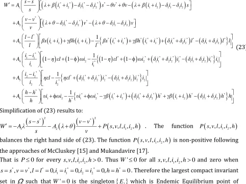
(23)
Simplification of (23) results to:
*
2
*
2
1 2 , , , , ,1 2
s s v v
W A λ A λ θ P s v l i i h
s v
. The function P s v l i i h
, , , , ,1 2
balances the right hand side of (23). The function P s v l i i h
, , , , ,1 2
is non-positive followingthe approaches of McCluskey [15] and Mukandavire [17].
That is P0 for every s v l i i h, , , , ,1 2 0. Thus W'0 for all s v l i i h, , , , ,1 2 0 and zero when
* * * * * *
1 1 2 2
0 0 0
, , , , , 0
ss vv l l i i i i hh . Therefore the largest compact invariant
set in Ω such that W'0 is the singleton
E2 which is Endemic Equilibrium point of model (5). LaSalles's invariant principle [14] then implies that E2 is globally asymptotically stable in the interior of the region Ω if Re 1and that completes our proof.4. NUMERICAL SIMULATIONS AND DISCUSSIONS
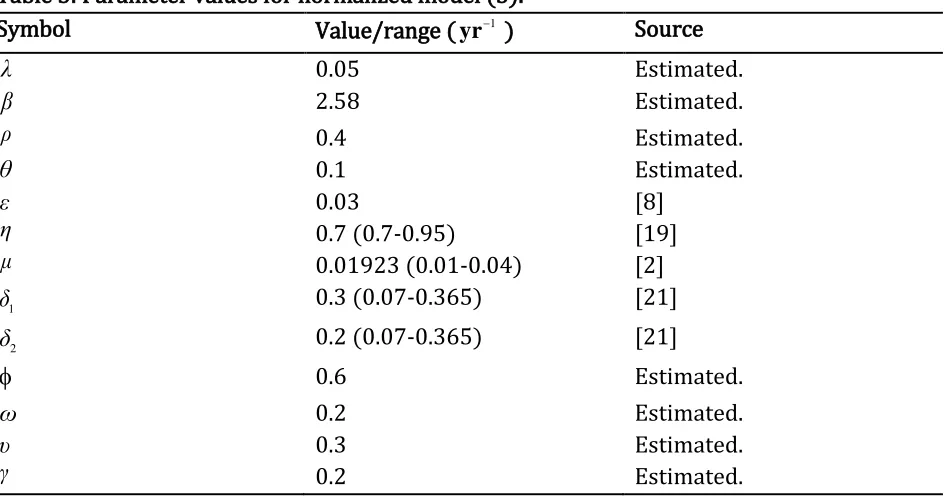
Table 3: Parameter values for normalized model (5).
Symbol Value/range ( 1
yr ) Source
λ 0.05 Estimated.
β 2.58 Estimated.
ρ 0.4 Estimated.
θ 0.1 Estimated.
ε 0.03 [8]
η 0.7 (0.7-0.95) [19]
μ 0.01923 (0.01-0.04) [2]
1
δ 0.3 (0.07-0.365) [21]
2
δ 0.2 (0.07-0.365) [21]
0.6 Estimated.
ω 0.2 Estimated.
υ 0.3 Estimated.
γ 0.2 Estimated.
4.1 Numerical Simulation of a model (5) in presence of intervention and TB.
Figure 3: Shows the dynamics of susceptible, vaccinated, latently infected, severely infected, mildly infected and treated population proportions in presence of interventions and TB with increasing time.
Figure 3 shows dynamic behavior of susceptible, vaccinated, latently infected, severely infected, mildly infected and treated classes when Re 1.8519. The plot is produced by MATLAB by using β2.58;γ0.2;θ0.1;ε0.03;η0.7;λ0.05;δ10.3;ω0.2;
2 0.4; 0.3; 0.2
ρ ν δ 0.6 as estimated parametric values and whose definitions are
given in Table 2. Starting with initial values s
0 0.60,v
0 0.05,l
0 0.1,i1
0 0.1,0 50 100 150 200 250
0 0.1 0.2 0.3 0.4 0.5 0.6 0.7
time in years
Po
pu
la
tio
n
Pr
op
or
tio
ns
Susceptible Vaccinated Latently infected Severely infected mildly infected treated
s(0)=0.6, v(0)=0.05, l(0)=0.1, i1(0)=0.1, i
2(0)=0.1, h(0)=0.05.
2 0 0.1i and h
0 0.05, the system (5) attains the local asymptotic stability of endemicequilibrium point,
*
2
* * * * * 1 2
, , , , , 0.4170, 0.1383, 0.3497, 0.0069, 0.0165, 0.0716
E s v l i i h . In
presence of interventions and TB, susceptible population proportion initially decreases to lower levels and later increases to its carrying capacity with time as shown in Figure 3. Vaccinated population proportion initially increases to higher levels and stabilizes as time increases. On the other hand both latently infected and treated population proportions increase to higher levels and gradually decreases to their carrying capacities. However both mildly and severely infected population proportions decreases to their lowest endemic levels. Again even with intervention, disease does not clear from community since effective reproduction number is Re 1.8519 1 . Classically this result supports the theorem of local stability of endemic equilibrium.
4.2 Phase portraits illustrating dynamical behavior of population proportions at EEP.
In this section phase portraits to illustrate the dynamics of the model (5) at endemic equilibrium point for susceptible class versus vaccinated, latently infected, severely infected, mildly infected, and treated classes are plotted by using parameter values indicated in Table 3. With different varying initial conditions, each solution curve in Figure
4 tends to endemic equilibrium point E2 presented in Section 4.1. Therefore we conclude
that the system (5) is globally stable about endemic equilibrium point E2 for the
parameters displayed in Table 3.
5. CONCLUSION
In this article, a continuous time deterministic Tuberculosis model with vaccination and treatment as intervention strategies has been formulated and the role of reinfection on transmission dynamics of TB is critically assessed. In presence of reinfection and multiple
equilibria the backward bifurcation occurs at effective reproduction number Re 1. In this
scenario stable disease free equilibrium coexists with two endemic equilibria: smaller unstable endemic equilibrium (with small number of infected individuals) and larger stable endemic equilibrium (with large number of infected individuals) in the neghbourhood of 1 when Re 1. This shows that even with classically reducing the threshold Re below one the disease still persist in the community. We suggest that reinfection is a real TB feature and an important aspect to consider when modeling the complex dynamics of TB.
REFERENCES
[1] B. R. Bloom, Tuberculosis: Pathogenesis, Protection and Control, Washington, D.C., ASM Press (1994). [2] S. M. Blower, A. R. Mclean, T. C. Porco, P. M. Amall, M. A. Sanchez, and R. Moss, The intrinsic transmission dynamics of tuberculosis epidemics, Nature Medicine, 1 (1995), 815-821.
[3] B. Buonomo, and D. Lacitignola, On the backward bifurcation of a vaccination model with nonlinear incidence, Nonlinear Analysis: Modelling and Control, 16(1) (2011), 30–46.
[4] J. Carr, Applications of Center Manifold Theory, Springer-Verlag, New York, (1981).
[5] C. Castillo-Chavez, Z. Feng, and W. Huang, Mathematical Approaches for Emerging and Re-emerging Infectious Diseases, An Introduction. Springer Verlag, (2002).
[6] C. Castillo-Chavez, and B. Song, Dynamical models of tuberculosis and their applications, Mathematical Biosciences and Engineering, 1 (2004), 361-404.
[7] T. Cohen, M. Murray, On modeling epidemics of multidrug-resistant M. tuberculosis of heterogeneous fitness, Nature Medicine 10 (2004), 1117-1121.
[8] T. Cohen, C. Colijn, B. Finklea, and M. Megan, Exogenous Re-infection and the Dynamics of Tuberculosis Epidemics: Local Effects in a Network Model of Transmission, J. R. Soc. Interface 4 (2007), 523-531.
[9] Z. Feng, C. Castillo-Chavez, and A. F. Capurro, A model for tuberculosis with exogenous reinfection, Theor. Popul. Biol. 57 (2000), 235–247.
[10] A. B. Gumel, and S. M. Moghadas, A qualitative study of a vaccination model with non-linear incidence, App. Math. Comput. 143 (2003), 409–419.
[11] H. W. Hethcote, The mathematics of infectious diseases, SIAM Review 42 (2000), 599-653.
[12] S. Kim, S. Choe, J. Kim, S. Nam, Y. Shin, and S. Lee, What Does a Mathematical Model Tell About the Impact of Reinfection in Korean Tuberculosis infection?, Osong Public Health Res Perspect. 5(1) (2014), 40-45. [13] A. Korobeinikov, Lyapunov functions and global properties for SEIR and SEIS epidemic models, Mathematical Medicine and Biology. 21(2004): 75–83.
[14] J. P. LaSalle, The stability of dynamical systems. CBMS-NSF in Regional Conference Series in Applied Mathematics. No. 25. SIAM, Philadelphia. (1976).
[15] C. C. McCluskey, Lyapunov functions for tuberculosis models with fast and slow progression, Mathematical Biosciences and Engineering, 3(4) (2006), 603–614.