Vol 8, No 6 (2017)

Available online throug

ISSN 2229 – 5046

International Journal of Mathematical Archive- 8(6), June – 2017 197

APPROXIMATE ANALYTICAL SOLUTION OF

NON LINEAR EQUATION IN BIOLOGICAL MEMBRANE USING SINGLE PARAMETER HPM

M. SYED IBRAHIM

a

_{, T. ISWARYA}

b

_{, R. ASHOKAN}

a

_{, L. RAJENDRAN}

c,*

a

_{Department of Mathematics,}

School of Mathematics, Madurai Kamaraj University, Madurai, Tamilnadu, India.

b

_{Department of Mathematics,}

Alagappa Govt. Arts and science college, Karaikudi, Tamilnadu, India.

c

_{Department of Mathematics,}

SethuInstitute of Technology, Pullor, Kariyapatti, Tamilnadu, India.

Received On: 12-05-17; Revised & Accepted On: 03-06-17)

ABSTRACT

T

raditional perturbation methods depend on a small parameter which is difficult to be found for real-life nonlinear problems. To overcome this problem, in this article a powerful analytical methods (single parameter homotopy perturbation method (HPM)) is applied to solve nonlinear differential equation in biological membrane. Proper graphs will be used to illustrate the obtained results. The proposed analysis demonstrates reliability and efficiency applicability of the employed method. In this paper we obtained the approximate analytical solutions for the non linear equations under non steady state conditions using single parameter homotopy perturbation method. Simple and approximate polynomial expressions for the concentration of spices are obtained.

Keywords: Mathematical Modeling; nonlinear equations; single parameter homotopy perturbation method.

1. INTRODUCTION

The transport of molecules across biological membranes is vital to the operation and survival of living cells. The supply of nutrients to the cell, for growth and reproduction, and the transfer of waste products from cell to the extracellular medium, is a complex process that is facilitated by many mechanisms. There is passive transport of molecules due to the combined effects of concentration gradients and electrical potential differences that exist across the cell membrane. Neutral molecules diffuse from regions of high concentration to regions of low concentration. In addition, charged molecules move along a voltage gradient that normally exists across a cell membrane, such as in neural cells and axons. Carrier-mediated transport and active transport are additional mechanisms that facilitate the movement of molecules across cell boundaries. The transport mechanism of molecules may be model using nonlinear ordinary and partial differential equations.

There are many nonlinear equations, which are quite useful and applicable in engineering and physics such as the well-known KdV equation [1], MKdV equation, BBM equation [2], Burgers equation [2], KdV–KSV equation [2], so on. Since solving these equations needs some nonphysical assumptions, some various approximate methods have recently been developed to solve linear and nonlinear differential equations [3–9]. Recently many non linear problems are solved using homotopy perturbation method (HPM) [10–12] and variational iteration method (VIM) [13–15], which are widely applied to various engineering problems [16–30]. In this article the non linear problem in biological membrane is presented and the single parameter homotopy perturbation method are employed to compute an approximation to the solution of the system of nonlinear differential equations governing the problem.

Corresponding Author: L. Rajendran

c,*,

© 2017, IJMA. All Rights Reserved 198

2. MATHEMATICAL FORMULATION OF THE PROBLEM

The system of equations in biological membrane can be represented as follows:

2 1

y

dt

dy

₌

(1) 3 2

y

dt

dy

₌

(2) 4 3

y

dt

dy

=

(3)

5 4 3 2 1

4

₃

_y

₆

_y

₂

_y

₅

_y

_y

dt

dy

+

−

+

+

−

=

(4)

5

5

_y

dt

dy

₌

₋

(5)

The initial conditions are:

1

)

0

(

,

2

)

0

(

,

5

.

1

)

0

(

,

1

)

0

(

,

5

.

0

)

0

(

2 3 4 5

1

=

y

=

y

=

y

=

y

=

y

(6)

where

y

_i are the concentration of the species in thin membrane.

This problem is nonlinear, however, the following similar transformations may be applied:

1

y

z

=

(7)

2 1

_y

dt

dy

dt

dz

=

=

(8)

3 2 2 2

y

dt

dy

dt

z

d

₌

₌

(9)

dt

dy

dt

z

d

₃ 3 3

=

(10)

Make the substitutions into the above set of Eqns. (7) – (10) to obtain the below Eqns.

2 1

y

dt

dy

₌

(11) 3 2

y

dt

dy

₌

(12) 3 2 1 3 2 1 3

2

y

y

y

y

dt

dy

−

+

=

(13)

Single-parameter hpm solution

The single-parameter HPM solution is quite attractive as it gives a compact analytical solution which can serve several purposes. It can give a deeper insight into the physics of the problem. It can give a rough first-hand idea about the mathematical structure of the solution (for example, presence of boundary layers etc.). It can be launching pad for obtaining a more accurate solution using a numerical iterative technique. Further, if it gives sufficiently accurate results then there is no need to look any further for other solutions. The homotopy perturbation equations corresponding to Eqns. (11) and (13)are written as

(

1

)

0

2 2 1

2

1

+

+

−

−

=

y

b

y

p

y

b

dt

dy

(14)

(

2

)

0

2 3 2

2

2

+

+

−

−

=

y

b

y

p

y

b

dt

dy

(15)

(

2

_{1 2}3 ₁2 ₃ 2 ₃

)

0

3 2

3

+

_b

_y

+

_p

−

_y

−

_y

+

_y

_y

−

_b

_y

=

dt

dy

(16)

where p is the homotopy perturbation parameter and b is an auxiliary parameter whose value will be calculated by

© 2017, IJMA. All Rights Reserved 199

(

_{2 1}

)

0

1

1

+

_y

+

_p

−

_y

−

_y

=

dt

dy

(17)

(

3 2

)

0

2

2

+

+

−

−

=

y

y

p

y

dt

dy

(18)

(

2

3 3

)

0

2 1 3 2 1 3

3

+

+

−

−

+

−

=

y

y

y

y

y

p

y

dt

dy

(19)

The initial conditions are:

1

)

0

(

,

2

)

0

(

,

3

)

0

(

2 3

1

=

y

=

y

=

y

(20)

Seeking the perturbation solutions for the concentration of species

y

₁

,

y

₂and

y

₃ as under

....

12 2 11 10

1

y

p

y

p

y

y

=

+

+

(21)

....

22 2 21 20

2

y

p

y

p

y

y

=

+

+

(22)

....

32 2 31 30

3

y

p

y

p

y

y

=

+

+

(23)

Substitute the Eqns. (21) – (23) in Eqns. (17) – (19) we obtain the following systems of equations for zeroth and first order. Zeroth-order system:

0

0

0

30 30 20 20 10

10

+

=

+

=

+

=

y

dt

dy

y

dt

dy

y

dt

dy

(24)

The initial conditions are

1

)

0

(

,

2

)

0

(

,

3

)

0

(

20 30

10

=

y

=

y

=

y

(25)

First-order system:

0

2

0

0

30 30 2 10 3 20 10 31 31 20 30 21 21 20 10 11 11

=

−

+

−

−

+

=

−

−

+

=

−

−

+

y

y

y

y

y

y

dt

dy

y

y

y

dt

dy

y

y

y

dt

dy

(26)

The initial conditions are

0

)

0

(

,

0

)

0

(

,

0

)

0

(

20 30

10

=

y

=

y

=

y

(27)

The solution of the zeroth-order system is straightforward. We have

( )

( )

( )

t

in t

in t

in

e

y

t

y

e

y

t

y

e

y

t

y

₁₀

(

)

=

₁ − ₂₀

(

)

=

₂ − ₃₀

(

)

=

₃ −

(28)

Substituting for

y

₁₀

,

y

₂₀and

y

₃₀in Eq. (26) and solving the differential equations for

y

₁₁

,

y

₂₁and

y

₃₁ applying the appropriate initial conditions, we get

( )

( )

t

in t

in

t

e

y

t

e

y

t

y

₁₁

(

)

=

₁ −

+

₂ − (29)

( )

( )

t

in t

in

t

e

y

t

e

y

t

y

₂₁

(

)

=

₃ −

+

₂ − (30)

( ) ( )

_{( )}

( )

_{( )}

t

( )

in

( ) ( )

in in t

in t in t in t in in

e

y

y

y

e

t

y

e

y

e

t

y

e

y

y

t

y

− −

− − −

















−

+

+

−

+

=

2

2

2

2

2

)

(

3 2 1 3 2 3 3 3 2 1 3 3 2 1

31 ₍₃₁₎

© 2017, IJMA. All Rights Reserved 200

( )

( )

( )

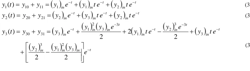
t

in t

in t

in

e

y

t

e

y

t

e

y

y

y

t

y

1

(

)

=

10

+

11

=

1 −

+

1 −

+

2 − (32)

( )

( )

( )

t

in t

in t

in

e

y

t

e

y

t

e

y

y

y

t

y

₂

(

)

=

₂₀

+

₂₁

=

₂ −

+

₃ −

+

₂ − (33)

( )

( ) ( )

( )

( )

( )

( ) ( ) ( )

in in in t

t in t in t in t in in t in

e

y

y

y

e

t

y

e

y

e

t

y

e

y

y

e

y

y

y

t

y

− − − − − −

















−

+

+

−

+

+

=

+

=

2

2

2

2

2

)

(

3 2 1 3 2 3 3 3 2 1 3 3 2 1 3 31 30 3 (34)

RESULT AND DISCUSSION

Equations (32)- (34) represent the new analytical expression of concentrations of species in biological membrane. Fig

1 represent the concentration

y

₁ versus time t for various values of initial concentration. From Fig 1a-1b, it is observed

that, the concentration

y

₁ increases with the initial values of the concentration. Also the concentration

y

₁ decreases

when time increases when initial value is greater than two (refer Fig 1a). But the concentration

y

₁ initially rises and reaches the maximum value immediately and then decreases gradually.

Fig 2, represent concentration

y

₂ versus time t. From these figure, it is inferred that when the initial values increases,

the concentration is also increases. Fig 3, represent the concentration of

y

₃ versus time t. Here also the concentration

decreases when initial values are increases. Fig 4, represent that the concentration of

y

₁

,

y

₂and

y

₃ versus time t for some initial values.

CONCLUSION

The approximate analytical expression of concentration of species in biological membrane is obtained by solving the nonlinear rate equation using single parameter homotopy perturbation method. First time we attempted the single parameter HPM solution for biological membrane which generally leads to a very good approximate solution in the minimum number of iteration.. Based on the proposed model, nonlinear equation in physical and chemical sciences is solved. These analytical results are useful for experimental data analysis.

APPENDIX A: Basic Concept of Homotopy Perturbation Method

To explain this method, let us consider the following function:

r

,

0

)

(

)

(

u

−

f

r

=

∈

Ω

D

_o

(A1) with the boundary conditions of

r

,

0

)

,

(

=

∈

Γ

∂

∂

n

u

u

B

_o (A2)

where

D

_o is a general differential operator,

B

_o is a boundary operator,

f

(

r

)

is a known analytical function and

Γ

is the boundary of the domain

Ω

. In general, the operator

D

_o can be divided into a linear part

L

and a non-linear part

N

. The eqn. (A.1) can therefore be written as

0

)

(

)

(

)

(

u

+

N

u

−

f

r

=

L

(A3)

By the homotopy technique, we construct a homotopy

v

(

r

,

p

)

:

Ω

×

[

0

,

1

]

→

ℜ

that satisfies

.

0

)]

(

)

(

[

)]

(

)

(

)[

1

(

)

,

(

v

p

=

−

p

L

v

−

L

u

0

+

p

D

v

−

f

r

=

H

o (A4)

.

0

)]

(

)

(

[

)

(

)

(

)

(

)

,

(

v

p

=

L

v

−

L

u

₀

+

pL

u

₀

+

p

N

v

−

f

r

=

H

(A5)

Where p

∈

[0, 1] is an embedding parameter, and

u

₀ is an initial approximation of eqn. (A1) that satisfies the boundary conditions. From eqns. (A4) and (A5), we have

0

)

(

)

(

)

0

,

(

v

=

L

v

−

L

u

₀

=

H

(A6)

0

)

(

)

(

)

1

,

(

v

=

D

v

−

f

r

=

© 2017, IJMA. All Rights Reserved 201 When p=0, the eqns. (A4) and (A5) become linear equations. When p =1, they become non-linear equations. The process of changing p from zero to unity is that of

L

(

v

)

−

L

(

u

₀

)

=

0

to

D

_o

(

v

)

−

f

(

r

)

=

0

. We first use the embedding parameter

p

as a “small parameter” and assume that the solutions of eqns. (A.4) and (A.5) can be written as a power series in

p

:

...

2 2 1

0

+

+

+

=

v

v

p

v

p

v

(A8)

Setting

p

=

1

results in the approximate solution of the eqn. (A1):

...

lim

_{0 1 2} 1

+

+

+

=

=

→

v

v

v

v

u

p

(A9)

This is the basic idea of the HPM.

Figure-1: Concentration

y

₁ versus time t for various value of initial concentration.

© 2017, IJMA. All Rights Reserved 202

Figure-3: Concentration

y

₃ versus time t for various value of initial concentration.

Figure-4: Concentrations

y

₁

,

y

₂

,

y

₃versus time t.

REFERENCES

Study on nonlinear Jeffery Hamel flow by He's semi-analytical methods and comparison with numerical results Z.Z. Ganji, D.D. Ganji, M. Esmaeilpour

1. D. Kaya, An explicit and numerical solutions of some fifth-order KdV equation by decomposition method, Applied Mathematics and Computation 144 (2003) 353–363.

2. K. Al-Khaled, Approximate wave solutions for generalized Benjamin–Bona–Mahony–Burgers equations, Applied Mathematics and Computation 171 (2005) 281–292.

3. D.D. Ganji, The application of He’s homotopy perturbation method to nonlinear equations arising in heat transfer, Physics Letters A (in press).

4. D.D. Ganji, Solitary wave solutions for a generalized Hirota–Satsuma coupled KdV equation by homotopy perturbation method, Physics Letters A (in press).

5. D.D. Ganji, Assessment of homotopy–perturbation and perturbation methods in heat radiation equations, International Communications in Heat and Mass Transfer 33 (3) (2006) 391–400.

6. C. Jin, M. Liu, A new modification of Adomian decomposition method for solving a kind of evolution equation, 169 (2005) 953–962.

7. G. Adomian, A review of the decomposition method in applied mathematics, Journal of Mathematical Analysis and Applications 135 (1988) 501–544.

8. J.H. He, Some asymptotic methods for strongly nonlinear equations, International Journal of Modern Physics B 20 (2006) 1141–1199.

9. J.H. He, Non-Perturbative Methods for Strongly Nonlinear Problems, Dissertation.de-Verlag im Internet GmbH, Berlin, 2006.

© 2017, IJMA. All Rights Reserved 203 11. J.H. He, A coupling method of a homotopy technique and a perturbation technique for non-linear problems,

International Journal of Non- Linear Mechanics 35 (1) (2000) 37–43.

12. J.H. He, New interpretation of homotopy perturbation method, International Journal of Modern Physics B 20 (2006) 2561–2568.

13. J.H. He, Variational iteration method—a kind of nonlinear analytical technique: Some examples, International Journal of Non-linear Mechanics 34 (4) (1999) 699–708.

14. J.H. He, Approximate analytical solution for seepage with fractional derivatives in porous media, Computational Methods in Applied Mechanics and Engineering 167 (1998) 57–68.

15. J.H. He, Approximate solution of nonlinear differential equations with convolution product nonlinearities, Computational Methods in Applied Mechanics and Engineering 167 (1998) 69–73.

16. J.H. He, Homotopy perturbation method: A new nonlinear analytical technique, Applied Mathematics and Computation 135 (1) (2003) 73–79.

17. J.H. He, The homotopy perturbation method for nonlinear oscillators with discontinuities, Applied Mathematics and Computation 151 (1) (2004) 287–292.

18. J.H. He, Periodic solutions and bifurcations of delay-differential equations, Physics Letters A 347 (4–6) (2005) 228–230. D.D. Ganji et al. / Computers and Mathematics with Applications 54 (2007) 1018–1027 19. J.H. He, Application of homotopy perturbation method to nonlinear wave equations, Chaos, Solitons and

Fractals 26 (3) (2005) 695–700.

20. Rajendran, Kirthiga, Laborda, Mathematical modeling of nonlinear reaction–diffusion processes in enzymatic biofuel cells, Current Opinion in Electrochemistry (2017), 21. J. Saranya, L. Rajendran, L. Wang, C. Fernandez, A new mathematical modelling using Homotopyperturbation

method to solve nonlinear equations in enzymatic glucose fuel cells, Chemical Physics Letters 662 (2016) 317–326.

22. S. Pavithra, L. Rajendran, R.Ashokan, Analytical Solution Of The Nonlinear Initial Value Problem In One-Stage Thermophilic Bioremediation Process For The Treatment Of Cheese Whey, Asian Journal of Current Engineering and Maths 5:4 July - August (2016) 44 – 51.

23. Malinidevi Ramanathan, Rasi Muthuramalingam, Rajendran Lakshmanan, The Mathematical Theory of Diffusion and Reaction in Enzymes Immoblized Artificial Membrane. The Theory of the Non-Steady State, J Membrane Biol., July 2015.

24. R. Malini Devi, O. M. Kirthiga, L. Rajendran, Analytical Expression for the Concentration of Substrate and Product in Immobilized Enzyme System in Biofuel/Biosensor, Applied Mathematics, 2015, 6, 1148-1160. 25. M. Rasi,a L. Rajendran, and M. V. Sangaranarayanan Enzyme-Catalyzed Oxygen Reduction Reaction in

Biofuel Cells: Analytical Expressions for Chronoamperometric Current Densities, Journal of The Electrochemical Society, 162 (9) H671-H680 (2015).

26. K. Saravanakumar, L. Rajendran, M.V. Sangaranarayanan, Current–potential response and concentration profiles of redox polymer-mediated enzyme catalysis in biofuel cells – Estimation of Michaelis–Menten constants, Chemical Physics Letters 621 (2015) 117–123.

27. P.Sivakuma, R.Muthuramalingam. R, Rajendran. L, Analytical expressions for the concentrations of dimethyl sulphide (DMS) in gas and liquid phase, Molecular Enzymology and Drug Targets, Vol. 1 No. 1:5 (2015). 28. D. Mary Celin Sharmila, T. Praveen, and L. Rajendran, Mathematical Modeling and Analysis of Nonlinear

Enzyme Catalyzed Reaction Processes, Journal of Theoretical Chemistry, Volume 2013, Article ID 931091, 7 pages,

29. V. Ananthaswamy, SP. Ganesan, L. Rajendran, Approximate analytical solution of non-linear boundary value problem in steady state flow of a liquid film: Homotopy perturbation method, Int. Journal of Applied Sciences and Engineering Research, Vol. 2, No. 5, 2013.

30. Mehala N, Ananthaswamy V, Rajendran L, Analytical Solutions of Fluroscent Reporters to auxin influx in plantcells, International Journal of Innovative Research in Science, Engineering and Technology, 3(3), 2014, 2347 – 6710.

Source of support: Nil, Conflict of interest: None Declared.