Vol 4, No 11 (2013)

Available online through

A NEW TYPE OF TRANSPORTATION PROBLEM USING OBJECT ORIENTED MODEL

R. Palaniyappa

_{and V. Vinoba}

1_{Department of Mathematics, IRT Polytechnic College, Chromepet, Chennai – 44, India.}

2_{Department of Mathematics, K. N. G. C. (W), Thanjavur – 7, India.}

(Received on: 07-10-13; Revised & Accepted on: 30-10-13)

ABSTRACT

I

Keywords: Transportation problem, LPP, optimal solution, south east corner rule, object oriented programming.

1. INTRODUCTION

The term ‘OR’ was coined in 1940 by M. C. Closky & T.ref then in a small town of Bawdsey in England. It is a science that came into existence in a military content. During world war II, the military management of UK called an Scientists from various disciplines & organized them into teams to assist it in solving strategic & tactical problems relating to air & land defence of the country.

The transportation problem is a special class of LPP that deals with shipping a product from multiple origins to multiple destinations. The objective of the transportation problem is to find a feasible way of transporting the shipments to meet demand of each destination that minimizes the total transportation cost while satisfying the supply & demand constraints. The two basic steps of the transportation method are

Step 1: Determine the initial basic feasible solution

Step 2: Obtain the optimal solution using the solution obtained from step 1.

In this paper we introduce the new type of transportation problem called South east corner rule. I have presented that the proposed south east corner rule for finding optimal solution of a transportation problem do not reflect optimal solution continuously. Three examples are provided to my claim. Also by the North west corner rule process optimal solutions are showed to illustrate the comparison.

2. MATHEMATICAL STATEMENT OF THE TRANSPORTATION PROBLEM

A. In developing the LP model of the transportation problem the following notations are used ai - Amounts to be shipped from shipping origin i (ai≥ 0 .

bj - Amounts to be received at destination j (bj≥ 0).

cij - Shipping cost per unit from origin i to destination j (cij≥ 0).

xij - Amounts to be shipped from origin i to destination j to minimize the total cost (xij≥ 0).

We assumed that the total amount shipped is equal to the total amount received, that is,

∑ 𝑎𝑎𝑚𝑚𝑖𝑖=1 𝑖𝑖≥ ∑𝑛𝑛𝑗𝑗=1𝑏𝑏𝑗𝑗.

Corresponding author: R. Palaniyappa1*

B. Transportation problem

Min ∑𝑚𝑚_𝑖𝑖=1∑𝑛𝑛_𝑗𝑗=1𝑐𝑐_{𝑖𝑖𝑗𝑗}𝑥𝑥_{𝑖𝑖𝑗𝑗} .

Subject to ∑𝑛𝑛_𝑗𝑗=1𝑥𝑥_{𝑖𝑖𝑗𝑗}≤ai , i = 1 , 2 , … , m

∑ 𝑥𝑥𝑚𝑚𝑖𝑖=1 𝑖𝑖𝑗𝑗 = bj , j = 1 , 2 , … , n , where 𝑥𝑥𝑖𝑖𝑗𝑗≥ 0 ∀ i , j .

Feasible solution: A set of non negative values 𝑥𝑥_{𝑖𝑖𝑗𝑗} , i = 1 , 2 , …, n and j = 1 , 2 , …, m that satisfies the constraints is called a feasible solution to the transportation problem .

Optimal solution: A feasible solution is said to be optimal if it minimizes the total transportation cost.

Non degenerate basic feasible solution: A basic feasible solution to a (m × n) transportation problem that contains exactly m + n – 1 allocations in independent positions.

Degenerate basic feasible solution: A basic feasible solution that contains less that m + n – 1 non negative allocations.

Balanced and Unbalanced Transportation problem: A Transportation problem is said to be balanced if the total supply from all sources equals the total demand in the destinations and is called unbalanced otherwise.

Thus, for a balanced problem, ∑ 𝑎𝑎𝑚𝑚_{𝑖𝑖=1 𝑖𝑖} =∑𝑛𝑛_𝑗𝑗=1𝑏𝑏_𝑗𝑗 and for unbalanced problem, ∑ 𝑎𝑎𝑚𝑚_{𝑖𝑖=1 𝑖𝑖}≠∑𝑛𝑛_𝑗𝑗=1𝑏𝑏_𝑗𝑗 .

3. SOUTH EAST CORNER RULE

In this section, we introduce a new method called the south east corner rule for finding an optimal solution to a transportation problem. This method is similar to that of north west corner rule. The south east corner rule proceeds as follows.

This method starts at the south east corner cell (route) of the table variable (x43).

Step 1: Construct the transportation table for the given TPP.

Step 2: Allocate as much as possible to the selected cell and adjust the associated amounts of supply and demand by subtracting the allocated amount.

Step 3: Cross out the row or column with zero supply or demand to indicate that no further assignments can be made in that row or column. I both a row and column net to zero simultaneously, cross out one only and leave a zero supply (demand in the uncrossed out row - column).

Step 4: If exactly one row or column is left uncrossed out, stop. Otherwise, move to the cell to the right if a column has just been crossed out. Go to step 2 [8].

3.1 Numerical examples:

Problem 3.1: Obtain the IBFS of a Transportation problem whose cost & rim requirement table is given below

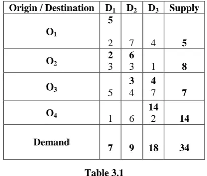
Solution: By applying south east corner rule process allocations are obtained as follows:

Since ∑𝑎𝑎_𝑖𝑖 = ∑ 𝑏𝑏_𝑗𝑗 there exists a feasible solution to the transportation problem.

We obtain initial feasible solution as follows:

Origin / Destination D1 D2 D3 Supply

O1 2 7 4 5

O2 3 3 1 8

O3 5 4 7 7

Table 3.1

The initial basic feasible solution is given by

x43 = 14, x33 = 4, x32 = 3, x22 = 6, x21 = 2, x11 = 5.

Total cost = 2 × 14 + 7 × 4 + 4 × 3 + 3 ×6 + 3 × 2 + 2 × 5 = 28 + 28 + 12 + 18 + 6 + 10

= 56 + 30 + 16 = Rs.102.

By applying North west corner rule the allocations are obtained as follows

The initial basic feasible solution is given by

x11 = 5, x21 = 2, x22 = 6, x32 = 3, x33 = 4, x43 = 14.

Total cost = 2 × 5 + 2 × 3 + 6 × 3 + 3 × 4 + 4 ×7 + 2 × 14 = Rs. 102.

Commits: The South east corner rule process shows that the optimal solution is Rs. 102 and it is exact and North west corner rule gives the same result.

Problem 3.2: Solve the transportation problem when the unit transportation costs, demands and supplies are as given below.

Solution: By applying south east corner rule process allocations are obtained as follows:

Origin / Destination D1 D2 D3 Supply

O1

5

2 7 4 5

O2

2

3

6

3 1 8

O3 ₅

3

4

4

7 7

O4

1 6

14

2 14

Demand

7 9 18 34

Origin / Destination D1 D2 D3 Supply

O1

5

2 7 4 5

O2

2

3

6

3 1 8

O3 ₅

3

4

4

7 7

O4

1 6

14

2 14 Demand

7 9 18 34

Origin / Destination D1 D2 D3 D4 Supply

O1 6 1 9 3 70

O2 11 5 2 8 55

O3 10 12 4 7 70

Since the total demand ∑𝑏𝑏_𝑗𝑗 = 215 is greater than the total supply∑𝑎𝑎_𝑖𝑖 = 195, the problem is an unbalanced TP.

We convert into a balanced TP by introducing a dummy origin O4 with cost zero and giving supply equal to

215 – 195 = 20 units. Hence, we have the converted problem as follows:

Table 3.2

Table 3.3

Total cost matrix:

The initial basic feasible solution is given by

x44 = 20, x34 = 25, x33 = 45, x23 = 5, x22 = 35, x21 = 15, x11 = 70.

Total cost = 0× 20 + 7 × 25 + 4 ×45 + 2×5 +5×35 +11×15 + 6 × 70 = Rs.1010.

By applying north west corner rule process allocations are obtained as follows:

Origin / Destination D1 D2 D3 D4 Supply

O1 6 1 9 3 70

O2 11 5 2 8 55

O3 10 12 4 7 70

O4 0 0 0 0 20

Demand 85 35 50 45 215

Origin / Destination D1 D2 D3 D4 Supply

O1 70

6 1 9 3 70

O2 15

11

35

5

5

2 8 55

O3

10 12

45

4

25

7 70

O4 _{0 0 0}

20

0 20

Demand 85 35 50 45 215

70

6 1 9 3

15

11

35

5

5

2 8

10 12

45

4

25

7

0 0 0

20

0

65

6

5

1 9 3

11

30

5

25

2 8

10 12

25

4

45

7

20

The initial basic feasible solution is given by

X11 = 65, x12 = 5, x22 = 30, x23 = 25, x33 = 25, x34 = 45, x41 = 20.

Total cost = 6 × 65 + 5 × 1 + 5 × 30 + 2 ×25 + 4 × 25 + 7 × 45 + 0 × 20 = Rs.1010.

Commits: The South east corner rule process shows that the optimal solution is Rs. 1010 and it is exact and North west corner rule gives the same result.

4. COMPARISON

In this section we compare the relationship between the transportation problem like south west corner rule and north west corner rule, least cost method. The numerical examples are given below.

Problem 4.1: Obtain initial basic feasible solution to the following transportation problem using south east corner rule and north west corner rule, least cost method, VAM.

Origin D E F G Available

A 11 13 17 14 250

B 16 18 14 10 300

C 21 24 13 10 400

Requirements 200 225 275 250

Solution: By applying North west corner rule the allocations are obtained as follows:

Origin D E F G Available

A 200

11

50

13 17 14 250

B 16 175 18

125

14 10 300

C 21 24 150 13

250

10 400

Requirements 200 225 275 250

The IBFS is

x11 = 200, x12 = 50, x22 = 175, x23 = 125, x33 = 150, x34 = 250.

Total cost = 11 × 200 + 13 × 50 + 18 × 175 + 14 × 125 + 13 × 150 + 10 × 250 = Rs. 12, 200

By applying Least cost method the allocations are obtained as follows:

Origin D E F G Available

A 200

11

50

13 17 14 250

B

16

50

18 14

250

10 300

C

21

125

24

215

13 10 400

Requirements 200 225 275 250

The IBFS is

x11 = 200, x12 = 50, x22 = 50, x24 = 250, x32 = 125, x33 = 215.

By applying Vogels Approximation method the allocations are obtained as follows:

200

11

50

13 17 14

16 175 18 14

125

10

21 24 275 13

125

10

The IBFS (using north west corner rule) is

x11 = 200, x12 = 50, x22 = 175, x24 = 125, x33 = 275, x34 = 215.

Total cost = 11 × 200 + 13 × 50 + 18 × 175 + 10 × 125 + 13 × 275 + 10 × 125 = 12,075

By applying South east corner rule the allocations are obtained as follows:

200

11

50

13 17 14

16

175

18

125

14

250

10

21

125

24

150

13

125

10 The IBFS is

x11 = 200, x12 = 50, x22 = 175, x23 = 125, x24 = 250, x32 = 125, x34 = 125, x33 = 150.

Total cost = 10 × 125 + 13 × 150 + 24×125 + 14×125 + 18 × 175 + 10 × 250 + 11 × 200 +13 ×50. = Rs.10, 625

Commits: The South east corner rule processes shows that the optimal solution is Rs.10, 625 whereas North west corner rule, least cost method and VAM gives the wrong results which are not optimal.

5. SOLVING TRANSPORTATION PROBLEM USING JAVA LANGUAGE

In this section we solve the transportation problem (south east corner and North West rule) using JAVA language. The main ideas from design Java programs are save time, money and effort.

5.1 JAVA Program me:

In Problem 3.1, we use the java programs to minimize the cost of transportation and determine the number of units transported from source i to destination j.

The results are shown as follows:

The result of south east corner program by JAVA language is the cost of transportation = Rs. 102.

The number of units transported from source i to destination j

We transport

Supply [3] to demand [2] = 14

Supply [2] to demand [2] = 4

Supply [2] to demand [1] = 3

Supply [1] to demand [1] = 6

Press any key to continue

The result of north west corner program by JAVA language is the cost of transportation = Rs. 102.

The number of units transported from source i to destination j

We transport

Supply [0] to demand [0] = 5

Supply [1] to demand [0] = 2

Supply [1] to demand [1] = 6

Supply [2] to demand [1] = 3

Supply [2] to demand [2] = 4

Supply [3] to demand [2] = 14

CONCLUSION

Running the above JAVA programs, the result of the programs are equal to LP solution but the solution using JAVA language faster and easier then LP solution. There is scope for further development of these topics.

REFERENCES

1. Abdallah.A, Hlayel, Mohammad. A.Alia, Solving Transportation problems using the best candidate method”, Computer science & Engineering: An international journal (CSEIJ), Vol.2, No.5, October 2012.

2. Dantzig, G.B, “Linear programming and extensions”, Princeton, NJ: Princeton University Press 1963.

3. Juman, Z.A. M. S. Hoque, M.A., Buhari, M.I. “study of transportation problem and use of object oriented programming”, 3rd conference on applied mathematics and pharmaceutical (ICAMPS ‘2013), April 29 - 30, 2013 singapore.

4. Mohammad KamrulHasan, “Direct methods for finding optimal solution of a transportation problem are not always reliable”, International journal of Engineering and Science (IRJES), Volume 1, Issue 2 (October 2012), pp 46 – 52.

5. Nabendusen et al, “A study of transportation problem for an essential item of southern part of north east region of India as an OR model and use of object oriented programming”, International journal of computer science and network security, 10 (4), pp 78 - 86, 2010.

6. Rao, S.S (1987) Optimization Theory and Applications. Wiley Eastern Limited.

7. Reeb, J.E. and S.A., Leavengood, “Transportation problem a special case for linear programming problems”, EM8779, Corvallis: Oregon state university extension service, pp 1- 35, 2002.

8. Sen, N. and Som, T. (2008a) Mathematical Modeling of Transportation Related Fare Minimization Problem of South-Assam and an Approach to Its Optimal Solution. IJTM, Vol. 32, nr. 3, pp. 201-208.

9. Sen, N. and Som, T. (2008c) Mathematical Modeling of Transportation Related Problem of Southern Assam with an Approach to Its Optimal Solution. ASR, Vol. 22, nr. 1, pp. 59-67.

10. Wilson, A.G; Coelho, J.D; Macgill, S.M and Williams, H.C.W.L (1981) Optimization in Locational and Transport Analysis. John Willey and Sons.

11. Hamdy A. Taha.” Operations Research: An Introduction, “Prentice Hall, 7 editions 5, USA, 2006.

12. Prem Kumar Gupta, D.S. Hira. “Operations Research”, An Introduction, S. Chand and Co., Ltd., New Delhi. 1999.