Genetic Algorithm Aided Antenna
Placement in 3D and Parameter
Determination Considering
Electromagnetic Field Pollution
Constraints
Tomislav Rolich and Darko Grundler
Faculty of Textile Technology, University of Zagreb, CroatiaThis paper presents genetic algorithm based method for antenna placement in 3D space and parameter deter-mination satisfying environmental electromagnetic field pollution constraints. The main goal is to find out antenna parameters(power, position in 3D, azimuth and elevation)in the area of interest so that electromagnetic field satisfies minimal electromagnetic field strength for service availability and, at the same time, be below prescribed limit in restricted subareas(people populated areas). The proposed method is validated with two real world antenna types and with seven different terrain configurations(various restricted areas). Besides finding the most optimal antenna parameters, the method finds “almost” optimal solutions which give certain freedom to choose alternative antenna position if optimal is not available. The investigation described here is extension of previous 2D research.
Keywords: electromagnetic radiation, transmitter, ge-netic algorithms, MATLAB, optimization
1. Introduction
Many of the problems found in telecommunica-tions can be formulated as optimization tasks. Some examples are assigning frequencies in ra-dio link communications, developing error cor-recting codes for transmission of messages, and designing the telecommunication network. In practice, most of these optimization tasks are unaffordable with exact techniques. In this sense, Evolutionary Algorithms have consti-tuted a popular choice[1].
Radio network design is a fundamental problem in cellular networks for telecommunications. In these networks, the terrain must be covered by a set of base stations(or antennae), each of which defines a covered area called cell. The problem may be reduced to figure out the optimal place-ment of antennae out of a list of candidate sites, trying to satisfy two objectives: to maximize the area covered by the radio signal and to reduce the number of used antennae [2,3,4,5]. In this paper we were solving a similar task, but yet a different one.
Excessive electromagnetic fields which can be dangerous to people is of increased concern be-cause of exposition of living organisms to more and more sources of electromagnetic fields( ra-dio, TV, GSM, WiFi, etc.). Determination of various antenna parameters (power, position in 3D, azimuth and elevation) is difficult be-cause there is a complex interaction of various sources of electromagnetic fields and specific area configuration (residential areas). In pre-vious papers, the authors investigated the prob-lem with uniform and nonuniform transmitter radiation diagram in 2D [6,7,8] and with uni-form transmitter radiation diagram in 3D[9]to find out suitable antenna placement optimiza-tion method. Based upon promising results
vari-able antenna parameters: radiation power, po-sition in 3D(x,yandz), azimuth and elevation. The constraints are minimum electromagnetic field strength (minimum service availability)
in the whole area of interest and, at the same time, maximum allowable electromagnetic field strength(health hazard)in the restricted subar-eas(buildings or other populated areas). In this paper, two types of antennas are used and the results are presented.
2. Investigations
Presumptions in the investigations described here were that the area of interest is a space dimension of 200 m × 200 m × 40 m (width x length x height) and that the transmitter has to be positioned within this space. Inside that space, different shapes of restricted subareas are defined. Restricted subareas are the areas where humans permanently or often reside(e.g. buildings)and wich are subject to electromag-netic pollution health hazard. It is assumed that restricted areas are transparent regarding elec-tromagnetic field propagation.
Electromagnetic field is calculated for uniformly distributed points in this space. Calculated points are evenly distributed in the space and the distance between adjacent calculated points in x, yandz axis direction is 1 m. This means that there are 2002×40=1,600,000 observed points for which electromagnetic field strength is calculated. Transmitter antenna can be po-sitioned only in the limited range horizontally: 20 m ≤x0 ≤180 m,20 m ≤y0 ≤180 m and
vertically: 10 m ≤ z0 ≤ 30 m. The direction
of antenna can be positioned also only in the limited range for azimuth: 0◦ ≤ϕ ≤360◦ and for elevation: −30◦ ≤ϑ ≤30◦. The goal is to find optimal antenna position, its direction in the space and its power, to satisfy electromagnetic field constraints in the restricted subareas and, at the same time, to satisfy the reception level of electromagnetic field in the whole area. Elec-tromagnetic field has to be lower than prescribed pollution health hazard limit in restricted sub-areas and it has to be above prescribed recep-tion limit in the whole observed area(200 m× 200 m×40 m).
Strength of the electromagnetic field can be cal-culated according to[10]:
E= 5.5· √
EIRP
d ·F(ϕ,ϑ) (1)
where:
EIRP= ERP+2.15 – effectively isotropic ra-diated power,
ERP – effectively isotropic radiated power in respect to half wavelength dipole (in the in-vestigations described here, ERP is limited to 5dbW ≤ERP≤35dbW),
F(ϕ,ϑ)– damping factor of electric field which is a function of deflection angles from direction of maximum in azimuthϕ and elevationϑ, d– distance from the antenna.
In this investigation a damping factor is a hor-izontal and a vertical radiation diagrams of an antenna with a nonuniform radiation. An-tenna manufacturers usually supply the numer-ical data of the damping factor for the step of one degree from 0◦to 360◦in two perpendicular planes. From these numerical data of a damp-ing factor, mathematical functions which best fit the numerical data for each plane have been set up.
In this investigation, one type of antenna with two configurations has been chosen: K752921
(450 MHz, M=80, D=25; further in the paper it will be referred to as antenna 1)and K752921
(450 MHz, M=100, D=50; further in the paper it will be referred to as antenna 2) [11]. Based on the horizontal and vertical radiation diagrams, the following mathematical function has been chosen to analytically represent a damping fac-tor:
fh(ϕ) =
6
i=0
ai·cos[i·(ϕ+ϕ0)] (2)
fv(ϑ) =
6
i=0
ai·cos[i·(ϑ +ϑ0)] (3)
Parameters froma0toa6of the above functions
least-squares sense with the method of precon-ditioned conjugate gradients. These functions approximate the numerical data of a damping factor. Determined parameters for horizontal radiation diagram for type of antenna 1 are: a0 = 0.7317, a1 = 0.3595, a2 = −0.0709,
a3 = −0.0375, a4 = 0.0142, a5 = −0.0025
anda6 =0.0009 and for type of antenna 2 they
are: a0 =0.6522,a1 =0.0150,a2=−0.2778,
a3 = 0.0398,a4 = 0.0729,a5 = −0.0046 and
a6 = 0.0066. Determined parameters for
ver-tical radiation diagram for type of antenna 1 are: a0 = 0.3964, a1 = 0.3004, a2 = 0.2953,
a3 = 0.0167,a4 =−0.0337, a5 =0.0007 and
a6=0.0183 and for type of antenna 2 they are:
a0 = 0.5901, a1 = −0.0000, a2 = 0.4395,
a3 = −0.0000, a4 = −0.0501, a5 = −0.0000
anda6 =0.0271.
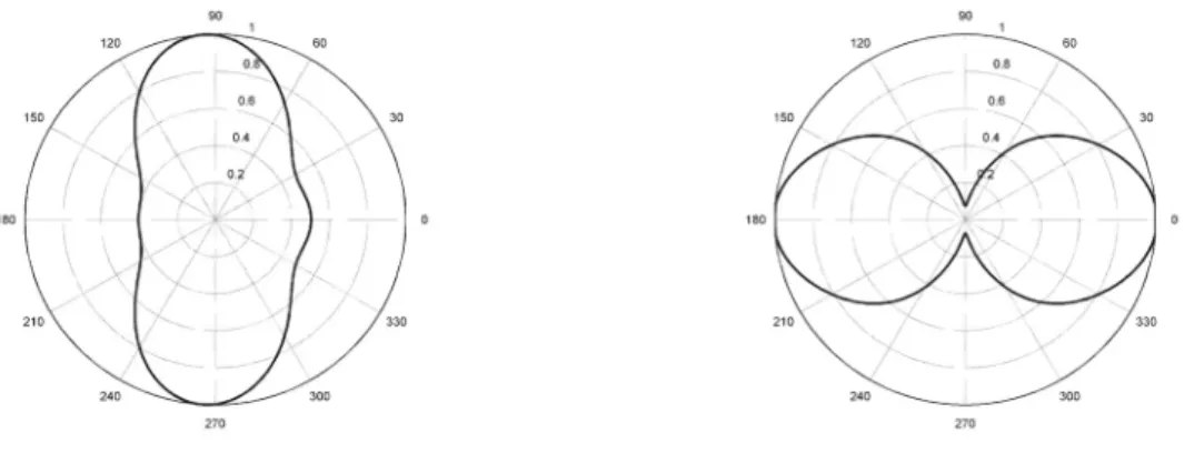
Figure 1 shows the horizontal and the vertical ra-diation diagrams based on an analytical approx-imation of damping factor functions for antenna 1. Figure 2 shows the same data for antenna 2.
a. horizontal radiation diagram b. vertical radiation diagram
Figure 1.Horizontal and vertical radiation diagrams based on an analytical approximation of a damping factor functions for antenna 1.
a. horizontal radiation diagram b. vertical radiation diagram
Figure 2.Horizontal and vertical radiation diagrams based on an analytical approximation of a damping factor functions for antenna 2.
a.antenna 1 b. antenna 2
Spatial radiation diagram for both antenna con-figurations are approximated according to[13]:
F(ϕ,ϑ)≈fh(ϕ)·fv(ϑ) (4)
Figure 3 shows spatial radiation diagrams for both antenna configurations based on equation
(4).
Strength of the electromagnetic field in three-dimensional space has been observed, so the equation for it is:
E= 5.5·
√ EIRP
(x−x0)2+ (y−y0)2+ (z−z0)2
·F(ϕ,ϑ)
(5)
where:
x0, y0 andz0 are coordinates of the transmitter
location.
Optimal transmitter parameters (power, posi-tion, azimuth and elevation) have been deter-mined using a genetic algorithm. Program MATLAB version 7.11.0.584 (R2010b) with Global Optimization Toolbox version 3.1 has been used for this purpose [14]. Fitness func-tion which needs to be minimized is:
f =min(E) +E+Ek (6)
where:
min(E)– minimal total strength of the electro-magnetic field in the whole observed area, E – mean strength of the electromagnetic field in the whole observed area,
Ek – mean strength of the electromagnetic field
in the restricted subareas.
Fitness function (6) is original and was ob-tained empirically(the authors tried several dif-ferent fitness functions and decided that this one has the best features for investigated prob-lem). Fitness function mentioned above has been used for genetic algorithm population’s individuals which satisfied the criteria of max-imal (Emax = 10V/m, for restricted subareas)
and minimal (Emin = 0.1V/m, for signal
re-ception) strength of the electric field. If a GA individual did not satisfy these criteria then its fitness function was multiplied by penalty factor of 1000.
Representation of an individual is a 6 compo-nents vector of real numbers:
v = [ERP x0 y0 z0 ϕ0 ϑ0]. Genetic algorithm
parameters are shown in Table 1. Parameters were obtained empirically (the authors tried a variety of parameter values and decided that these where the most suitable for investigated problem). In this paper the stochastic univer-sal sampling is used as a selection procedure
[15,16,17]. In each generation 4 individuals have been created with a crossover procedure, 4 individuals have been created with a mutation procedure, and 2 individuals are elite individu-als(individuals with the lowest value of a fitness function from the last generation)in each of the three subpopulations.
Parameter Value / Property
30(3 subpopulations Population size of 10 individuals) Number of generation 50
Selection Stochastic uniform Crossover Heuristic
Mutation Adaptive feasible Fitness scaling Proportional Number of elite individuals 2
Crossover fraction 0.5
Table 1.Genetic algorithm parameters in Global Optimization Toolbox.
3. Results and Discussion
To verify the method, seven cases with a differ-ent number, size and shape of restricted sub-areas were chosen (maximal strength of the electric field was Emax = 10V/m and minimal
strength of the electric field regarding signal covering wasEmin = 0.1V/m). Procedure was
1. Data represents transmitter power ERP, trans-mitter location(x0,y0, z0), horizontal direction (azimuth) ϕ0, vertical direction(elevation) ϑ0
and fitness function valuef. In Table 3 the same is presented for antenna 2.
Duration of computation for optimization pro-cedure for antenna 1 was between 171 and 173 minutes for cases from 1 to 7, and for antenna 2 it was between 167 and 178 minutes.
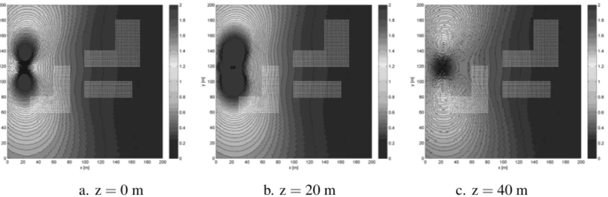
In following figures example of some results are presented. Contour and values of strength of the electromagnetic field in the whole observed area for the best individual are presented for various cases of the restricted subareas configuration. In Figure 4, contour and values of strength of the electromagnetic field in the observed area for the best individual for the 5th case of
re-stricted subarea configuration for antenna 1 and for 0 m, 20 m and 40 m heights. In Figure 5, the same is shown for the best individual for the 7th case of restricted subarea configuration. In
Figure 6, contour and values of strength of the electromagnetic field in the observed area for the best individual for the 5thcase of restricted
subarea configuration for antenna 2 and for 0 m, 20 m and 40 m heights. In Figure 7, the same is
shown for the best individual for the 6thcase of restricted subarea configuration.
In real world applications, available transmitter locations are restricted and it may not be possi-ble to place transmitter on the positions deter-mined by the best individual from a GA run. In such a case it is possible to choose one of the other “good“ individuals from a GA run. This may not be the best set of transmitter parameters
(a GA individual), but still good enough regard-ing initial conditions. Figure 8 shows examples of transmitter positions(a GA individuals from the last generation)for the 5thand the 7thcases
of restricted subarea configuration for antenna 1, while Figure 9 shows those for the 5th and the 6thcases of restricted subarea configuration for antenna 2. Figures present observing area, restricted subareas and valid transmitter posi-tions. Possible transmitter positions are marked with dark gray circles.
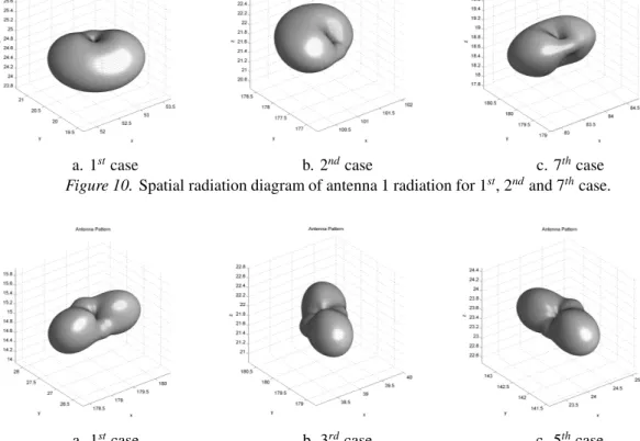
Figures 10 and 11 show examples of different spatial orientation of antennas 1 and 2 respec-tively. Figures also depict approximated spatial radiation diagrams for each antenna.
Case ERP (dbW) x0(m) y0(m) z0(m) ϕ0[◦] ϑ0[◦] f
1st 21,03 52,70 20,33 24,78 117,38 -21,15 0,73 2nd 19,65 101,09 177,68 21,65 243,32 19,60 0,90 3rd 21,40 22,83 41,25 24,26 116,17 -26,21 0,83 4th 18,96 20,83 100,86 21,86 187,21 0,73 0,84 5th 19,54 150,34 57,26 21,43 77,06 29,98 0,90 6th 18,29 164,85 22,63 20,30 358,14 3,09 0,83 7th 19,74 83,78 179,98 18,75 265,08 -22,09 0,83
Table 2.The best individuals from the last generation for a minimal strength of the electric fieldEmin=0.1V/mfor antenna 1.
Case ERP (dbW) x0(m) y0(m) z0(m) ϕ0[◦] ϑ0[◦] f
1st 22,11 179,34 27,21 14,96 265,74 28,11 1,02 2nd 21,50 20,27 33,25 27,36 135,67 7,39 0,96 3rd 20,60 39,00 179,73 21,82 210,36 -22,34 0,85 4th 19,95 163,51 45,72 21,64 77,77 24,37 1,05 5th 20,62 24,13 142,41 23,48 359,72 24,91 1,03 6th 20,77 21,57 118,53 14,17 181,29 -0,16 1,10 7th 19,38 26,48 24,69 18,61 288,46 12,98 0,90
a. z=0 m b. z=20 m c. z=40 m
Figure 4.Contour and values of strength of the electromagnetic field in the observed area for the best individual for the 5thcase of restricted subarea configuration, antenna 1, for 0 m, 20 m and 40 m heights.
a. z=0 m b. z=20 m c. z=40 m
Figure 5.Contour and values of strength of the electromagnetic field in the observed area for the best individual for the 7thcase of restricted subarea configuration, antenna 1, for 0 m, 20 m and 40 m heights.
a. z=0 m b. z=20 m c. z=40 m
Figure 6.Contour and values of strength of the electromagnetic field in the observed area for the best individual for the 5thcase of restricted subarea configuration, antenna 2, for 0 m, 20 m and 40 m heights.
a. z=0 m b. z=20 m c. z=40 m
a. the 5thcase b. the 7thcase
Figure 8.Examples of valid transmitter positions from the last generation for the 5thand the 7thcases of restricted subarea configuration for antenna 1.
a. the 5thcase b. the 6thcase
Figure 9.Examples of valid transmitter positions from the last generation for the 5thand the 6thcases of restricted subarea configuration for antenna 2.
a. 1stcase b. 2ndcase c. 7thcase
Figure 10.Spatial radiation diagram of antenna 1 radiation for 1st, 2ndand 7thcase.
a. 1stcase b. 3rdcase c. 5thcase
4. Conclusion
Based upon previous investigations[6,7,8,9]and here obtained results for two antenna types and various terrain configurations, it can be con-cluded that the method is promising and can give satisfactory results. Although the method is quite computing demanding comparing to 2D problems [6,7,8], it is still quite acceptable for ordinary and inexpensive equipment(office PC). The main reason for excessive computing requirements is the number of points in the 3D for which electromagnetic field strength has to be calculated. Aside from that, the method is simple, straightforward and independent of ter-rain configuration or antenna type. Additional method benefit are “almost” optimal solutions which give certain freedom in antenna place-ment and avoidance of prohibited placeplace-ment po-sitions for the antenna. Future investigation will include more than one antenna, where antennas can be of different types, few antennas can be positioned in the same point in 3D(on the same support pole)etc.
References
[1] E. ALBA, J. F. CHICANO, Evolutionary Algorithms in Telecommunications, http://neo.lcc.uma. es/staff/francis/pdf/melecon06.pdf,
Ac-cessed: 23.11.2011.
[2] E. ALBA, Evolutionary Algorithms for Optimal Placement of Antennae in Radio Network De-sign,http://www.lcc.uma.es/∼eat/pdf/ ni-disc2004.pdf, Accessed: 23.11.2011.
[3] E. ALBA, G. MOLINA, F. CHICANO, Optimal Placement of Antennae using Metaheuris-tics,http://neo.lcc.uma.es/staff/francis/ pdf/nma06.pdf, Accessed: 23.11.2011.
[4] S. P. MENDES, J. A. G. PULIDO, M. A. V. RO -DRIGUEZ, M. D. J. SIMON, J. M. S. PEREZ, A Differential Evolution Based Algorithm to Op-timize the Radio Network Design Problem,
http://www.icsi.berkeley.edu/∼storn/ deb06.pdf, Accessed: 23.11.2011.
[5] A. J. NEBRO, E. ALBA, G. MOLINA, F. CHICANO, F. LUNA, J. J. DURILLO, Optimal Antenna Placement Using a New Multi-Objective CHC Algorithm,
http://neo.lcc.uma.es/staff/guillermo/ index files/files/MOCHC.pdf, Accessed:
23.11.2011.
[6] T. ROLICH, D. GRUNDLER, Minimizing Environ-mental Electromagnetic Field Pollution Adjusting Transmitter Parameters Using Genetic Algorithm,
2009 IEEE Congress on Evolutionary Computation, Trondheim, Norway, pp. 881–887,(2009).
[7] T. ROLICH, D. GRUNDLER, Managing Electromag-netic Field Pollution Using GeElectromag-netic Algorithm,
32nd International Convention on Information and Communication Technology, Electronics and Mi-croelectronics – MIPRO 2009, Opatija, Croatia, pp. 227–232,(2009).
[8] T. ROLICH, D. GRUNDLER, Determining optimal power, location and direction of transmitters using a genetic algorithm, 33rdInternational Convention
on Information and Communication Technology, Electronics and Microelectronics – MIPRO 2010, Opatija, Croatia, pp. 161–166,(2010).
[9] T. ROLICH, D. GRUNDLER, Reduction of electro-magnetic field pollution in 3D space using a ge-netic algorithm, 2010 IEEE World Congress on Computational Intelligence, Barcelona, Spain, pp. 3945–3949,(2010).
[10] CEI/IEC 61566: 1997 International Standard: Measurement of exposure to radiofrequency elec-tromagnetic fields – Field strength in the frequency range 100 kHz to 1 GHz, 1997.
[11] Kathrein Scala Division – professional antenna and filter products for broadcast, land mobile and wireless communication applications, Available:
http://www.kathrein-scala.com/, 2011.
[12] The MathWorks – MATLAB and Simulink for Technical Computing, Available:
http://www.mathworks.com/, 2011.
[13] F. MIKAS, P. PECHAC, The 3D Approximation of Antenna Radiation Patterns, The Institute of Elec-trical Engineers, The IEE, Michael Faraday House, Six Hill Way, 2003.
[14] Genetic Algorithm and Direct Search Toolbox User’s Guide, Version 2, The MathWorks, Inc., 2006.
[15] J. E. BAKER, Reducing Bias and Inefficiency in the Selection Algorithm,Proceedings of the Second In-ternational Conference on Genetic Algorithms and their Application, pp. 14–21, 1987.
[16] T. B ¨ACK, Evolutionary Algorithms in Theory and Practice: Evolution Strategies, Evolutionary Pro-gramming, Genetic Algorithms, Oxford University Press, 1996.
[17] D. E. GOLDBERG,Genetic Algorithm in Search, Op-timization and Machine Learning, Addison-Wesley, Reading MA, 1989.
Contact addresses: Tomislav Rolich Faculty of Textile Technology University of Zagreb, Croatia e-mail:[email protected] Darko Grundler Faculty of Textile Technology University of Zagreb, Croatia e-mail:[email protected]
TOMISLAVROLICHwas born on 22ndApril 1971 in Zagreb. He
gradu-ated from the Faculty of Electrical Engineering and Computer Science, University of Zagreb in 1995, under the mentorship of Prof. Neven Mijat.
In January 1995, during the study, he got a job in the Technical School “Ruder Boˇskovi´c”, first as an associate and later as a teacher. In October 1998 he got a job at the Faculty of Textile Technology, University of Zagreb as a junior assistant for the courses: Information, Computing and Applied Computing. At the same time he enrolled in postgraduate studies at the Faculty of Electrical Engineering and Computer Science, University of Zagreb.
In November 2001, he got the Master’s degree from the Faculty of Elec-trical Engineering and Computer Science, University of Zagreb, with the theme “Evaluation of the Application of Evolutionary Algorithms in Achieving Optimal Control” under the mentorship of Prof. Darko Grundler. In April 2005 he got the Ph.D. degree from the Faculty of Electrical Engineering and Computer Science, University of Zagreb, with the theme “Searching the Space of Aesthetic Evaluation for Match-ing Weave and Color in Fabrics Design” under the mentorship of Prof. Darko Grundler.
His research activity is in technical sciences, computer engineering and artificial intelligence and his area of special research interest is evo-lutionary algorithms, neural networks and fuzzy logic. His current position is that of an associated professor at the Faculty of Textile Tech-nology, University of Zagreb. He has published 39 papers, delivered 15 presentations at international conferences; he is co-author of several university handbooks and two university textbooks.