Regularized SVM Classification with a new Complexity-Driven Stochastic Optimizer

Regularized SVM Classification with a new Complexity-Driven

Stochastic Optimizer

J. Andrew Howe

_{, Hamparsum Bozdogan}

2_{KAPSARC, Riyadh, Saudi Arabia (affiliated after article accepted)}

3_{University of Tennessee, Department of Business Analytics & Statistics, Knoxville, Tennessee, USA}

Abstract. Given a multivariate dataset composed of data from different known sources or processes, how can we create a rule to separate the data, and classify any future data? Kernel discriminant analysis is one of many supervised learning techniques that handle this problem. Recently, in this and other knowledge discovery problems, kernel methods have gained popularity. This is somewhat ironic as another common theme is variable reduction, and kernel methods actually inflate dimensionality. Due to the substantial benefits of processing "kernelized" data, this is excusable - kernel methods frequently outperform traditional classification techniques for real data when the classes are not easily separable. In performing kernel discriminant analysis, there are two main issues that we address in this article. The first is that, in the literature, the question of which kernel function to use is often subjectively selecteda prior, or determined by cross-validation with the sole objective of maximizing classification performance. Secondly, after obtaining discriminant functions or support vectors to classify a dataset, how do we know which of our variables are most responsible for, and important to, the classification? In this research, we develop a new regularized algorithm that simultaneously selects the kernel function and subset of original variables. Our algorithm, a hybrid of cross-validation and the genetic algorithm, does this by optimizing a function that rewards correct classification while penalizing model complexity and misclassification.

We report results on three real datasets, including data from a medical imaging study. For the latter, we obtained an impressively low misclassification rate of 0.3%, while reducing the number of features fromp=20 to p∗=6.

2010 Mathematics Subject Classifications: 62H30, 68T10

Key Words and Phrases: Supervised classification, Discriminant analysis, Support vectors, Information criteria, Feature selection, Stochastic optimization, Reproducing kernel Hilbert space, Machine learning

∗_{Corresponding author.}

Email addresses:[email protected](J. Howe),[email protected](H. Bozdogan)

http://www.ejpam.com 216 c 2016 EJPAM All rights reserved.

Vol. 9, No. 2, 2016, 216-230

1. Introduction

Logistic regression is a well-known form of nonlinear regression in which responses can take on values of 0 or 1 (or any binary format). From a different perspective, we can see the binary responses as class labels for data from two groups. This leads us to the concept of discriminant analysis, which is closely related to logistic regression. In general, the goal of discriminant analysis is to determine data groupings that minimize the variability within the groups and maximize the variability between the groups. Differently put, given known class labels for the data, the goal is to minimize the probability of misclassification - it is a method ofsupervised learning. When we perform kernel discriminant analysis (KDA), this does not change. To use kernel discriminant analysis, one merely has to apply a kernel function to the data, then perform the usual analysis. This does, however, present two issues which we address in this research.

• There are many possible kernel functions that can be applied to perform the nonlinear map into higher-dimensional feature space. The choice of the kernel function can have a substantial impact on the analytical results. For example, use of a linear kernel on data that is inherently nonlinear will likely inflate the classification error. For univariate or bivariate data, it may be easy to determine nonlinearity, but what of ten variables? In most relevant research with kernel methods, the kernel function is either selecteda priorior using cross-validation to minimize the testing classification error. How do we choose the "best" kernel function consistent with the principal of Occam’s Razor?

• For any classification method, there is often value in knowing which variables contribute most to the separation of the classes. Of course, this is generically true about all statistical data mining/ machine learning techniques. However, with kernel methods, after we apply the kernel function, it is impossible to perform any meaningful feature selection analysis. Perhaps we are making ten hopefully predictive, and costly, measurements on a process but we can get very low classification errors only using three of them? Why take unnecessary measurements for a model that is overly complex when we can have a model that is both accurate and parsimonious? How do we determine which variables are contributing the most to our discriminant functions in the kernel space?

2. Regularized Kernel Discriminant Analysis with Support Vectors

2.1. Kernels

Reproducing Kernel Hilbert Spaces were initially developed by the mathematician Aron-szajn[2]. Assuming they meet Mercer’s conditions, kernel functions correspond to a nonlinear map into a higher dimensional feature spaceF_{and then taking the dot product in this space.} As an example, consider the mapφ:R2→R3_{, defined asφ}€_x1,x2′Š_=x2

2,

p

2x₁x₂,x2₂′. For two vectors xi andxj, we have

φ xi

′

φ xj

=”x2_i2,p2xi1xi2,x2i2

— ”

x2_j2,p2xj1xj2,x2j2

—′

=”x2_i2x2_j2, 2x_i1xi2xj1xj2,x2i2x 2

j2

—

= x′_ixj

2

This last equality is called the quadratic kernel (with no intercept), which we may denote as K xi,xj

; by computing the quadratic kernel function, we avoid performing the map. This is called thekernel trick. For a datasetx withnrows andpvariables, the data is translated into a square matrix of sizenin the feature space, in which every possible pair of points is evaluated. Note that this translation is neither one-to-one, nor onto - application of a kernel function is an non-invertible process. Once the data has been classified in the feature space, we have no way to go back to the original data space and judge the value of individual variables.

Petal Length

Sepal Width

(a) Iris Data (b) 1st_{two Variables after Kernel Trick}

Figure 1: Demonstrating Separation in Kernel Space; x is Setosa, o is Versicolor, and _∗ is

Virginica.

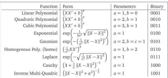
The set of kernel functions which we use in this research is composed of the nine most com-mon, as listed in Table 1. For each kernel, we indicate the parameters we used. It is generally

Table 1: Kernel Functions Available.

Function Form Parameters Binary

Linear Polynomial X X′+ba a=1,b=0 0001 Quadratic Polynomial X X′+ba a=2,b=1 0010 Cubic Polynomial X X′+ba a=3,b=1 0011

Exponential exp

− 1 2a2

Æ

kX−Xk2

a=1 0100

Gaussian exp€− _a1bkX−Xk

2cŠ _{a=2,b=c=1 0101}

Homogenous Poly. (homo) _a12X X′

b

a=1,b=2 0110

Laplace exp

−q1

a2kX−Xk

2

a=1 0111

Cauchy 1+1_akX−Xk2−1 a=1 1000

Inverse Multi-Quadric kX−Xk2+a2−

1

2 _{a=1 1001}

2.2. Binary Discriminant Analysis

Our data x is composed ofnrealizations ofpcontinuous measurements. Accompanying X is a vector of class assignments y ∈[1, 2]. Having y_i =1 indicates that x_i is an element of the first group. After mapping the data into the feature spaceF_{, the goal is to find a direction}

ψ=

n X

i=1

α_iφ x_i=α,x_i (1)

with weight vectorαthat maximizes the Fisher criterion

JF(α) =

α′Σˆ_Bα

α′Σˆ_Wα. (2)

ˆ

Σ_Bindicates thebetween-group covariance matrix, and ˆΣ_W is thewithin-group covariance ma-trix, shown in (3) and (4), respectively.

ˆ

Σ_B= x1−x2

′

x1−x2

(3)

ˆ

Σ_W =1 nW =

1 n

2

X

k=1

I_y

i=k x−xk

′

x−x_k (4)

x_k is the mean of observations belonging to classk, and I_y=k is an indicator function which

takes on the value 1 when the specific datapoint is in groupk(0 otherwise). The binary kernel discriminant function and classifier are:

f x_i=α,K x_i,x+b, and (5)

q x_i=

¨

1 f xi

≥0

2 f x_i<0. (6)

where the vectorαis obtained by solving (2), andbis the intercept of the separating hyper-plane, which passes through the midpoint of the class centroids.

2.3. Binary Support Vectors

Generalizing this further, we can rewrite (5) as

f xi

=α∗,ks xi

+b∗,

wherek_s x_i=K x_i,s₁,K x_i,s₂, . . . ,K x_i,s_mis the vector of theithdatapoint evaluated at themsupport vectors, which form a subset of the data. This is thesupport vector machine (SVM). Thus, optimization of the weights and intercept becomes the quadratic programming problem shown here.

(α∗,b∗) =min

α,b

–

1 2kαk

2_+C

n X

i=1 ξd_i

™

α,x_i+b≥1−ξ_i,i∈I₁,

α,x_i+b≤ −1+ξ_i,i∈I₂,

C >0,ξ_i≥0,i∈I₁[I₂

Whend =1, we say the SVM isL1 soft margin trained, otherwise, it’sL2 soft margin trained. C is a regularization constant, andI₁ andI₂ are slack variables used to relax the inequalities for non-separable data.

2.4. Multi-class SVM

For data composed ofK>2 classes indexed byk, we consider a set of discriminant func-tions

f_k x_i=α_k,k_s x_i+b_k.

There are several ways to decompose the multi-class SVM, includingOne-Against All (OAA) andOne-Against-One (OAO)- see[11].

The OAA decomposition works by trading the single multi-class problem forKbinary SVM problems, where the binary state vector y_k′ is

y_k′=

¨

1 for y = y_k

2 for y 6= yk

.

For example, if we hadK=4 classesA,B,C, andD, OAA would solve four binary problems:

AvsBCD, BvsACD, CvsABD, DvsABC

The multi-class classification rule used is then

q x_i= max

k=1,2,...,Kfk xi

. (7)

OAO, on the other hand, solves the multi-class problem by solving K′ = K(K₋1)/2 binary SVM problems, in which all pairs of classes are considered. The majority voting strategy shown in (8) is used to select the final class assignments. The vector vote x_iindicates the frequency with which, from allK′binary SVM results, the ith datapoint was classified into each group.

vote xi

=v1 xi

,v2 xi

, . . . ,vK′ xi

q xi

= max

y_i′=1,2,...,K′vot e xi

₍₈₎

Using the same groupsA,B,C, andD, OAO solves the six binary SVMs

2.5. Hybridized Covariance Estimation

In broad terms, KDA means applying the appropriate calculations in Sections 2.2 through 2.4 after application of the kernel trick. When performing KDA, it can be usually expected that the within-group covariance matrix (4) won’t be nonsingular or positive definite. Singularity of this kernel covariance matrix is a problem that has attracted many researchers, and many methods have been proposed to make the matrix well-conditioned. In [12], Liberati et al. introduced a hybridized covariance estimator ˆΣ_{S TA_C S E} that joins the stabilization technique of Thomaz [15] with theconvex sum covariance estimator shrinkage technique of press [14]

and Chen[6]. There is an optional third step, which we apply to help regularize especially sparse and / or singular matrices. After computing the hybrid stabilized kernel matrix, we compute its singular values. ˆΣ_{S TA_C S E}is then replaced with a diagonal matrix of some subset of the largest singular values as areduced rank approximationΣˆ∗_{S TA_C S E}. For the real datasets analyzed in this research, we kept the top 25 when further regularization was necessary.

3. Cross-Validation Genetic Algorithm for Optimization

The Genetic Algorithm (GA) is a stochastic search algorithm that borrows concepts from biological evolution[7–10]; it has been used successfully in a wide range of statistical mod-eling applications. The solution space for a problem is explored via an ensemble of strings which represent possible solutions. In the parlance of the GA, these solution strings are called chromosomes. Chromosomes are created by encoding solutions using a fixed, finite-length al-phabet of symbols. Solutions for the GA are most typically coded as binary strings. Individual chromosomes are allowed to compete with each othera lanatural selection, to create better solutions, with the goal to optimize some objective function. Operational details of the GA can be found in the above-mentioned sources, or any number of others.

For the problem of selecting a subset of p variables, a chromosome is a p-length vector such that each element represents the presence (1) or absence (0) of a specific variable. An example chromosome may be[10011001]; in this case, predictors 1,4,5,8 are selected while 2,3,6,7 are not. Our algorithm uses the GA to simultaneously determine the best subset of variables AND the best kernel function. We do this by coding the different kernel functions into a binary string, and appending this onto the feature selection string.

We have 9 kernels to choose from; 9 in binary representation requires 4 bits. Hence, the kernels are represented by binary strings from[0000](linear polynomial) to[1001](inverse multi-quadric). The allowed kernel binary codes are shown along with the kernel functions in Table 1. An obvious issue is that four binary digits can be used to represent all the counting numbers up to fifteen, and yet we only have nine kernels. Hence, the GA’s crossover and mutation operators can both generate illegal strings representing kernels that we don’t have.

be have any systemic effect.

Hence, a chromosome in our algorithm is ap+4-length binary string representing a specific subset of features and kernel function. The genetic algorithm is allowed to progress for twenty generations, operating on an ensemble of twenty of these solutions, with the goal to minimize the objective function I COM P_{P ERF}.

3.1. Information Complexity Criteria for Supervised Classification

A logical next step from information theoretic model selection criteria such as Akaike’s AIC and Schwartz’s SBC, Bozdogan introduced and developed his information complexity criteria I COM P in [4, 5, (and others)]. I COM P typically penalizes models based on the maximal entropic complexity C₁ of the model covariance matrix [3], as opposed to functions of the number parameters estimated. This penalty allowsI COM P, shown in (9), to simultaneously penalize a model based onlack-of-fit,lack-of-parsimonyandprofusion-of-complexity.

I COM P(_Fˆ−1_{) =−2 logL(θˆ|X)} lack-of-fit

+2C1(Fˆ−1)

compl e x i t y

(9)

Several versions of I COM P have been developed for various model selection problems. For the problem of kernel-based supervised learning, Liberatiet al. [12]introduced I COM P_{P ERF}. This form ofI COM P is conceptually based on the regression-basis of discriminant analysis:

I COM P_{P ERF} =nlog 2π+nlog ˆσ2+n

| {z }

l ack−o f−f i t

+2C_1F€Σˆ∗_{S TA_C S E}Š

| {z }

compl e x i t y

, (10)

where ˆσ2 = 1_nPn_i=1 y_i−yˆ_i2. The y_i are the actual known group labels, and the ˆy_i are the group labels predicted with KDA. The kernel methods used in KDA lead to orthogonal and highly sparse matrices, which can cause problems for theC1 measure of complexity. Ac-cordingly, I COM P_{P ERF} uses a modified measure of complexity based on theFrobenius norm characterization of the entropic complexityC_F, shown in (11) as a function of the eigenvalues of the matrix.

C1F(·) =

1

4λ2

p X

i=1

€

λ_i−λŠ2 (11)

By minimizingI COM P_{P ERF}, our algorithm can simultaneouslyminimize classification error,

maximize fit, andminimize model complexity.

3.2. Cross-Validation within the GA: CVGA

To avoid bias due to the randomized partitioning, we could run the GA many times (called replications), each time with a new CV sample, but it would be very time consuming to do this on top of the GA. At the end, we’d need to combine the results from all the replications to determine the optimal model. Instead, we propose a hybrid algorithm that combines the GA with cross-validation, calledCVGA. CVGA adds an extra layer of randomness to the GA in that every time the fitness of a chromosome is evaluated, it is based on a new cross-validation sample. Instead of nesting the GA within CV, CV is nested within the GA. This allows us to score solutions during optimization with no concern that our partitioning into training/testing for the GA was somehow not representative. However, the extra randomness within the CVGA does present a challenge.

Suppose in one iteration of the CVGA, we find the best solution to use variables 1 and 2 and the Gaussian kernel, with a score of₋67. In a later generation, the same solution could result in a score of −23, and not be the best for that iteration. This variability is obviously due to the fact that the fitness of each chromosome is evaluated on different data. We have implemented a two-stage process to smooth out this variation.

First, in summarizing the results from the GA, we store the medianI COM P_{P ERF}and testing

/training classification error rates for every unique solution (since good solutions will tend to be occur multiple times). The median is used instead of the average to ensure that the optimal solution selected at the end of the process is robust against cross-validations with outlying performances. Secondly, we actually run the GA 100 times, for a maximum of 100×20× 20=40, 000 unique solutions evaluated. The medianI COM PP ERF for each solution evaluated

is then averaged over all 100 replications, and we compute the 95% empirical confidence intervals for the misclassification rates.

In summary, computing the fitness for each chromosome follows these steps:

(i) randomly partition the data into training and testing sets, keeping only the features selected by the chromosome

(ii) perform KDA on the training set, measuring the classification error, and the complexity of the reduced rank hybrid stabilized kernel matrix; this is for the complexity term of I COM P_{P ERF} in (10)

(iii) use the KDA model to classify the data in the testing set, measuring the classification error, and the negative maximized likelihood; this is for the lack-of-fit term in (10)

(iv) join the two parts of I COM P_{P ERF} together

4. Numerical Results

4.1. X-ray Burst Event Data

withn₁=132 observations, and the second with the remainingn₂=42. Table 2 displays the four unique solutions chosen across by the CVGA.

Table 2: Models Selected for the X-ray Burst Data.

Subset Kernel I COM P_{P ERF} Training Err. CI Testing Err. CI GA. Freq. {1, 2_} Laplace -77.78 [0.00, 0.00] [0.72, 0.72] 86 {1, 2} Exponential -71.81 [0.00, 0.00] [0.57, 0.89] 10 {1, 2} Inv. Multi-Quadric -55.2 [0.00, 0.00] [0.33, 1.29] 1

{1_} Laplace 9.12 [0.00, 2.62] [0.45, 2.33] 3

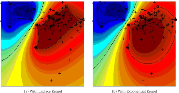
Not only was the best solution selected by 86% of the replications, more than half of the total generations selected it. Using the Laplace kernel function on both variables of this data is a very clear winner with a 0.72% probability of misclassification, not that any of these four models had unreasonable error rates. Figure 2 has the scatter plots plus the contours for the top two solutions. Note the clear separation boundary between each group - hence the low misclassification rates are not unexpected. Both models used a small number of support vectors - 14 and 11, respectively. Less than 10% of the observations was needed, which shows the efficiency of support vector classification. Clearly the full GA with cross-validation model was overkill for this dataset, as complete enumeration would only need to evaluate 27 solutions. It has been included here purely for the visualization the support-vector-based separation areas, which will not be possible for the other examples.

(a) With Laplace Kernel (b) With Exponential Kernel

4.2. Wine Composition Data

Our next example is the wine recognition dataset of M. Fiorina,et al., used in[1]. These data are the results of a chemical analysis of n = 178 wines grown in the same region in Italy but derived from K = 3 different cultivars (n1 =59, n2 =71, n3 = 48). The analysis determined the quantities ofp=13 chemical constituents found in each of the three types of wines. The variables are shown in Table 3.

Table 3: Wine Data Variables.

Variable Variable

x₁ Alcohol x₈ Non-flavonoid Phenols x2 Malic Acid x9 Proanthocyanins

x3 Ash x10 Color Intensity

x₄ Alkalinity of Ash x₁₁ Hue

x5 Magnesium x12 OD280/OD315 of Diluted Wines

x6 Total Phenols x13 Proline

x₇ Total Flavonoids

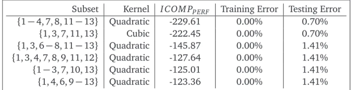
With this dataset, there are 9× 213−1=73, 719 possible nontrivial solutions; the CVGA with 100 replications of the GA explored nearly half of the solution space. None of the gener-ations selected the saturated model with all features as the best; the most frequently selected kernel functions were the Quadratic (25%) and Exponential (18%). In Table 4, we report the best 6 models with their classification results. The top 6, as opposed to a round number, were chosen, since they had identically perfect training errors.

Table 4: Top 6 Models Selected for Wine Data.

Subset Kernel I COM PP ERF Training Error Testing Error

{1−4, 7, 8, 11−13} Quadratic -229.61 0.00% 0.70% {1, 3, 7, 11, 13} Cubic -222.45 0.00% 0.70% {1, 3, 6−8, 11−13} Quadratic -145.87 0.00% 1.41% {1, 3, 4, 7, 8, 9, 11, 12} Quadratic -127.64 0.00% 1.41% {1−3, 7, 10, 13} Quadratic -125.01 0.00% 1.41% {1, 4, 6, 9−13} Quadratic -123.36 0.00% 1.41%

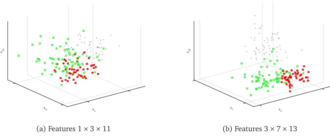
In Figure 3, we show 3-way scatterplots for two of the possible ten combinations of these five variables. The plots selected were fairly representative of all 10 - there were no 3-way plots with clear separation of all classes in the original data space. This suggests that the kernel methods boosted classification performance as we expect.

x1 x

3

x11

(a) Features 1×3×11

x3 x

7

x13

(b) Features 3×7×13

Figure 3: Trivariate Grouped Scatterplots for the Best Wine Subset.

4.3. Aorta Nuclear Resonance Image Data

Our final example is by application to medical imaging data from a study of heart tissue. Hardening of the arteries is a leading cause of death and debility in the industrial world. In the U.S. alone 13 million Americans suffer from heart attacks, and 90, 000 people die from heart disease annually. Nuclear Magnetic Resonance (NMR) imaging has been used to aid clinical identification of fatty tissues in the arteries to aid in early detection of heart attacks. The aorta data analyzed here was collected by Pearlman [13] at the Medical School of the University of Virginia. There are observations from n= 418 patients on 16 different image acquisition variables. Including direction and orientation variables, we havep=20 variables. The first n1 = 194 patients exhibited early atheroma, and the remaining n2 = 224 patients were clinically deemedhealthy.

For this dataset which exhibits marked non-normality, there are 9, 437, 175 possible sub-set+kernel combinations. The CVGA ran 100 replications of the genetic algorithm, with each running for twenty generations with a population size of twenty-five. With the elitism rule turned on, our modeling process evaluatedat most 69, 000 unique solutions - 0.73% of the solution space.

Before running the full modeling procedure, we performed some exploratory data analy-sis using the full set of features. In this analyanaly-sis, we generated 100 training/testing cross-validation samples, and fit each of the 9 kernels to all. With the full dataset, the 95% confidence interval of the testing error rates with the Cauchy was abysmal: [43.80%, 47.65%]. This once again demonstrates the clear benefit of optimal feature selection.

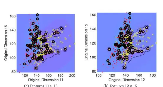
Table 5 show five of the best models. While the Cauchy kernel appears superior for this data, it seems there is no clear best set of features, since all of the top five performed nearly perfectly. The top model with the Cauchy kernel has dramatically reduced the dimensionality of the data, from p=20 variables down to p∗=6. Figure 4 displays the poor separation in the original data space for two sets of pairs of the original features.

Table 5: 5 of the Best Models Selected for Aorta Data.

Subset Kernel I COM P_{P ERF} Training Error Testing Error {5, 7, 8, 11, 12, 15} Cauchy -530.05 0.00% 0.30% {4, 5, 8, 9, 11, 16, 18} Cauchy -530.05 0.00% 0.30% {4, 7−9, 11−13, 15, 18} Linear -440.22 0.00% 0.30% {3,−5, 7, 9, 12−16, 19} Cubic -145.87 0.00% 0.30% {2−7, 9, 10, 12, 14, 15, 17, 19} Homogenous Poly -127.64 0.00% 0.30%

(a) Features 11×15 (b) Features 12×15

Figure 4: Bivariate Grouped Scatterplots for Aorta Data Showing Poor Separation.

5. Concluding Remarks

classification with kernel discriminant analysis. However, CVGA can be useful for any machine learning problem that requires cross-validation and exploration of a large solution space. The only requirement is the ability to encode solutions as GA chromosomes.

Recall that we set the kernel function parameters to certain values a priori, instead of estimating them from the data. This research could be further extended to allow estimation of the parameters. One approach might be to merge the CVGA with the data-adaptive technique presented in[12].

References

[1] S Aeberhard, D Coomans, and O de vel. Comparison of Classifiers in High Dimensional Settings. Technical Report 92-02, Dept. of Computer Science and Dept. of Mathematics and Statistics, James Cook University of North Queensland, 1992.

[2] N Aronszajn. Theory of Reproducing Kernels. InTransactions of the American Mathemat-ical Society, volume 68, pages 337–404, 1950.

[3] H Bozdogan. ICOMP: A New Model-Selection Criteria. In H H Bock, editor, Classifica-tion and Related Methods of Data Analysis, pages 599–608. Elsevier Science Publishers, Amsterdam, The Netherlands, 1988.

[4] H Bozdogan. On the Information-Based Measure of Covariance Complexity and its Ap-plication to the Evaluation of Multivariate Linear Models. Communication in Statistics, Theory and Methods, 19:221–278, 1990.

[5] H Bozdogan. Akaike’s Information Criterion and Recent Developments in Information Complexity. Journal of Mathematical Psychology, 44:62–91, March 2000.

[6] M Chen. Estimation of Covariance Matrices Under a Quadratic Loss Function. Research Report S-46, Department of Mathematics, SUNY at Albany, 1976.

[7] D Goldberg. Genetic Algorithms in Search, Optimization and Machine Learning. Addison-Wesley Longman Publishing Col, Inc.„ Boston, USA, 1989.

[8] R Haupt and S Haupt. Practical genetic algorithms. John Wiley, Hoboken, USA, 2004.

[9] J H Holland. Adaptation in Natural and Artificial Systems: An Introductory Analysis with Applications to Biology, Control, and Artificial Intelligence. The University of Michigan Press, Ann Arbor, USA, 1975.

[10] J H Holland. Genetic Algorithms. Scientific American, 267:66–72, 1992.

[11] C Hsu and C Lin. A comparison of methods for multiclass support vector machines. In IEEE Transactions on Neural Networks, volume 13, pages 415–425, 2002.

[13] J Pearlman. Nuclear Magnetic Resonance Spectral Signatures of Liquid Crystals in Human Atheroma As Basis For Multi-Dimensional Digital Imaging of Atherosclerosis. PhD thesis, University of Virginia, 1986.

[14] S Press. Estimation of a Normal Covariance Matrix. Technical report, University of British Columbia, 1975.