C-Support Vector Classification the Estimation of the MS Subgroups Classification with Selected Kernels and Parameters

Case Study Application for C-Support Vector Classification: The

Estimation of MS Subgroup Classification with Selected Kernels

and Parameters

Yeliz Karaca

_{, ¸}

_{Sengül Hayta}

_{, Rana Karabudak}

1 _{Department of Economics, Faculty of Management and Administrative Sciences,Süleyman ¸Sah} University, Istanbul, Turkey

2_{Department of Computer Engineering, Faculty of Engineering, Haliç University, Istanbul, Turkey} 3_{Department of Neurology, Faculty of Medicine, Hacettepe University, Ankara, Turkey}

Abstract. The study has classified the subgroups of Multiple Sclerosis (MS) using Support Vector Ma-chines (SVM). C- Support Vector Classifier (C-SVC) algorithm, one of the SVM classifiers of multi class, has been utilized for the classification of MS subgroups. For this purpose, 120 MS patients (76 RRMS, 38 SPMS, 6 PPMS patients) have been included in the study. Through Magnetic Resonance Imaging (MRI), the number of lesion diameter and Expanded Disability Status Scale (EDSS) data are applied through C-SVC. Lesion data has been obtained from three separate regions of the brain which are brain stem, periventricular corpus callosum and upper cervical region. By applying the data onto Radial Basis Function kernel (RBF), Polynomial kernel, Sigmoid kernel and Linear kernel, four of the kernel types of C-SVC algorithm, the accuracy rates of MS subgroups classification and the computation time during the training procedure are computed and compared. By adding EDSS score into the dataset, the classification achievement rate has increased in all the kernel types based on the analyses conducted. Having applied C-SVC on MS subgroups, classification achievement of MS subgroups, namely that of RRMS, SPMS and PPMS has been measured.

2010 Mathematics Subject Classifications: 62-07,92B05,62F07,90C99

Key Words and Phrases: C-SVC Kernels, MS Subgroups, MRI, EDSS, Classification.

1. Introduction

Multiple sclerosis (MS) is a disorder of the Central Nervous System (CNS) that affects the brain and spinal cord and is accompanied by inflammatory, demyelinating and axonal damage. CNS transmits electrical messages in different parts of our body along the nerves. Such messages have control over all of our movements, both voluntary and involuntary. MS

∗_{Corresponding author.}

Email addresses:[email protected](Y. Karaca),[email protected](¸S. Hayta), [email protected](R. Karabudak)

http://www.ejpam.com 196 c 2016 EJPAM All rights reserved.

Vol. 9, No. 2, 2016, 196-215

disorder, however, disrupts the proper transmission of these messages. The disorder causes neuronal dysfunction, bringing about the likelihood of long-term permanent damages. At the initial stage, a specific reason for the disorder is not known, thus it could be improbable to prevent and treat the disorder. In our day there exist no treatments that provide cure for MS. Yet, in the last two decades, several treatments have been developed and put into use, which reduce frequency of attacks, increase in the number of the plaques traced in MRI and permanent impairment in the long-run[22].

MS is categorized into 4 different clinical subtypes based on the attacks and existence of progression. The most frequently-seen one, called Relapsing Remitting MS (RRMS), is seen in 70% of the patients. Patients experience neurological loss during the attacks of RRMS based on the localization of the lesions. After the attack is over, the patients go through the remission phase and findings followed during the attack period are lost. About 50% of the patients of RRMS go under a progressive stage in which the attacks do not have remission in a period of 10 years. This form is called Secondary Progressive MS (SPMS). The patients afflicted by this form are observed to have accumulated neurological impairment over the years. In some patients, attacks and progression are seen in the course starting with the beginning phase of the disorder. This is a form called Relapsing Progressive MS (RPMS) in which the impairment gains a permanent state following each attack, and an accumulation of impairment is seen during the attack. In the rare form of MS, Primary Progressive MS (PPMS), attacks are not seen in the picture but similar to the case of SPMS, accumulation of neurological impairment is observed in the patients over the years. PPMS is seen in 10 - 15% of the patients, and its diagnosis is of critical importance since it is the form of MS that has the highest resistance to treatment[17, 21, 23, 26–28]. It is important that the subtypes of the disorder and their likelihood of causing disability in the future be identified in the early phase. It is also important to identify and compare the MRI lesion characteristics of the groups corresponding as well as the lesion load so that the treatment regimen can be figured out at an early stage and indicate the success of follow-up.

For the clinical diagnosis of MS disorder and its subgroups, lesion size received from the MR images of the patients taken on regular basis throughout the years and EDSS score based on McDonald criteria are used in this study[16]. The dataset is made up of data belonging to 120 MS patients.

disorder, MRI data has been used by examining the EDSS scores (the number of lesion diame-ter for three different regions identified was taken as a paramediame-ter). The multi class library of LibSVM of SVM supervised algorithm, one of the machine learning algorithms, has been used in this study for the diagnosis of the disorder for RRMS, SPMS and PPMS. Two different sets of data have been studied for the multi class SVM applying Radial Basis Function, Polynomial, Sigmoid and Linear kernels. For the first data set, using the number of each lesion diameter (width) for three different parts separately, a matrix of size 120×227 has been obtained.The second data set yields a matrix of 120x228 with EDSS scores and MRI data of 120 patients

(the number of lesion diameter/width for three different regions separately). So as to see

the significance of the parameter, EDSS score has been removed from the second dataset. C-SVC (C-Support Vector Classification) is a multiclass Support Vector Machine algorithm method. Data has been applied onto methods such as Radial Basis Function (RBF) kernel, Poly-nomial kernel, Sigmoid kernel and Linear kernel which are considered as C-SVC algorithms

[18]. According to C-SVC kernels experimental results have been given by two aspects that

are k-fold cross validation and computation time. In the meantime, performance evaluation

has been made through k-fold cross validation (k = 10). The computation time during the

classification of the C-SVC kernel (Radial Basis Function kernel, Polynomial kernel, Sigmoid kernel, Linear kernel) methods have been provided in a comparative fashion. Please see Table 2 for a brief review of relevant literature.

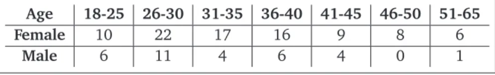
Table 1: Age Intervals Based on the Gender of the Patients in the Dataset.

Age 18-25 26-30 31-35 36-40 41-45 46-50 51-65

Female 10 22 17 16 9 8 6

Male 6 11 4 6 4 0 1

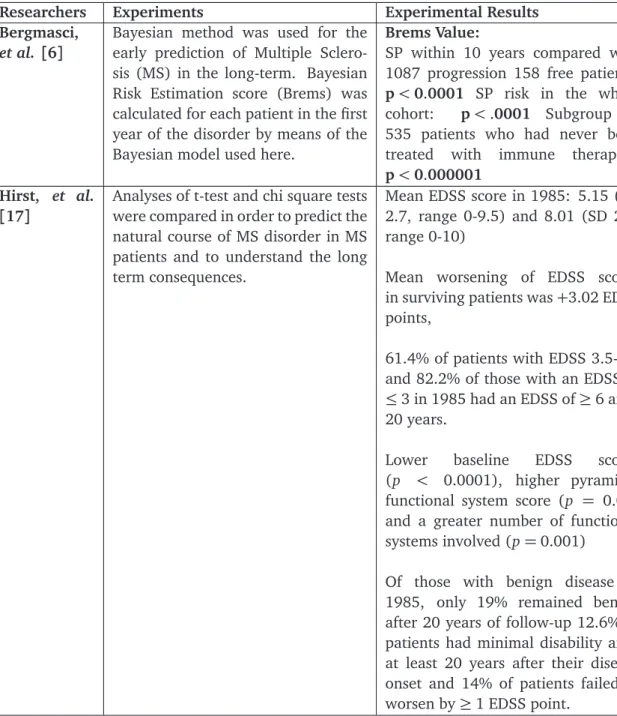
Table 2: Literature Review on MS.

Researchers Experiments Experimental Results Gutermana,

et al_[14]

Data concerning 100 MS patients and control group with 100 individuals (brainstem trigeminal) evoked po-tential data was applied to Multi-Layer Perceptron Probabilistic Neu-ral Network and Kohonen’s Learning Method diagnosing Multiple

Sclero-sis. The performance of the

neu-ral networks based classifiers is com-pared with that of the human experts and the Bayes classifier.

Kohonen Learning: 91.91%

Table 2: Literature Review on MS.

Researchers Experiments Experimental Results Bergmasci,

et al. _[6]

Bayesian method was used for the early prediction of Multiple Sclero-sis (MS) in the long-term. Bayesian Risk Estimation score (Brems) was calculated for each patient in the first year of the disorder by means of the Bayesian model used here.

Brems Value:

SP within 10 years compared with 1087 progression 158 free patients:

p<0.0001 SP risk in the whole

cohort: p<.0001 Subgroup of

535 patients who had never been

treated with immune therapies:

p<0.000001 Hirst, et al.

[17]

Analyses of t-test and chi square tests were compared in order to predict the natural course of MS disorder in MS patients and to understand the long term consequences.

Mean EDSS score in 1985: 5.15 (SD 2.7, range 0-9.5) and 8.01 (SD 2.6, range 0-10)

Mean worsening of EDSS scores in surviving patients was+3.02 EDSS points,

61.4% of patients with EDSS 3.5-5.5 and 82.2% of those with an EDSS of

≤3 in 1985 had an EDSS of≥6 after

20 years.

Lower baseline EDSS scores

(p < 0.0001), higher pyramidal

functional system score (p = 0.02)

and a greater number of functional

systems involved (p=0.001)

Of those with benign disease in 1985, only 19% remained benign after 20 years of follow-up 12.6% of patients had minimal disability after at least 20 years after their disease onset and 14% of patients failed to

Table 2: Literature Review on MS.

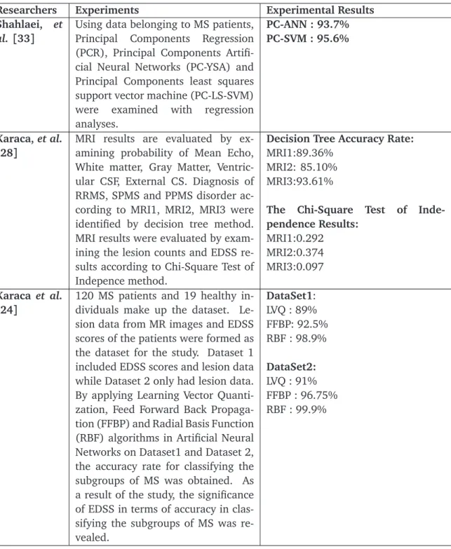
Researchers Experiments Experimental Results Shahlaei, et

al. _[33]

Using data belonging to MS patients,

Principal Components Regression

(PCR), Principal Components Artifi-cial Neural Networks (PC-YSA) and Principal Components least squares support vector machine (PC-LS-SVM)

were examined with regression

analyses.

PC-ANN : 93.7% PC-SVM : 95.6%

Karaca,et al.

[28]

MRI results are evaluated by ex-amining probability of Mean Echo, White matter, Gray Matter, Ventric-ular CSF, External CS. Diagnosis of RRMS, SPMS and PPMS disorder ac-cording to MRI1, MRI2, MRI3 were identified by decision tree method. MRI results were evaluated by exam-ining the lesion counts and EDSS re-sults according to Chi-Square Test of Indepence method.

Decision Tree Accuracy Rate:

MRI1:89.36% MRI2: 85.10% MRI3:93.61%

The Chi-Square Test of Inde-pendence Results:

MRI1:0.292 MRI2:0.374 MRI3:0.097

Karaca et al.

[24]

120 MS patients and 19 healthy in-dividuals make up the dataset. Le-sion data from MR images and EDSS scores of the patients were formed as the dataset for the study. Dataset 1 included EDSS scores and lesion data while Dataset 2 only had lesion data. By applying Learning Vector Quanti-zation, Feed Forward Back Propaga-tion (FFBP) and Radial Basis FuncPropaga-tion (RBF) algorithms in Artificial Neural Networks on Dataset1 and Dataset 2, the accuracy rate for classifying the subgroups of MS was obtained. As a result of the study, the significance of EDSS in terms of accuracy in clas-sifying the subgroups of MS was re-vealed.

DataSet1: LVQ : 89% FFBP: 92.5% RBF : 98.9%

DataSet2:

2. Material and Methods

2.1. Patient Details

In this study, monitored by Hacettepe University Faculty of Medicine, Departments of Neu-rology and Radiology and Primary MR Image center, 120 patients with a definite MS diagnosis based on the McDonald criteria with RRMS, SPMS or PPMS were enrolled. All patients were between the ages of 20 and 55.

Level of disability in patients was determined by using the Extended Disability Status Scale (EDSS). MRI is obtained with a 1.5 Tesla device (Magnetom, Siemens Medical Systems, Er-langen, Germany). Lesions on T2-weighted turbo spin-echo (TSE) sequences were counted in metric units. The brain stem, corpus callosum-periventricular region, including the upper cer-vical lesions in the three regions were included in the information. Magnetic resonance read for three regions lesion in the years to the information changes (number of increments/reductions in size) were compared based on the EDSS scores of years and changes within the clinical di-agnostics were compared with MS. While observing the duration of the disease, there were minimum three years between the first and second MRI scans and there were maximum 8 or 10 years between the second and third and MRI scans. The outcomes of the MS patients have been identified (associated) through EDSS scores by a neurologist using MRI results

[23, 24, 26, 27].

2.2. Expanded Disability Status Scale

Expanded Disability Scale (EDSS) is partly based on the measurements of eight regions known as functional system in the central nervous system. First, the scale measures the tem-porary numbness in the face or fingers or degrees of impairment such as visual impairment. And then, by using walking distance, it measures the disability in terms of mobility[26].

Functional systems measured with EDSS:

(i) Pyramidal: voluntary movements

(ii) Brain stem: eye movements, senses, face movements, functions like swallowing

(iii) Vision

(iv) Brain: memory, concentration, temperament

(v) Cerebellum: balance and coordination of movements

(vi) Sense

(vii) Bowel and bladder

Table 3: Description of EDSS Scores.[6, 12, 26]

Score Description

1.0 No disability, minimal signs in one FS

1.5 No disability, minimal signs in more than one FS

2.0 Minimal disability in one FS

2.5 Mild disability in one FS or minimal disability in two FS

3.0 Moderate disability in one FS, or mild disability in three or four FS. No

impairment to walking

3.5 Moderate disability in one FS and more than minimal disability several

oth-ers. No impairment to walking

4.0 Significant disability but self-sufficient and up and about some 12 hours a

day. Able to walk without aid or rest for 500m

4.5 Significant disability but up and about much of the day, able to work a full

day, may otherwise have some limitation of full activity or require minimal assistance. Able to walk without aid or rest for 300m

5.0 Disability severe enough to impair full daily activities and ability to work

a full day without special provisions. Able to walk without aid or rest for 200m

5.5 Disability severe enough to preclude full daily activities. Able to walk

with-out aid or rest for 100m

6.0 Requires a walking aid - cane, crutch, etc - to walk about 100m with or

without resting

6.5 Requires two walking aids - pair of canes, crutches, etc - to walk about 20m

without resting

7.0 Unable to walk beyond approximately 5m even with aid. Essentially

re-stricted to wheelchair; though wheels self in standard wheelchair and trans-fers alone. Up and about in wheelchair some 12 hours a day

7.5 Unable to take more than a few steps. Restricted to wheelchair and may

need aid in transferring. Can wheel self but cannot carry on in standard wheelchair for a full day and may require a motorized wheelchair

8.0 Essentially restricted to bed or chair or pushed in wheelchair. May be out

of bed itself much of the day. Retains many self-care functions. Generally has effective use of arms

8.5 Essentially restricted to bed much of day. Has some effective use of arms

retains some self-care functions

9.0 Confined to bed. Can still communicate and eat.

9.5 Confined to bed and totally dependent. Unable to communicate or

eat/swallow

10.0 Death due to MS[12, 26]

degrees can be 0 for normal condition and may rise up to 5 or 6 for conditions where the impairment is highest. By adding the movement and daily life limitations to these functional system degrees, we defined the 20 steps of EDSS[21]. The EDSS quantifies disability in eight Functional Systems (FS) and allows neurologists to assign a Functional System Score (FSS) in each of these data are applied by Tanagra software[12, 26].

2.3. Magnetic Resonance Imaging (MRI)

MR scanner utilizes strong magnetic fields to yield the view of the brain and spinal cord. An MR image can reveal inflammatory or damaged tissue regions in the central nervous system

[16, 22]. Figure 1a presents an MR image of a healthy individual while Figure 1b shows the

MR image of an MS patient[23, 26]. Lesion numbers in the MR image of patients taken by a

radiologist at regular intervals have been used for the study.

(a) Healthy Patient[23, 26] (b) MS Patient[23, 26]

Figure 1: MR Images of Patient’s Brains

In this study, we used the number of lesions according to the locations of the brain, and EDSS score for modeling in Table 4.

Table 4: Feature Extracted from MR Images and Representation of Classes and EDSS.

Feature Explanation Explanation

EDSS ranges between 1 and 10

RRMS Integer Number (0)

PPMS Integer Number (-1)

SPMS Integer Number (1)

Lesions the number of lesion diameter that has formed in three

different parts of the brain

has 3 classes (RRMS, PPMS, SPMS), and the data has been applied on Radial Basis Function, Polynomial, Sigmoid and Linear kernels.

Table 5: Training Set Matrix Dimensions

Vector Size Training Set 1 120x227

Training Set 2 120x228

2.4. Support Vector Machines

SVM is a modern classifier which is able to make very good generalizations structuring linear classification boundaries in multidimensional space through kernel[5, 9, 25, 30, 31, 36]. In this study, the subgroups of the disorder, namely RRMS, SPMS, and PPMS as well as classifier performance estimations for MS subgroups has been obtained on different kernels, using the

LIBSVM implementation of the SVM algorithm [7]. SVM design is split by hyperplane [31]

which represents the decision limits; the observations which define the boundaries are called "support vectors". Class estimation is made based on these decision limits. In SVM, a maximum level of accuracy is achieved in the estimation of class prediction of a new set of data formed through the use of optimum decision limit from training data. When class representation belonging to the data is not divided in linear fashion, the formation of decision limit on extreme plane between the classes is an optimization problem. For the solution of such a problem, it is necessary to identify the function between two points as(x,f(x))using the variables in the data set, as seen here:

f₀(x) (1)

f_i(x)≤0,i=1, . . . ,m (2)

h_i(x) =0,i=1, . . . ,p (3)

If the classes cannot be classified in a linear fashion, the optimization problem in SVM is placed to the new space through non-linear based functions. The length of the new space is bigger than that of the initial space[13]. The complexity of it is done through a learning method that is not related to the number of dimension. While finding the best hyperplane, complexity in the optimization problem is written based on the sample number (120). In this way, cross checking has been done while transferring from base functions to the kernel functions. The point that is the least based onw₀values or the biggest point based onaT ≥0 values is found

[13](αandwwill be defined shortly). xεR

n

represents optimization variable, f₀ :Rn →Ris the cost function. It represents the constant functions that are not equal. h_i :Rn →R represents the cost function that is equal

[29].

xεRnmeans variable, D means domain,p∗means optimum value[15]. Lagrangian;

L:Rn×Rm×Rp→R, withd omL=D xRm×Rp, (5)

With Lagrangian Dual Function the lowest level p∗is found.

g:Rm×Rp→R (6)

g(λ,ν) =inf

xεDL(x,λ,ν) (7)

=inf

x∈D f0 x

+

m X

i

λifi x

p X

i

νihi x

(8)

minw,b,ξ

1 2w

T_w+c l X

i=1

ξi (9)

φ(xi),xi represents the data set in Training Set 1 and Training Set 2. For Training Set 1x

is 120×227, and for Training Set 2 x is 120×228 sized matrix. c parameter represents our

classes, and these are RRMS, SPMS and PPMS.wsolves the dual problem in the data set with

3 classes through the equation 10 given below.

After having reached the solution with equation for the dual problem[25, 26], the optimum value is found forw,

w=

l X

i=1

y_iαiφ(xi) (10)

through[13].

s g n(wTφ(x) +c) =s g n(

l X

i=1

y_iαiK(xi,x) +c) (11)

the class determination of MS subgroups, the decision is given based on the function[7, 13]. Based on parameters, with Grid Search, direct learning is not done for class definers. The best defining performance is done based on cross-validation for this. The frequently used parameter for this is regularizer parameter. The performance evaluation for this study has been performed through multi-class[9].

A second important point in SVM is that the kernel use named as kernel trick in training data samples is in implicit nonlinear form. For instance, the form of data with its dot product taken (inner product) like the ones given in Figure 2 represents the kernel trick. In this way, it is possible to work by passing into different spaces in the data by setting up a linear model (right pane) instead of using nonlinear models (left pane). Data should be split initially by a simple hyperplane to be able to pass into different spaces. C-SVC algorithm was used, which is able to classify SVM data with multiple classes.

Kernel trick acts like a bridge from making transfer from linearity to non-linearity. In reality, it makes the big sized and non-linear input data like a linear algorithm. If the problem is not linear, learning can be done like a linear model by going to a new space through non-linear

base functions. The linear model in the new space corresponds to the non-linear model in the initial space. This approach is used for classification[3, 11, 32, 34].

Figure 2: Demonstrating the Kernel Trick, from a Nonlinear Model in the Original Data Space (left pane) to a Linear Model in the Feature Space (right pane), via the implicit mapφ.[30]

L_p=1/2kwk2−

N X

t=1

αtrt wTxt+w₀)−1] (12)

Lp=1/2kwk2− N X

t=1

αtrt wTxt+w0) +

N X

t=1

αt] (13)

Through equation 13, Lagrange terms are added. Derivative is taken based on the parameters and reset to zero.

∂L_p/∂w=0⇒w=

N X

t=1

αtrtxt (14)

∂L_p/∂w=0⇒

N X

t=1

αtrt =0 (15)

In this case, the conjugate,

Ld=1/2(wTw)−wt X

t

αtrtxt−w0

X

t

αtrt+X

t

αt

=−1/2(wtw) +X

t

αt

=−1/2X

t X

s

αtαsrtrs(xt)Txs+X

t

αt,

(16)

[11, 20, 32, 34]. If there is a kernel function, there is no need to conjugate to the new space. In reality, there is a kernel function that corresponds to for each valid kernel but it is easier than using K(xt,x) [11, 20, 32, 34]. φ(xt)or φ(x)values. In recent years, it has become a more common practice to keep the data sets in K kernels instead ofφ(x). It is particular easier for keeping theN×N matrix[3, 11, 20, 32, 34].

C-SVC represents two classes or multiple classes. C represents the number of classes. This study C has three classes which are, RRMS, SPMS and PPMS.

Accuracy rate estimation has been made by getting a class achievement as a result of apply-ing the Radial Basis Function, Polynomial, Sigmoid, Linear, respectively. C-SVC kernel has been applied separately onto the dataset split by hyper plane, and the class achievement has been measured based on 10-fold cross validation. The two class training set is, XiεRn,I =1, . . . ,l

class labels are y_iε[−1, 1][10, 30, 31].

The classification optimization of C-SVC algorithm is; constraints are:

y₁ wTΦ x₁+b≥1−ξi,ξi ≥0,i=1 . . .l (17)

Definition of dual problem is as follows:

minα

1 2α

T_Qα−eT_{, 0≤α}

i ≤C,i=1 . . .l (18)

With constraints yTα =0, where eis a vector of all ones C >0 is upper bound, Q is a l×l positive semi define matrixQ_{i j}= y_iy_jK(x_t,x)andK(x_t,x) =φ(xT_t)φ(xj))is called the

kernel functionφtransforms training vectorsx_tinto a higher dimensional space. In this study, there are two different data sets.

Decision function is;

sgn(

l X

i=1

yiαiK(xt,x) +c) (19)

K(x_t,x) =e x p(−γkx_t−xk2),γ >0 (20)

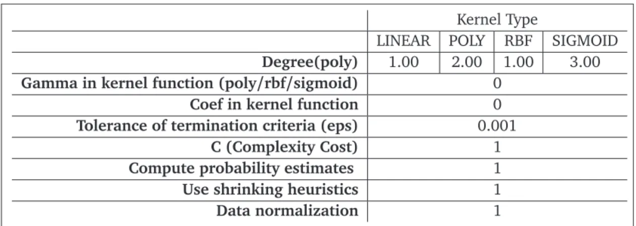
optimization problem has arisen since the data set has multiple classes. It has been possible to overcome this situation by doing experimental applications on different kernel types. The optimized values of the parameters in the data set have been presented in Table 6. As a result of our experimental studies, the best classifying estimation in SVM has been yielded through Linear, RBF, Polynomial and Sigmoid Kernel on account of the nature of our data set. For this reason, these four main kernel types have been preferred[15].

Table 6: C-SVC Kernel Parameters

Kernel Type

LINEAR POLY RBF SIGMOID

Degree(poly) 1.00 2.00 1.00 3.00

Gamma in kernel function (poly/rbf/sigmoid) 0

Coef in kernel function 0

Tolerance of termination criteria (eps) 0.001

C (Complexity Cost) 1

Compute probability estimates 1

Use shrinking heuristics 1

Data normalization 1

As to (Radial Basis Function) Kernel, in the study Gaussian kernel type has been used.

Sigma (s) plays a major role in the performance of the kernel. svalue should be tuned with

keen attention based on the available problem. If an extreme value is assigned for the sigma, the exponential value acts almost linearly and loses power for the big sized non-linear data

[11, 15, 20]. Thus, there will be deprivation of function regulation, and the determination threshold will be sensitive for noise. Gaussian kernel has been chosen for the MS data set that is not classified linearly. For this reason, it has been deemed to be the appropriate kernel in our data set. svalue is chosen to be 3.

The equation,

K xt,x=e x p − k x

t_{−x k}2 2s2

, (21)

represents the global kernel. xt determines the center and sdetermines the radius that has

been formerly made constant. When the radius is large, hyperplane becomes more flat. The best results are found through cross validation. While adjusting the two upper parameters with cross validation, searching is done in two dimensions for all (c and s2) possible value duals.

Polynomial kernel is a kernel that is appropriate for the non-stationary data set. Like the data set used in our study, it is the appropriate kernel type for the normalized training data set[30]. For degreeq,

K(xt,x) = (xTxt+1)q, (22)

kernel,qdegree is chosen as 2; forq=2:

K(x,y) =(xTy+1)2

=(x₁y1+x2y2+1)2

=1+2x₁y₁+2x₂y₂+2x₁y₁x₂y₂+x2₁y₁2+x₂2y₂2

. (23)

The kernel,

φ x= 1,p2x1,

p

2x2,

p

2x1x2,x12,x 2 2

T

(24)

corresponds to the inner product of the base function.

Sigmoid Kernel is known as the Multi-layered Perceptron kernel [20]. It is used as the activation function in artificial neurons. This kernel has been preferred since the MS data set is appropriate for multi-layer learning. In addition to this, it yields a good level of performance in practice although it is conditionally positive definite[3, 29]. Alpha value gets 1/N value,

whereN is the number observations. For both our training and testing sets,N=120.

K(xt,x) =tanh(γ〈xt,x〉+c) (25)

K(xt,x) =tanh(〈x〉+c) (26)

ranges between -1 and+1.

Linear Kernel is the most simple kernel, and 〈x,y〉 is given in the input. c has constant value. It is used generally in kernel algorithms[15].

K(xt,x) =〈xt,x〉+c (27)

K(xt,x) =x+c (28)

The main purpose of our study is to be able to define the subgroups of MS, namely RRMS, SPMS and PPMS through SVM algorithm. At the same time, the purpose is to show the ac-curacy of using multi kernel use in defining MS subgroups. SVM algorithm makes the class estimation of the data with classes more than two with higher accuracy. In this respect, this study is the first of its kind in literature since it has conducted the performance evaluation of C-SVC algorithm kernel types for the classification of MS subgroups on MS data set.

3. Results

MR images and EDSS scores of have been utilized in our study while carrying out the di-agnosis. MRI results are evaluated by examining the lesion counts and EDSS scores. LibSVM, multiclass library of SVM supervised algorithm which is one of the popular machine learning algorithms has been used for the diagnosis of the disorder regarding RRMS, SPMS and PPMS. The study has been conducted on two different data sets.In the first data set, EDSS score has been removed from the data set to emphasize the significance of the parameter. For this rea-son, it is a matrix of size 120×227. The second data set is a matrix of size 120×228 with EDSS scores and MRI data of 120 patients (the number of lesion diameter/width for three different regions separately). The evaluation has been made by applying Radial Basis Function, Poly-nomial, Sigmoid and Linear kernel on two different datasets for multiclass SVM (C-Support Vector Classification)[10]. By using C-SVC[5, 25, 36]algorithm used for applications which SVM algorithm exceeds two classes, the performance classification analysis of MS subgroups (RRMS, SPMS, PPMS) has been performed. LibSVM library has been used for this purpose.

The verification has been made by 10-fold cross validation which is one method used in statistics. In addition to this, during the classification stage of C-SVC kernel methods (RBF ker-nel, Polynomial kerker-nel, Sigmoid kerker-nel, Linear kernel), computation time has been provided in a comparative fashion. Accuracy of the data has been validated and applied onto C-SVC algorithm kernel types separately. In addition, the verification of the accuracy rates has been made by 10-fold cross validation, which is one of the relevant statistical methods. In the end, while forming the classification of kernel types, the time elapsed and test achievement results have been compared with each other.

The results of our study have been obtained using Tanagra software, which is one of the data mining tools†. LibSVM library has been used for this purpose.

Table 7: Classification Achievement Rates and Classification Computation Time Based on Ker-nel Types for Training Set 1.

Kernel Type Classification Rate Computation Time (ms)

Radial Basis Function 99.658% 1217

Polynomial 99.633% 1154

Sigmoid 99.615% 1202

Linear 99.741% 858

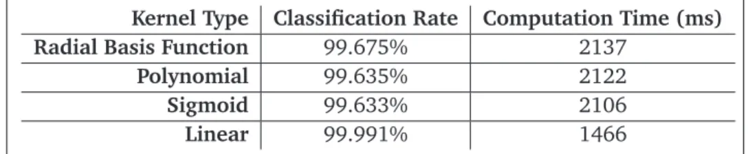
Table 8: Classification Achievement Rates and Classification Computation Time Based on Ker-nel Types for Training Set 2.

Kernel Type Classification Rate Computation Time (ms)

Radial Basis Function 99.675% 2137

Polynomial 99.635% 2122

Sigmoid 99.633% 2106

Linear 99.991% 1466

Based on analyses in Table 7, while forming the classification model belonging to kernel

types applied onto the 120×227 data set, working time elapsed and test achievement rate

have been evaluated. The least classification duration belongs to the Linear kernel. When classification achievement rate is analyzed, the best performances are seen in Linear, RBF, Polynomial and Sigmoid kernel, respectively.

The Radial Basis Function (RBF) kernel has the highest duration of working time in the

classification regarding 120×228 data set given in Table 8. On the other hand, the lowest

working time belongs to Linear kernel. When the performance result in classification is ex-amined, the most successful kernel is Linear kernel, followed by RBF, Polynomial kernel, and Sigmoid kernel, respectively.

4. Conclusions

The aim of this study is to be able to carry out a classification using C-SVC algorithm of SVM algorithm from the data set regarding the lesion counts in the lesion diameters obtained from the MR images of people with RRMS, SPMS and PPMS subgroups of MS. In addition, EDSS scores of each patient have been used. Based on the four different kernel types of C-SVC algorithm (Radial Basis Function, Polynomial, Sigmoid and Linear kernel) classification has been made.

Classification has been made based on the four different kernel types of C-SVC algorithm (Radial Basis Function, Polynomial, Sigmoid and Linear kernels). The number of lesion diame-ter taken from the MR images and EDSS scores of the MS patients make up the dataset. C-SVC algorithm has been applied onto kernel types separately, the achievements thereof have been verified and compared based on 10-fold cross validation, which is one of the relevant statistical methods.

classification and the performance in classification are examined in both of the datasets. The reason for this is theγandrparameters in Sigmoid kernel. Linear kernel type has been formed by adding the EDSS parameter into the most accurate kernel type dataset.

This study highlights the fact that it is possible to use C-SVC algorithm while doing clas-sifications in static and non-static medical data. It has also been aimed that the study could provide a reference in the view that achievement rate can be received based on different kernel types. The findings the study have yielded, like the data such as lesion diameter, number etc. received from the MR images of the patients, EDSS and doctors’ guidance were also elements that have been made use of.

ACKNOWLEDGEMENTS The authors would like to express their gratitude to Hacettepe Uni-versity Medical Faculty, Neurology and Radiology Department in Primer Magnetic Resonance Imaging Center, and to radiologists Eray Atlı MD and Mehmet Yorubulut MD, for their collab-oration with domain knowledge and manual segmentation of the input dataset.

References

[1] H. Alashwal, S. Deris, and R.M. Othman. A bayesian kernel for the prediction of protein-protein interactions.World Academy of Science, Engineering and Technology, 51:928–933, 2009.

[2] Alisneaky. Support vector machine — Wikipedia, the free encyclopedia, 2011. [Online; accessed 17-April-2011].

[3] E. Alpaydın. Yapay Ö˘grenme. Bo˘gaziçi Üniversitesi Yayınevi, Istanbul, Turkey, 2013.

[4] J. Basak. A least square kernel machine with box constraints. In 19th International

Conference on Pattern Recognition, pages 1–4, Florida, USA, 2008. IEEE.

[5] K. Bendfeldt, S. Klöppel, T.E. Nichols, R. Smieskova, P. Kuster, S. Traud, N.M. Lenke, Y. Naegelin, L. Kappos, E.W. Radue, and S.J. Borgwardt. Multivariate pattern

classifi-cation of gray matter pathology in multiple sclerosis. NeuroImage, 60(1):400–408, Mar

2012.

[6] R. Bergamaschi, S. Quaglini, M. Trojano, M.P. Amato, E. Tavazzi, D. Paolicelli, V. Zipoli, A. Romani, A. Fuiani, E. Portaccio, C. Berzuini, C. Montomoli, S. Bastianello, and V. Cosi. Early prediction of the long term evolution of multiple sclerosis: the bayesian risk esti-mate for multiple sclerosis (BREMS) score. Journal of Neurology, Neurosurgery & Psychi-atry, 78(7):757–759, Dec 2006.

[7] B.E. Boser, I.M. Guyon, and V.N. Vapnik. A training algorithm for optimal margin

clas-sifiers. In Proceedings of the Fifth Annual Workshop on Computational Learning Theory,

[8] S. Boughorbel, J. Tarel, and N. Boujema. Generalized histogram intersection kernel for image recognition. InIEEE International Conference on Image Processing, volume 3, pages III–161, Genoa, Italy, 2005. IEEE.

[9] C.C. Chang and C.J. Lin. LIBSVM: A library for support vector machines. ACM

Transac-tions on Intelligent Systems and Technology, 2:27:1–27:27, 2011.

[10] C. Cortes and V. Vapnik. Support-vector networks. Machine Learning, 20(3):273–29,

1995.

[11] S. Fomel. Inverse b-spline interpolation, 2000.

[12] M. Gaspari, G. Roveda, C. Scandellari, and S. Stecchi. An expert system for the evaluation of EDSS in multiple sclerosis.Artificial Intelligence in Medicine, 25(2):187–210, Jun 2002.

[13] M.G. Genton. Classes of kernels for machine learning: a statistics perspective. The

Journal of Machine Learning Research, 2:299–312, 2002.

[14] H. Gutermana, Y. Nehmadi, A. Chistyakov, J.F. Soustiel, and M. Feinsod. A comparison

of neural network and bayes recognition approaches in the evaluation of the brainstem trigeminal evoked potentials in multiple sclerosis. International Journal of Bio-Medical Computing, 43(3):203–213, Dec 1996.

[15] B. Hamers. Kernel models for large scale applications. PhD thesis, Katholieke Universiteit Leuven, 2004.

[16] C.H. Hawkes and G. Giovannoni. The McDonald criteria for multiple sclerosis: time for clarification. Multiple Sclerosis Journal, 16(5):566–575, Mar 2010.

[17] C. Hirst, G. Ingram, R. Swingler, D.A.S. Compston, T. Pickersgill, and N.P. Robertson. Change in disability in patients with multiple sclerosis: a 20-year prospective population-based analysis.Journal of Neurology, Neurosurgery & Psychiatry, 79(10):1137–1143, Oct 2008.

[18] T. Hofmann, B. Schölkopf, and A.J. Smola. Kernel methods in machine learning. The

annals of statistics, 36(3):1171–1220, 2008.

[19] T. Howley and M.G. Madden. The genetic kernel support vector machine: Description

and evaluation. Artificial Intelligence Review, 24(3-4):379–395, 2005.

[20] C-W Hsu and C-J Lin. A comparison of methods for multiclass support vector machines.

IEEE Transactions on Neural Networks, 13(2):415–425, Mar 2002.

[21] R. Karabudak. MS ile Ya¸samak. A¸sina Kitaplar, Turkey, 2006.

[23] Y. Karaca. Constituting an Optimum Mathematical Model for the Diagnosis of Multiple Sclerosis. PhD thesis, Marmara University, 2012.

[24] Y. Karaca and ¸S. Hayta. The significance of artificial neural networks algorithms clas-sification in the multiple sclerosis and its subgroups. International Advanced Research Journal in Science, Engineering and Technology (IARJSET), 2(12):1–7, Dec 2015.

[25] Y. Karaca, ¸S. Hayta, and R. Karabudak. The application of support vector machines for the classification of multiple sclerosis subgroups. InThe International Conference Mathe-matical and Computational Modelling in Science and Technology, Abstract Book, page 95, Izmir University, Izmir, 2015.

[26] Y. Karaca, O. Osman, and R. Karabudak. Linear modeling of multiple sclerosis and its

subgroubs.Journal of Clinical Research of Pediatric Endocrinology, 21(1):7–12, Mar 2015.

[27] Y. Karaca and G. Sayıcı. Bayesian networks for subgroups of multiple sclerosis.

In-ternational Journal of Electronics, Mechanical and Mechatronics Engineering (IJEMME), 3(1):455–462, 2013.

[28] Y. Karaca, G. Sayıcı, and R. Karabudak. Application of decision tree for classification of multiple sclerosis diagnosis, expanded disability status scale and lesion numbers. In 7th International Image Processing & Wavelet on real World applications conference (IWW2013), pages 115–129, Valencia, 2013.

[29] C.A. Micchelli. Interpolation of scattered data: distance matrices and conditionally pos-itive definite functions. Constructive approximation, 2(1):11–22, 1986.

[30] J. Novakovic and A. Veljovic. C-support vector classification: Selection of kernel and

parameters in medical diagnosis. In IEEE 9th International Symposium on Intelligent

Systems and Informatics, pages 465–470, Subotica, Serbia, Sep 2011. IEEE.

[31] F. Parzlivand and A. Shahrezaee. Radial basis functions for the solution of an inverse

problem of mixed parabolic-hyperbolic type.European Journal of Pure and Applied

Math-ematics, 8(2):239–254, 2015.

[32] H. Sahbi and F. Fleuret. Kernel methods and scale invariance using the triangular ker-nel. Technical Report RR-5143, French Institute for Research in Computer Science and Automation, 2004.

[33] M. Shahlaei, A. Fassihi, and L. Saghaie. Application of PC-ANN and PC-LS-SVM in QSAR

of CCR1 antagonist compounds: A comparative study. European Journal of Medicinal

Chemistry, 45(4):1572–1582, Apr 2010.

[34] A. Vedaldi and Andrew A. Zisserman. Efficient additive kernels via explicit feature maps. IEEE Transactions on Pattern Analysis and Machine Intelligence, 34(3):480–492, 2012.

[35] L. Zhang, W. Zhou, and L. Jiao. Wavelet support vector machine. IEEE Transactions on

[36] C.Y. Zhao, R.S. Zhang, H.X. Liu, C.X. Xue, S.G. Zhao, X.F. Zhou, M.C. Liu, and B.T. Fan. Di-agnosing anorexia based on partial least squares, back propagation neural network, and

support vector machines. Journal of Chemical Information and Modeling, 44(6):2040–