Constant Time Queries for Energy Efficient Paths in Multi-hop Wireless Networks

Constant Time Queries for

Energy Ef

fi

cient Paths in

Multi-hop Wireless Networks

Stefan Funke

_{, Domagoj Matijevi´c}

_{and Peter Sanders}

2_{Universit¨at Karlsruhe, Fakult¨at f¨ur Informatik, Karlsruhe, Germany}

We investigate algorithms for computing energy efficient paths in ad-hoc radio networks. We demonstrate how advanced data structures from computational geometry can be employed to preprocess the position of radio stations in such a way that approximately energy optimal paths can be retrieved in constant time, i.e., independent of the network size. We put particular emphasis on actual implementations which demonstrate that large constant factors hidden in the theoretical analysis are not a big problem in practice.

Keywords: ad-hoc and sensor networks, routing, power control, wireless LANs, computational geometry.

1. Introduction

Ad hoc radio networks are an attractive way to quickly build a communication infrastructure without slow and expensive deployment of a cable backbone. Since many of the stations will be battery or solar powered, energy consump-tion becomes a major issue in such networks. We use the following widespread model for en-ergy consumption: The stations are defined by a set of npoints in the plane. The energy con-sumption for communication between pointsp

and q is assumed to be ω(p,q) = |pq|σ for some constant σ > 1, where |pq| denotes the Euclidean distance between p and q. In free space σ = 2 gives an exact physical model. Values σ ∈ (2,4)can be used to approximate absorption effects[18, 16].

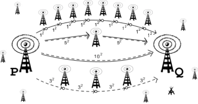
We are now looking for paths connecting arbi-trary pairs of points that minimize energy con-sumption subject to the additional constraint that at mostkhops are used(see Figure 1).

Figure 1.A Radio Network example with 9,4,2,1-hop paths fromPtoQwith costs 9, 36, 50, 100.

Limiting the number of hops accounts for dis-tance independent energy consumption (e.g., for encoding and decoding signals) as well as for reliability and latency problems connected with paths that use an unbounded number of hops. For refinements of the model refer to Section 4. In our considerations we assume k

to be a rather small constant.

This problem can be solved optimally in time

O(kn2)using well known algorithms for com-puting shortest paths, as we will see in Section 2. However, this would be much too slow for all but very small networks. In[11]we therefore devel-oped an algorithm that produces paths that are within a factor(1+)from optimal inconstant timeindependent of the size of the network. If

kandare considered constants, the algorithm needs preprocessing timeO(nlogn)and space

factors and it uses sophisticated data structures from computational geometry for which there is little experience with respect to their practi-cality.

The purpose of this paper is to help close this gap between theory and practice. We study a num-ber of implementations of simple algorithms and new heuristics as well as a variant of the approximation scheme from[11], but tuned for more practicability. The solutions we present can be modified to provide for additional re-quirements, like dynamic maintenance or fault-tolerance, which both improve the quality of service₍QoS₎.

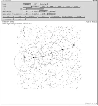
Figure 2.Screenshot of our simulation program.

Related Work

In 1998, Bambos[3]reviewed developments in power control for wireless networks and em-phasized the need for minimum-power routing

protocols. Since then a vast amount of research has been conducted on the issue of energy-conservation in ad-hoc and sensor networks, see for example[13],[16],[17].

In the computational geometry community,Chan, Efrat, and Har-Peled [10, 9] have made sev-eral interesting observations for energy opti-mal paths with unbounded number of hops. They observe that it suffices to compute shortest

paths in the Delaunay triangulation of the input points, i.e., optimal paths can be computed in timeO(nlogn). Note that this approach com-pletely collapses for khop paths because most Delaunay edges are very short. They also give a sophisticated O(n4/3+γ_{) time algorithm for}

arbitrary monotone cost functions ω(p,q) = f_(|pq_|), where γ is any positive constant. For quadratic cost functions with offsetsω(p,q) = |pq|2_{+C, Beier, Sanders, and Sivadasan reduce}

that toO(n1+γ_{), toO(knlogn)fork-hop paths,}

and toO(logn)time queries fortwo hoppaths using linear space and O(nlogn) time prepro-cessing. The latter result is very simple, it uses Voronoi diagrams and associated point location data structure.

2. Exact Algorithms for Finding Energy-minimizing k-hop Paths

Before we get to the actual algorithms let us give a more formal and abstract definition of our energy-minimizingk-hop path problem: Given a setPofnpoints inZ2and some constant

k, report for a given query pair of pointss_,t_∈P, a polygonal path π = π(s,t) = v0v1v2. . .vl,

with vertices vi ∈ P andv0 = s,vl = t which

consists of at mostksegments, i.e. l ≤k, such that its weightω(π) =0≤i<lω(vi,vi+1)is

minimized. Byπopt = πopt(s,t)we denote the

optimal path fromstotunder this criterion. In the following we assume that the weight func-tion ω is of the form ω(p_,q_{) = |}pq_|σ with

σ >1(the caseσ ≤1 is trivial as we just need to connect s and t directly by one hop). For more general weight functions, in particular if we also have a constant, node-dependent offset likeω(p,q) = |pq|σ +cp, we refer to Section

4 for possible refinements of the algorithms we present in this paper.

2.1. The Naive Approach

The point set Ptogether with the weight func-tion ω induces the complete weighted graph

G(P,E,ω)with vertex setPand edges(v,w)∈ E of weightω(v,w), ∀v = w ∈ P. This graph hasn₍n₋1_)/2 edges and for a given query pair

s,t ∈ P we are looking for the shortest path

πopt =π(s,t)optfromstotinGwhich uses no

This path πopt can be easily computed by

dy-namic programming. Let π(s,v)(opti) denote the

shortest path from the source node s to node

v which uses no more than i edges. Clearly

π(s,v)(opt1) = sv, ∀v ∈ P − {s}. π(s,v)(opti) is

determined asπ(s,w)opt(i−1)vwithwchosen such

thatω(π(s,w)opt(i−1)) +ω(w,v)is minimized.

The naive dynamic programming approach fills a table of dimensionn×kusing the above rules:

• ∀v_∈P: π(s_,v₎(_opt1) _←sv • fori=2 tokdo∀v∈P:

∗ computeπ(s_,v₎(_opti) by looking at all possiblew, the concatenations

π(s,w)(opti−1)vand their weights

ω(π(s,w)opt(i−1)) +ω(w,v)

Clearly, this algorithm has running timeO(k·n2₎

as we have to fill in a table of sizek_·nand de-termine the value of one cell costs O(n) since we look at all possible w _∈ P. It is not hard to figure out that this approach only works for extremely small problem instances and even for those, it is rather slow as we get a quadratic behavior innper query.

2.2. Neighborhood Pruning

One obvious improvement to the above algo-rithm is due to the observation that if we are in-terested in the energy-minimalk-hop path from

s to t, points which are “far” away from the segment st cannot be of any use for the solu-tion. So, letDdenote the distance between the query points, i.e. D = |st|. If we restrict our dynamic programming approach to all points

p ∈Pwhich have distance at mostλ ·Dto the segment|st|– we call this theλ-neighborhood of st–, what is the smallest value ofλ such that we can still compute the optimal solution? See Figure 3 for an example ofλ-neighborhoods. It is not hard to see that if the optimal path πopt

leaves the region which has distance at most

λ ·D to st, the sum of the Euclidean lengths of the segments of this path must be at least 2·D·λ2_{+1/4. And as the “optimal”}

strat-egy to chop a path of any given length into k

pieces such that the overall energy is minimized

is to chop it into pieces of equal length, we get the following inequality

(2·D·λ2_+1/4)σ

kσ−1 ≤Dσ

which bounds λ in terms of the cost Dσ that is encountered when taking just one direct hop fromstot. So, we get

λmax =

k2σσ−2 −1 2

Therefore, if there are only few points in the neighborhood of the query pointssandt(more precisely, if there are only few points within distanceλmax|st|), we first use a standard range query data structure from computational geom-etry to report all those points and run the naive approach only for those and we can expect a reasonably fast query time, which is now only quadratic in the number of points in the neigh-borhood ofsandt.

Cascaded Neighborhood Pruning

In the neighborhood pruning approach we used the one-hop cost as an upper bound to limit the size of the neighborhood that still needs to be explored. Clearly, if we had a better up-per bound (i.e. tentative solution)for the cost of getting from s to t within k hops, we could restrict the size of the neighborhood even fur-ther. How could such a better tentative solution be obtained? Well, we could start with a very small value forλ, evenλ = 0 is viable, it just restricts the neighborhood to all points which lie on the segmentst. We run our dynamic pro-gramming approach on that set of points and use the outcome to bound the maximal value of λ

that we have to consider to guarantee the opti-mal solution is found. So this cascaded strategy could be implemented as follows:

1. λ ←0.1 2. upper=|st|σ

3. while(2·D·√_kσλ₋2+₁1/4)σ ≤upper

• compute using dynamic program-ming the optimal k-hop path w.r.t. the λ-neighborhood of st, update upper if necessary

The procedure terminates as soon as it can prove that no larger neighborhood has to be inspected, which of course happens no later than after

O(logλmax) rounds. For dense point sets, this will turn out to be a lot more effective than the naive or simple neighborhood pruning strategy without cascading.

s t

λ= 1/11

λ= 5/22

λ= 5/11

Figure 3.λ-neighborhoods of a segmentst.

3. Approximate Algorithms for Finding Energy-minimizing k-hop Paths

The neighborhood pruning approach – though helpful for many problem instances – does not improve the worst-case running time of the dy-namic programming approach as it might be the case that basically all the points are in the neighborhood of the segmentst and have to be inspected.

But if we relax the exactness requirement and only require approximate(1+)solutions, i.e. we are happy with paths π(s,t)app such that ω(π(s_,t₎app) ≤ (1+)·ω(π(s,t)opt) for any > 0 to be chosen from the user, we can do better. In fact, usingGrid Pruningwe can guar-antee a logarithmic query time, whenk, ,σare considered constants.

3.1. Grid Pruning

The idea of Grid Pruning is to place a grid over the neighborhood of the segmentstand first re-port onerepresentativein each of the grid cells (this can be done again using standard geomet-ric range query in timeO(logn)per grid cell). The dynamic programming approach is then only performed on those representative points and the computed path is used as a result of the computation. The smaller, the smaller the

grid-cells, and hence the better approximation of the optimal pathπopt.

In fact, one can show ₍see _[11_]) that putting a grid of cell-width α ·D_/k with α = ₂ln 2√

2σ,

the computed path πapp(s,t) has cost at most (1+)·ω(πopt(s,t)).

The grid pruning algorithm looks as follows: 1. Put a grid of cell-widthα·|st|/kon theλmax

-neighborhood ofstwithα = ln 2 2√2σ.

2. For each grid cellC perform an orthogonal range query to either certify that the cell is empty or report one point inside which will serve as a representative forC.

3. Compute the minimum k-hop path π(s_,t₎

with respect to all representatives and _{s_,t_}

using the dynamic programming approach. 4. Returnπ(s,t).

The gain compared to the previous methods is that we reduce the number of points to be con-sidered toO(σ2·k4σσ−2

2 ), irrespectively how many points there are in the neighborhood ofst. So, consideringk,σ, constants, the query time be-comes O(logn) due to the range queries that have to be performed for each grid cell.

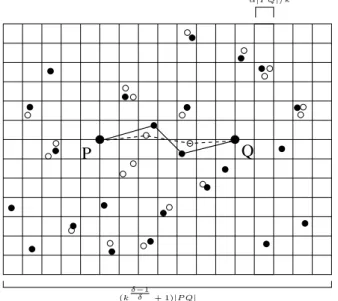
Please look at Figure 4 for a schematic drawing of how the algorithm computes the approximate

k-hop path.

Q P

(kδ−

1

δ + 1)|P Q|

α|P Q|/k

Cascaded Grid Pruning

Clearly, the same trick of looking at small neigh-borhoods ofstfirst, which we have used to im-prove the neighborhood pruning approach, also works here. So first we only put the grid over a very small neighborhood and consider larger and larger neighborhoods until the required ap-proximation guarantee can be proven.

3.2. The Milestone Heuristic

For very dense point sets, there is another very simple heuristic, which uses the observation that in the “ideal” case the segmentstis divided into

ksubsegments of equal length. Clearly, if such ak-hop path can be obtained, it is the optimum path. So, the Milestone Heuristic tries to ap-proximate this “ideal” path by virtually placing the k−1 “ideal” radio stations v1, . . .vk−1 on

st. As these vi are typically not inP, we

per-form for each of them a nearest neighbor query on the point set P and use the outcome as the replacement forvi(each of these queries can be

performed inO(logn)time). Nearest neighbor query data structures from computational ge-ometry are by now standard in many software libraries and very space- and time-efficient im-plementations are available, e.g. in [14]. The algorithm looks as follows:

1. determine “ideal” hop positionsv1, . . . ,vk−1

2. for eachviperform a nearest neighbor query

onPto obtainv_i ∈P

3. outputsv₁. . .v_k−1tas thek-hop path

Unfortunately, this approach can be fooled quite badly if the point setPis not equally distributed and there are large areas without any radio sta-tions in the area betweensandt.

3.3. Path Templates via Clustering

The best query scheme we have seen so far is able to answer a (s,t) query in O(logn) time ₍considering k_,δ, as constants₎. Stan-dard range query data structures were the only precomputed data structures used. Now we are going to explain how additional precomputa-tion can further reduce the query time. More precisely, we are going to show how to precom-pute a linearnumber of k-hop paths, such that

for every (s,t), a slight modification of one of these precomputed path templates is a (1+₎

approximatek-hop path and such a path can be accessed in constant time. Here _{> 0 is the}

error incurred by the use of these precomputed paths and can be chosen arbitrarily small.

3.3.1. The Well-separated Pair Decomposition

First, we will briefly introduce the so-called

well-separated pair decompositiondue to Calla-han and Kosaraju([6]).

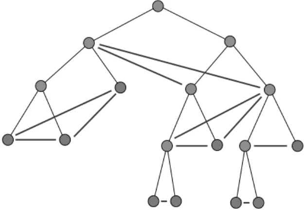
The split-tree of a setP of points in R2 is the tree constructed by the following recursive al-gorithm:

Figure 5.Example of split tree with additional blue edges.

SplitTree₍P₎

1. if size₍P_{) =}1 then return leaf₍P₎

2. partition P into sets P1 and P2 by halving

its minimum enclosing box R(P) along its longest dimension

3. return a node with children(SplitTree(P1),

SplitTree(P2))

We will also use A to denote the node associ-ated with the setAif we know that such a node exists.

For two setsAandBassociated with two nodes of a split tree, d(A,B)denotes the distance be-tween the centers of R(A) and R(B) respec-tively. A and B are said to be well-separated

ifd(A,B)>S·r, whererdenotes the radius of the larger of the two minimum enclosing balls of R₍A₎ andR₍B₎ respectively. S is called the

separation constant. Roughly, this means that the distance between the centers of R(A) and

R(B) is about the same as for any paira ∈ A,

b∈B.

In _[6_], Callahan and Kosaraju present an algo-rithm which, given a split tree of a point setP

with|P|= nand a separation constantS, com-putes in time O₍n₍S2_{+logn))a set of O(n·S}2₎

additional blue edges (A,B) for the split tree, such that

• the point sets associated with the endpoints of the blue edge are well-separated with sep-aration constantS

• for any pair of leaves(a,b), there exists ex-actly one blue edge(A,B)that connects two nodes on the paths fromaandbto their low-est common anclow-estor lca₍a_,b₎ in the split tree

The split tree together with its additional blue edges is called the well-separated pair decom-position W (WSPD).

Minimum enclosing box Minimum enclosing box

Figure 6.ClustersAandBare ‘well-separated’ ifd>s·r.

3.3.2. Application of the WSPD

Intuitively, the W encodes in linear space all

Θ(n2_{) distance relationships in the point set}

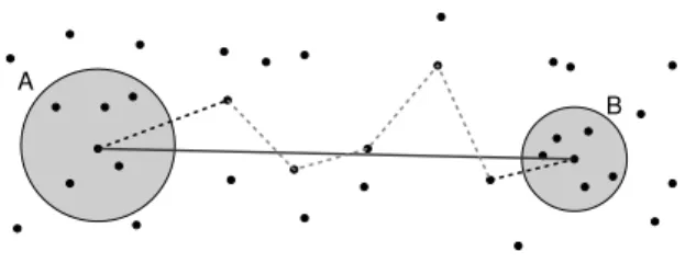
approximately. More precisely, for any query pair (s,t) there exists exactly one cluster pair (A,B)∈W withs∈A,t∈Band|W|=O(n).

So we precompute for each of theseO(n)cluster pairs a good k-hop path between their respec-tive centers (e.g. a(1+)path using the grid pruning strategy), such that at query time, for a given query pair(s,t), it only remains to find the unique cluster pair(A,B)∈ W withs ∈ A,

t ∈B(see Figure 7). We output the associated

k-hop path replacing its first and last nodes with

sandtrespectively.

A

B

Figure 7.Example of the blue-edge connecting well-separated setsAandBand the template path

(red dashed line)saved with it.

Since s _∈ A and t _∈ B and d₍A_,B_{) >} S _·r, the precomputed path between the centers ofcA

andcB is ‘almost’ optimal for the query points

sandt. In fact, one can show formally that the returned path is a(1+_{)approximation of the}

lightestk-hop path fromstot, where_{>0 can}

be chosen arbitrarily by the user(this affects the required choice of the separation constant). See [11]for the details.

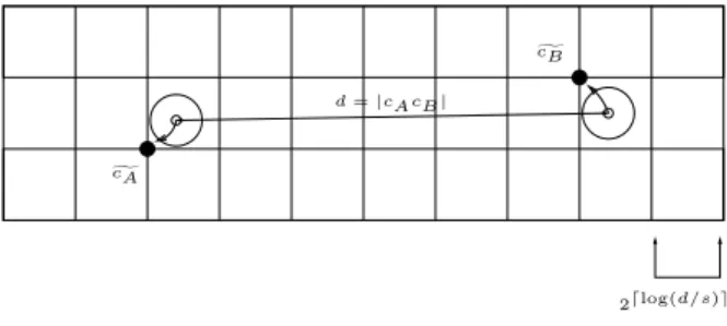
How to retrieve the respective cluster pair(A,B) for a pair of query points(s,t)? The idea of our approach is to round the centerscA,cBof a

clus-ter pair (A,B) ∈ W to canonical grid points

cA,cB and store the associatedk-hop path in a

hash table under the key(cA,cB), see Figure 8.

As grid width we choose the next power of two of dc/s, where dc = |cAcB|. For a query pair

(s,t)we have d = |st| ≈ dc as s ∈ A, t ∈ B

and₍A_,B_)∈W. Hence, the same grid width as used for(cA,cB)can be determined from (s,t)

(up to a factor of 2₎and the path stored under the key ₍cA,cB)can be retrieved. See [11] for

the technical details on this procedure.

In fact, in_[11_]we have shown that for any₍s_,t₎

pair (A,B)of those is good for us. Although it might not be true that s ∈ A, t ∈ B, we know that the cluster centers c_A,c_B are close tosandt(otherwise they would not have been snapped to the same grid points)and therefore the respective k-hop path template is good for us.

g

cA

g

cB

d=|_cAcB|

2log(d/s)

Figure 8.Cluster centerscAandcBare snapped to

closest grid pointscAandcB.

4. Refinements

In the following section we will mention some refinements and extensions that are possible for the presented algorithms, some of which have already found their way into the current imple-mentation.

4.1. Lazy Precomputation

In the path template approach, as presented be-fore, the idea was first to identify a collection of O(n) source-target pairs (namely the cen-ters of the cluscen-ters that are connected by a blue edge in the WSPD)and then precompute a good

k-hop path for each of these pairs. In prac-tice, it will turn out that identifying the blue edges can be done very quickly, and the really time-dominating step is the computation of the template paths₍even when performed using our

O₍logn₎grid pruning approach₎.

But our data structure can easily be modified into a “lazy precomputation” scheme. So at precomputation time, only the blue edges are determined. At query time for a pair(s,t), we first identify the corresponding blue edge. If a template path has been stored for that edge already, we use it (and have spent O(1) time only to answer the query). Only if no template path has been stored already, we compute one

using the grid approach(making this query ex-pensive, i.e. O(logn)). Observe that if a similar query, i.e. a query (s,t) with s near sand t

neart, arrives later, it will find the precomputed template path and can therefore be answered in

O₍1₎.

4.2. Dynamization

All the data-structures that we have used are also – in theory at least – available in a dy-namic version, where updates can be performed in O(logn) time. Hence our whole construc-tion could also be applied for moving and/or changing radio stations. Whether these dy-namic versions of the algorithms are also of practical value, this has to be shown or proven wrong by an experimental study. For more in-formation on dynamic versions of the required data structures, we refer to[2],[1],[7].

4.3. Fault-tolerance

In many real-world applications, reliability and quality of service(QoS)play an important role. In particular, availability of the system has a very high priority. For our application, this means that connections between two sitessandt

should not be prohibited or become very expen-sive if some stations inbetween collapse. There-fore, it is very reasonable to provide for backup paths between the sites, i.e. if one or more sta-tions of an energy efficient path betweensandt

become unavailable, there are other equally ef-ficient paths already precomputed at hand. But this is easy to incorporate into our approach. For each blue edge of the WSPD, instead of

4.4. Startup-costs

In our model as presented, we restrict to a cost model where the required energy to transmit from p to q is ω(p,q) = |pq|σ. However, we can generalize the model with the site depen-dent cost offset Cp > 0, for some site p ∈ S,

in the following manner: the cost of transmit-ting from ptoq is|pq|σ +Cp. The offset cost

Cp accounts for the distance independent

en-ergy consumption of the wireless stations (e.g. the energy consumption of the signal process-ing durprocess-ing sendprocess-ing and receivprocess-ing, or it could be used to steer away traffic from the devices with low battery power).

The good news is that our algorithms in Sec-tion 3 still apply since the offset costCpwill not

influence the size of the λ-neighborhood con-taining the optimal path. However, in the grid pruning approach, one would have to be a little bit more careful and in step 2 of the algorithm report a point with the smallest offset cost(this can be easily incorporated into the standard ge-ometric range query data structures)rather then an arbitrary point inside the cell.

Unfortunately, our Milestone heuristic intro-duced in Section 3.2 in the case of non-negative offset looses its original intuition and it could be easily fooled unless we made some assumption of bound on the offset costs.

5. Implementation

All the algorithms mentioned in the previous sections were implemented using the LEDA li-brary of data structures and algorithms _([14_]). We used the floating-point geometry kernel which represents points in the plane by two

dou-ble coordinates. As range query structure we

employed the LEDA datatype_{point dictionary} which allows range queries in time O(log2)and nearest neighbor queries in O(n) worst-case time. But, as these subroutines never domi-nated the running time in the respective algo-rithms where they were used, we did not put more effort into O(logn)worst-case query time implementations.

A very critical issue was the use of an appropri-ate hashing data structure for accessing the pre-computed template paths. We used the LEDA

type h array which hashes 32-bit integer

val-ues to some information domain. But our im-plementation requires to hash 4-tuples of 32-bit integer values. So we had to reduce the number of bits by a factor of 4. In our experiments the best choice for a hash function was to choose the 3rd to 10th least significant bits of each of these 4 integers and concatenate them to obtain the hash value for the 4-tuple. For other hash functions we tried, the number of collisions in-creased considerably and therefore accesses to the hashing table required going through a long list.

All algorithms were tested within an embedded simulation environment where data can be ei-ther read in or generated and then processed by our algorithms. Using a graphical user-interface, the different parameters and alterna-tive algorithms can be selected and evaluated for running-time and quality of their produced solution. See Figure 2 for a screenshot of our simulation environment.

6. Experiments

We conducted extensive experiments on differ-ent test data and using differdiffer-ent parameters for our algorithms. All running times were mea-sured on a low-end 700 MHz Pentium III with 256 MB of RAM. We used g₊₊2.95.4 with the −O option under a Linux 2.4.19 system.

6.1. Benchmarks

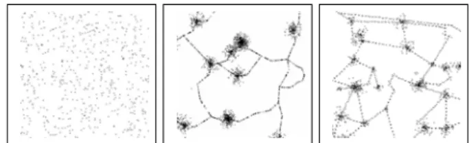
Different test data sets were used to evaluate the quality of our algorithms. See Figure 9 for examples of the generated data.

Figure 9.Examples for test data: random(left), MST-based(middle)and Delaunay-based(right).

6.1.1. Random Data

6.1.2. Simulated Real-world Data

As we had no real-world data available that could be put into a freely-available publication, we simulated the placement of radio stations along a road-network between cities. We had two simple algorithms to generate such data:

MST-based generation We first generated a random set of points₍the cities₎and computed a Euclidean minimum spanning tree. For all the leaves of the tree inside the Convex Hull of the random set we added a new edge. Furthermore, we generated a cluster of points around every city and also put randomly some points along every edge(roads). At the end, we pruned sharp angles.

Delaunay-based generation We first gener-ated a random set of points(the cities)and com-puted the Delaunay triangulation. As we did not want to keep this “triangular” road network, we removed some of the edges under the constraint that the remaining graph was still strongly con-nected to. Then we assigned random weights to the cities and generated radio stations ac-cordingly. Finally, we generated some random stations along the remaining edges.

6.2. Timings and Quality

In the following section we are going to report of the timings and quality of the computed so-lutions for our different test data and varying problem sizes. For the precomputation of the template paths we chose a separation constant of S =5 for the WSPD and = 5 for the grid pruning subroutine. Even though in theory this guarantees only a solution within a factor of 216(!) of the optimal solution, in practice the returned solutions were rather close to the opti-mum. For the used parameters ofk =5,σ =2,

S=5,=5, in fact the returned solutions were not more than 20 % off the optimum on the av-erage. See Tables 1, 2, 3, 4, 5 for the timing and quality results. Note that the ‘WSPD’ column in our tables stands for the "path template" ap-proach from Section 3.3. Furthermore, ‘Brute Force’ and ‘Brute Force pruned’(BF and BFp) columns stand for naive algorithm from Sec-tion 2 with neighborhood pruning and cascaded

neighborhood pruning, respectively. ‘Grid’ col-umn reports results forO₍logn₎approximation algorithm from Section 3.1 while ‘Milestone’ column reports results for Milestone heuristic.

WSPD BF BFp Grid Milestone Av.Time 8.0·10−4 _{0.91 0.24 0.038 0.002}

Max Time 2.0·10−3 _{1.45 1.24 0.080 0.01}

Av.Rel.Err 15% 0 0 2.7% 2.7% Max Rel.Err 49% 0 0 6.5% 20%

σ_rel.err 0.12 0 0 0.018 0.039

Table 1.1000 points randomly generated;k=5,σ=2,

S=5,=5; Query time and quality.

WSPD BF BFp Grid Milest. Av.Time 5.66·10−4 _{14.59 4.75 0.07 0.01}

Max Time 0.003 24.63 14.46 0.099 0.01 Av.Rel.Err 16% 0% 0% 2.6% 0.5% Max Rel.Err 32.6% 0% 0% 4.8% 2.5%

σ_rel.err 0.088 0 0 0.016 0.007

Table 2.4000 points randomly generated;k=5,σ=2,

S=5,=5; Query time and quality.

WSPD BF BFp Grid Milestone Av.Time 1·10−4 _{1.193 0.937 0.009 0.0006}

Max Time 1·10−3 _{1.63 4.03 0.01 0.01}

Av.Rel.Err 14% 0% 0% 3.6% 10.2% Max Rel.Err 38.7% 0% 0% 14.4% 35.9%

σ_rel.err 0.123 0 0 0.047 0.114

Table 3.1000 points from the MST model;k=5,

σ=2,S=5,=5; Query time and quality.

WSPD BF BFp Grid Milestone Av.Time 1·10−4 _{18.6 10.1 0.024 0.011}

Max Time 0.001 27.19 21.09 0.039 0.02 Av.Rel.Err 10.1% 0% 0% 3.3% 14.3% Max Rel.Err 20.5% 0% 0% 8.1% 33.7%

σ_rel.err 0.048 0 0 0.026 0.109

Table 4.4000 points from the MST model;k=5,

WSPD BF BFp Grid Milestone Av.Time 4·10−4 _{0.772 0.303 0.014 5·10}−4

Max Time 0.002 1.13 1.28 0.03 0.01 Av.Rel.Err 17.2% 0% 0% 5.7% 10.7% Max Rel.Err 35% 0% 0% 56% 57%

σ_rel.err 0.101 0 0 0.12 0.134

Table 5.1000 points from the Delaunay model;k=5,

σ=2,S=5,=5; Query time and quality.

From the results you can see that the query time using the WSPD approach remains basi-cally constant, independent of the problem size, which is not true for all other algorithms. In par-ticular, the brute-force variants suffer severely when increasing the problem size, but also the Milestone approach gets slower due to the near-est neighbor queries. The Grid approach also deteriorates a bit, but will saturate at some point (in theory at least₎. With regard to the qual-ity, the brute force approaches are clearly the best since optimal, but also the Milestone ap-proach is not too bad. The results obtained by the WSPD approach are mostly comparable to the Milestone and Grid approaches, but can be tuned by choosing different parameters, as we will see later.

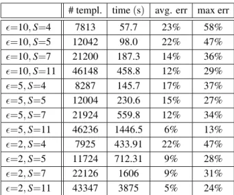
Of course, these very fast query times have their cost, both in terms of time for the precomputa-tion as well as in terms of the space required to store the template paths. For this purpose we look again at the example of 1000 random points, but now vary both(the parameter used for the grid approach when computing the tem-plate paths) as well as S (the separation con-stant for the WSPD). See Table 6 for the results. Apart from the size of the precomputed struc-ture and the preprocessing time, we show the average and maximal relative error that was in-curred by the precomputed paths for 30 random

k-hop queries.

Clearly, the more time and space one is willing to invest into computing good path templates, the better results one gets for the queries. We emphasize that all the precomputation can be done in a lazy fashion as explained in Section 4, so the precomputation time would only con-sist of the time required to construct the WSPD, which is neglectable. If a query is “new” in a sense that no similar query has been performed before, the respective path template will be com-puted, so the set of path templates is built up one

by one during the queries. Once all path tem-plates have been constructed, the data structure behaves exactly as its counterpart where all pre-computation has taken place before the queries.

# templ. time(s) avg. err max err

=10,S=4 7813 57.7 23% 58%

=10,S=5 12042 98.0 22% 47%

=10,S=7 21200 187.3 14% 36%

=10,S=11 46148 458.8 12% 29%

=5,S=4 8287 145.7 17% 37%

=5,S=5 12004 230.6 15% 27%

=5,S=7 21924 559.8 12% 34%

=5,S=11 46236 1446.5 6% 13%

=2,S=4 7925 433.91 22% 47%

=2,S=5 11724 712.31 9% 28%

=2,S=7 22126 1606 9% 31%

=2,S=11 43347 3875 5% 24%

Table 6.Time/Space for preprocessing on 1000 random points,k=5,σ=2 and varyingandS.

The choice of k – the number of allowed hops – also affects the running time of the grid prun-ing approach and therefore of the preprocessprun-ing step. See Table 7.

WSPD

pre. time(s) avg. err max err

k=2 14.6 6.1% 13.8%

k=4 74.8 15.9% 41.6%

k=8 530 25% 41.1%

k=16 3471 29.2% 55.8%

Table 7.Time for preprocessing on 1000 random points,

σ=2,S=5,=5, varyingk.

As larger values for k require a finer grid, the running time of the precomputation grows rapidly. To keep the quality of the solution, we would have had to increase the value for S as well to accommodate for the finer granularity of the solution.

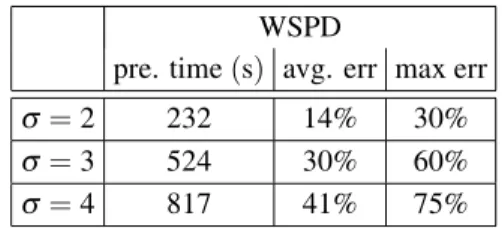
WSPD

pre. time(s) avg. err max err

σ=2 232 14% 30%

σ=3 524 30% 60%

σ=4 817 41% 75%

Table 8.Time for preprocessing on 1000 random points,

k=5,S=5,=5, varyingσ.

It turns out that higher values for σ induce a considerably higher precomputation since the grid size chosen by the grid pruning algorithm is smaller. But still, the quality deteriorates, as with the larger exponent in the cost function, even small perturbations might increase the cost considerably. So to keep the same error bounds, a smaller value forand/or a larger value forS

would have to be used.

7. Conclusions

We demonstrated that near energy optimal paths can be queried very efficiently even in large ra-dio networks. If the network is not too large, even slowly changing networks can be accom-modated. Nevertheless, many questions remain as to how such a technique could be used in real networks.

As long as the network is static, rather large net-works could be handled. For small netnet-works, the precomputed tables could even be replicated on all nodes. For large networks, the hash table can be distributed over the network. If paths are used for a long time₍seconds₎compared to the time needed for querying a path(milliseconds), even a centralized server for connection queries would be feasible. In that case, even occasional updates for inserting, deleting, or moving sta-tions would be feasible.

Finite maximum ranges can be accommodated easily by ignoring all connections that exceed this range in the path computations.

Distributed implementations that can accom-modate large and dynamic networks are a chal-lenge beyond the scope of this paper.

Contention of several routes using the same fre-quency bands at the same time are an issue not directly accessed by our shortest path model. However, forσ =2, our cost model minimizes the sum of the areas covered by the transmit-ters used in a path. This can have an indirect positive effect on contention.

Minimal total energy consumption does not guarantee fairness, i.e., it might happen that one station is used so often that its batteries are quickly drained. This effect can be mitigated in several ways. For example, rather than stor-ing fixed routes, we can simply store areas(e.g. squares₎where relay stations should be located. Any combination of points in these relay areas will yield an energy efficient path. In densely populated areas at least, one can balance energy consumption by picking random stations in each relay area. One can even explicitly take energy reserves or other priorizations into account.

References

[1] S. ARYA, D. M. MOUNT, Approximate range

search-ing, Computational Geometry: Theory and Appli-cations,17(2000), 135–152.

[2] S. ARYA, D. M. MOUNT, N. S. NETANYAHU, R. SIL

-VERMAN, A. WU, An optimal algorithm for

approx-imate nearest neighbor searching. Journal of the ACM,45(6) (1998), 891–923.

[3] N. BAMBOS, Toward Power-sensitive Network

Ar-chitectures in Wireless Communications: Concepts, Issues, and Design Aspects.IEEE Personal Comm.,

5(June 1998).

[4] R. BEIER, P. SANDERS, N. SIVADASAN, Energy

Op-timal Routing in Radio Networks Using Geometric Data Structures. Proc. of the 29th Int. Coll. on Automata, Languages, and Programming,(2002).

[5] M.DEBERG, M.VANKREFELD, M. OVERMARS, O.

SCHWARZKOPF, Computational Geometry:

Algo-rithms and Applications. Springer,(1997).

[6] P. B. CALLAHAN, S. R. KOSARAJU, A decomposition of multi-dimensional point-sets with applications to

k-nearest-neighbors and n-body potential fields.

Proc. of the 24th Ann. ACM Symp. on the Theory of Computation,(1992).

[7] P. B. CALLAHAN, S. R. KOSARAJU, Algorithms for Dynamic Closest Pair andn-Body Potential Fields.

Proc. of the 6th Ann. ACM-SIAM Symp. on Discrete Algorithm,(1995).

[8] J. L. CARTER, M. N. WEGMAN, Universal Classes of

Hash Functions.Journal of Computer and System Sciences,18(2) (1979), 143–154.

[9] T. CHAN, A. EFRAT, Fly cheaply: On the minimum

fuel consumption problem.Journal of Algorithms,

41(2) (November 2001), 330–337.

[10] A. EFRAT, S. HAR-PELED: Fly Cheaply: On the

Minimum Fuel Consumption Problem, Proc. of the 14th ACM Symp. on Computational Geometry,

[11] S. FUNKE, D. MATIJEVIC, P. SANDERS,

Approximat-ing Energy Efficient Paths in Wireless Multi-Hop Networks. Proc. of 11th European Symposium on Algorithms 2003 (ESA), number 2832 in LNCS, pp. 230–241, Springer.

[12] A. GOLDSMITH, S. B. WICKER(EDS.), Special Issue:

Energy-aware Ad Hoc Wireless Networks. IEEE Wireless Comm.,9(August 2002).

[13] C. E. JONES, K. M. SIVALINGAM, P. AGRAWAL, J. C.

CHEN, A Survey of Energy-efficient Network Pro-tocols for Wireless Networks.Wireless Networks,7

(July 2001).

[14] K. MEHLHORN, S. N ¨AHER, LEDA: A platform for

combinatorial and geometric computing. Cam-bridge University Press, 1999.

[15] K. MEHLHORN, S. N ¨AHER, Dynamic Fractional

Cas-cading.Algorithmica,5(1990), 215–241.

[16] D. PATEL, Energy in ad-hoc networking for the

picoradio. Master’s thesis, UC Berkeley, 2000.

[17] C. PETRIOLI, R. R. RAO, J. REDI(EDS.), Special

Is-sue: Energy Preserving Protocols.Mobile Networks and Applications,6(June 2001).

[18] T. S. RAPPAPORT,Wireless Communication. Prentice Hall, 1996.

[19] M. THORUP, U. ZWICK, Approximate Distance Or-acles. Proc. of 33rd Symposium on the Theory of Computation2001.

Received:May, 2007 Accepted:November,2007

Contact addresses: Stefan Funke, Domagoj Matijevi´c, Max-Planck-Institut f¨ur Informatik 66123 Saarbr¨ucken Germany e-mail:[email protected]

Peter Sanders Universit¨at Karlsruhe Fakult¨at f¨ur Informatik 76128 Karlsruhe Germany

STEFANFUNKEreceived his PhD in computer science from the Univer-sit¨at des Saarlandes, Germany in 2001. After spending some time at the Max-Planck-Institute f¨ur Informatik in Saarbr¨ucken and at the Univer-sity of Illinois at Urbana-Champaign as postdoctoral researcher, as well as at Stanford University as a visiting assistant professor, he is now a full professor at the Ernst-Moritz-Arndt-Universit¨at Greifswald, Germany. His research interests range broadly from theoretical to applied algo-rithmics, including areas like computational geometry, combinatorial optimization, and wireless networking.

DOMAGOJMATIJEVIC´received his PhD in computer science from the Universit¨at des Saarlandes, Germany in 2007. He is now a postdoctoral researcher at the Department of Mathematics, Josip Juraj Strossmayer University in Osijek, Croatia. His areas of interest include computa-tional geometry, approximation algorithms, wireless networking and combinatorial optimization.

PETERSANDERSreceived his PhD in computer science from Universit¨at Karlsruhe, Germany in 1996. After 7 years at the Max-Planck-Institute for Informatics in Saarbr¨ucken he returned to Karlsruhe as a full pro-fessor in 2004. In 2004 he was also awarded the Alcatel SEL Research Prize. He has more than 100 publications, mostly on algorithms for large data sets. This includes parallel algorithms(load balancing,...)