PyCatch: component based hydrological catchment modelling

(1)

PyCatch: COMPONENT BASED HYDROLOGICAL

CATCHMENT MODELLING

N. LANA-RENAULT1*_{, D. KARSSENBERG}2

1 _{Área de Geografía, Departamento de Ciencias Humanas, Universidad de La Rioja,}

26004 Logroño, España.

2 _{Department of Physical Geography, Faculty of Geosciences, Utrecht University,}

P.O. Box 80115, Utrecht, The Netherlands.

ABSTRACT.Dynamic numerical models are powerful tools for representing and studying environmental processes through time. Usually they are constructed with environmental modelling languages, which are high-level programming languages that operate at the level of thinking of the scientists. In this paper we present PyCatch, a set of components for process-based dynamic hydrological modelling at the catchment scale, built within the PCRaster Python framework. PCRaster Python is a programming tool based on Python, an easy-to-learn programming language, to which components of the PCRaster software have been added. In its current version, PyCatch simulates the processes of interception, evapotranspiration, surface storage, infiltration, subsurface and overland flow. The model represents those hydrological processes as a series of interconnected stores, and it is structured in such a way that the exchange of water fluxes between the stores is easily performed. The modular structure of PyCatch makes it easy to replace or adapt components (such as a snow melt component or a soil erosion and sediment transport component) according to the aim of the study.

PyCatch: modelización hidrológica a escala de cuenca con una estructura basada en componentes

(2)

procesos hidrológicos a partir de una serie de depósitos conectados entre sí, y está estructurado de tal manera que favorece el intercambio de flujos de un depósito a otro. La estructura modular de PyCatch permite reemplazar o añadir componentes fácilmente (por ejemplo, fusión de nieve o erosión de suelo y trans-porte de sedimentos) en función de los objetivos del estudio.

Key words:dynamic modelling, environmental modelling language, PCRaster Python, hydrological model.

Palabras clave: modelos dinámicos, lenguaje de modelización ambiental, PCRaster Python, modelo hidrológico.

Enviado el 15 de enero de 2013 Aceptado el 2 de febrero de 2013

* Correspondencia: Área de Geografía, Departamento de Ciencias Humanas, Universidad de La Rioja, 26004 Logroño, España. E-mail: [email protected]

1. Introduction

Environmental scientists are concerned with the understanding of how living organisms and their non-living environments function and interact (Mulligan and Wainwright, 2004). This understanding may contribute to the sustainable management of these systems upon which, eventually, humans depend. Also, it makes scientists such as hydrologists, ecologists, soil scientists or climatologists capable of predicting the impacts of events that have not yet happened or happened in the past. Hydrologists, for instance, need to know how the hydrological system works in order to explore the direction of changes due to changes in climate or land use and to predict how those changes in the system will affect water supply.

Numerical modelling can be a powerful means for representing and communicating our understanding of environmental systems. Models have a scientific value since they can be used to conceptualize system processes and to develop and test hypotheses concerning these processes. They are also important for management because they can be used as virtual laboratories to explore the outcomes of (numerical) experiments: models enable the assessment of changes in systems, and the prediction of their future evolution given these changes. A model of the environment is a representation of the natural processes that usually include spatial components that change over time. Thus, models are mostly spatially explicit and their temporal behaviour is simulated using rules of cause and effect, for that reason they are called dynamic models (Wesselling et al., 1996).

(3)

connectivity still needs to be fully incorporated in our conceptual (but also computer simulations) models. This means that models also need to evolve continuously and scientists should be able to adjust or update them without too many difficulties. For this, they need a model construction tool (i.e., a modelling language) suitable for people who have the knowledge of the environmental processes but are not specialists in programming. As stated by Karssenberg (2002), for this tool to be efficient, it should i) operate at the level of thinking of the scientists, i.e., use components resembling environmental concepts with entities and high level operators that represent natural processes; ii) support re-use and combination of program code; iii) provide a generic approach to model construction; iv) hide technical details from the user; v) result in short development times, vi) minimize programming errors; and vii) minimize run times.

The range of existing tools for environmental model construction is large but very few fulfill all the requirements mentioned above: system program languages (C++, FORTRAN) allow any model to be constructed from scratch, but they are difficult for non-programmers to use; technical computing languages (e.g., MATLAB) are powerful tools for numerical computation but they often lack a generic approach for temporal modelling, and the coupling with spatial databases is difficult; graphical languages (e.g., ModelMaker, STELLA) include process modelling and can be easily used without programming knowledge but do not provide spatial operators; modelling languages incorporated in Geographical Information Systems (GIS) are spatial by definition and a good alternative for developing environmental models but many of them often deal with static spatial data so they are not suitable for dynamic modelling. Therefore, new languages designed for the specific purpose of environmental spatio-temporal modelling were developed. These so-called environmental modelling languages (EML) are high level programming languages embedded in a GIS that provide a set of functions capable to operate on spatio-temporal data, database management and visualization routines (Wesselling et al., 1996; Karssenberg, 2002). Recently, the PCRaster Python extension and PCRaster Python frameworks were developed (Karssenberg et al., 2007; Schimtz and Karssenberg, 2009; PCRaster, 2013) as a powerful tool for supporting environmental model construction. The PCRaster Python extension enables the use of PCRaster modelling engine from Python (Python, 2013), a generic and easy-to-learn programming language. More details on the PCRaster Python extension and frameworks are given in the next sections.

(4)

model from scratch; instead, we used pre-programmed blocks of code and combined them to build up a model tailored to our aim study. Here, we first explain briefly the concept of dynamic modelling; then we present the mathematical description of PyCatch; and finally we describe how the model was built within the PCRaster Python framework, emphasizing on the capacity of such tool to improve program efficiency and quality.

2. Dynamic spatial environmental modelling

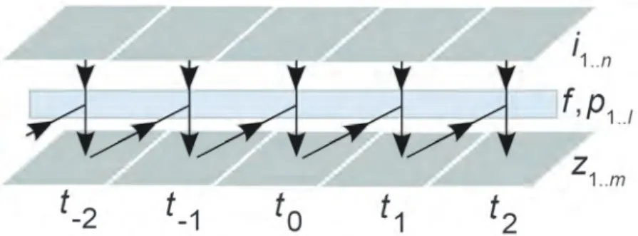
The property of a dynamic model is that it is run forward in time, i.e., the state of the model at time t+1 is defined as a function of its state in a previous time step t. The concept of dynamic modelling has been described elsewhere (e.g., Beck et al., 1993; Van Deursen, 1995; Wesseling et al., 1996) and can be represented by the following equation, which is illustrated in Fig. 1:

for each t (1) Each landscape attribute that is modelled is represented by a state variable z_k, k= 1.. m. The change in the attributes z_1.._mover time is given by the functional fassociated with the parameters p_1.._l. The so-called transition function f can be an update rule, explicitly specifying the change of the state variable over the time slice (t, t+1); a probabilistic function, when the model behaviour is better described as a stochastic process; or a derivative of a differential equation describing the change of the state variables as a continuous function (Karssenberg and de Jong, 2005a). The inputs to the model i_1.._nare also called disturbances. They can be, for instance, incoming rainfall in a hydrological model or a vegetation map. Boundary conditions are also regarded as inputs. Note that z_1.._m, i_1.._nand p_1.._lmay be defined in two- or three- spatial dimensions. In most environmental models, the transition function f includes a set of functions f_1.._jdescribing the complex interactions between variables and inputs, and this is often referred to as the model structure. 3. Mathematical description of PyCatch

PyCatch is a set of process-based distributed hydrological model components aimed at simulating the effect of vegetation recovery on stream flow response in small catchments.

(5)

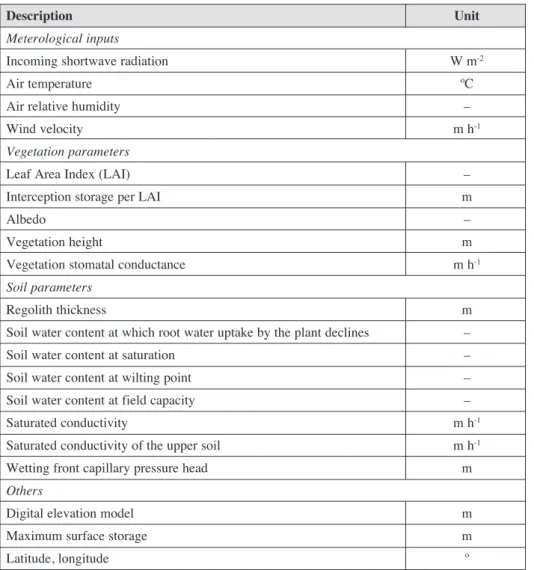
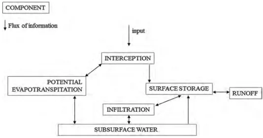
It is dynamic because it is designed to operate over successive short time steps (e.g., 1 hour) in order to get a detailed shape of the stream flow hydrograph. The model describes the processes of interception, evapotranspiration, surface storage, infiltration, subsurface and overland flow with process-based equations that use spatially and temporally distributed field data. In this first version, snow melt was not considered because our study was carried out in the Spanish Pyrenees, where most of the hillslopes affected by land abandonment and subsequent expansion of vegetation are located below 1600 m a.s.l., i.e., below the 0ºC isotherm during the cold season. Fig. 2 shows a schematic overview of the model, with boxes representing a particular subdomain of the hydrological system, and table 1 lists all input variables and parameters required for the model application.

Table 1. Main inputs and parameters for PyCatch.

Description Unit

Meterological inputs

Incoming shortwave radiation W m-2

Air temperature ºC

Air relative humidity –

Wind velocity m h-1

Vegetation parameters

Leaf Area Index (LAI) –

Interception storage per LAI m

Albedo –

Vegetation height m

Vegetation stomatal conductance m h-1

Soil parameters

Regolith thickness m

Soil water content at which root water uptake by the plant declines –

Soil water content at saturation –

Soil water content at wilting point –

Soil water content at field capacity –

Saturated conductivity m h-1

Saturated conductivity of the upper soil m h-1

Wetting front capillary pressure head m

Others

Digital elevation model m

Maximum surface storage m

(6)

3.1. Interception and evapotranspiration

Precipitation (P, [m h-1_{]) can either be intercepted by vegetation or directly reach} the soil. The part of the precipitation that it is intercepted by vegetation (P_int[m h-1_] depends on the canopy gap fraction f_gap:

(2) (3) where kis the light extinction coefficient [–] and LAIthe leaf area index [–]. Here we took k= 0.5 (Brolsma et al., 2010). The intercepted water evaporating from the canopy is computed using the Penman-Monteith equation for potential evaporation of open water, E₀[m h-1_{]. The actual interception (I, [m h}-1_{]) at time t}_{is limited by the maximum} interception capacity of the vegetation, and the water that was not evaporated in the previous time step and is still present in the canopy. The precipitation that reaches the ground as throughfall (P_net, [m h-1_{]) is}

(4) Evapotranspiration was calculated using the Penman-Monteith (Allen et al., 1998) equation for potential evapotranspiration (E_p, [m h-1_]):

(7)

(5)

In Eq. 5, λ[J kg-1_{] is the latent heat of vaporization of water, R}

n[W m

-2_{] is the net} radiation, δ [Pa K-1_{] is the slope of the saturation vapour pressure-temperature} relationship,ρ_a[kg m-3_{] is the mean air density at constant pressure, c}

p[J kg

-1_K-1_{] is the} specific heat of the air at constant pressure, υ [Pa] is the vapour pressure deficit of the air, γ[Pa K-1_{] is the psychrometric constant, r}

cand raare the canopy (or surface) and

aerodynamic resistances [h m-1_{], respectively.}

Net radiation (R_n) was determined taking into account the shading effect of the relief imposed by the digital elevation model (DEM) and the land surface inclination. For the latter we followed the same approach used in POTRAD 5.0 (Dam, 2000).

For each time step t, first evaporation takes place from the canopy using the Penman equation for open water conditions, i.e., with r_c= 0. No transpiration occurs as intercepted water evaporates. Soil evapotranspiration (ET, [m h-1_{]) depends on the} evaporation taken from canopy (I):

(6) When there is no water in the canopy to be evaporated (I= 0), transpiration is at potential evapotranspiration rate E_p. E_p is additionally controlled by the vegetation stomatal conductance (g_s,max, [m h-1_{]) which depends on the soil water content (θ, [–]).} To account for this effect, a soil moisture reduction function f(θ) based on Feddes et al. (1978) and Brolsma et al. (2010) was included:

(7)

(8)

withθ_lpthe soil water content at which root water uptake by the plant declines and θ_wpthe soil water content at wilting point. The actual evapotransiration from the soil (T, [m h-1_]) is limited by the soil potential evapotranspiration (ET) and the water available in the soil:

(9)

3.2. Soil water balance and subsurface flow

(8)

(Inf_p_,[m h-1_{]), which is related to the cumulative infiltration F}_{[m] as follows (Chow et} al., 1988):

(10)

where K_inf[m h-1_{] is the saturated conductivity of the upper soil,}_φ_{is the wetting front} capillary pressure head, and Δθis the available pore space. The water that is infiltrated (Inf, [m h-1_{]) is limited by the potential infiltration rate and the water available for} infiltration above the soil surface Qs[m h-1_{] at time step t:}

(11) Soil water storage (G_t, [m]) at time stept is determined by the amount of water present in the soil in the previous time step (G_t_-1), soil evapotranspiration (T), infiltration (Inf), subsurface inflow from the upstream neighbouring cells (Qg_,i, [m h-1_{]) and the} subsurface outflow to the downstream cell (Qg_o, [m h-1_]):

(12) For each cell, subsurface flow (Qg, [m h-1_{]) to the downstream area is modelled} using Darcy’s law as follows:

(13) in which K_satis saturated conductivity [m h-1_{], L}_{[m] is the cell length and α}_{[–] is the} slope to the downstream neighbouring cell. Qgis routed over the local drain direction (ldd) map which simulates the flow of material over a gridded surface (here, the digital elevation model) according to the direction of the steepest downhill cell and a D8 algorithm (Burrough and McDonnell, 1998). When Gat time step texceeds the volume of soil pores, upward seepage (Qx, [m h-1_{]) occurs and is added to the surface water (Qs,} [m h-1_{]) as saturation excess overland flow:}

(14)

where s_th[m] is the soil thickness and θ_sat[–] is the soil water content at saturation. 3.3. Overland flow

For each time step t, overland flow (Qr, [m h-1_{]) is determined by the precipitation} that reaches the ground (P_net), the exfiltrated water (Qx), the water available at the soil surface (Qs) in the previous time step, and infiltration (Inf):

(9)

The overland flow measured at the outlet of the catchment is the cumulative value of Qrrouted over the ldd. No travel times were considered because we assumed that Qr is brought to the outlet point at the same time.

4. The implementation of PyCatch in PCRaster Python

Python is an interpreted, object-oriented, extensible and free distributed programming language. Its very simple syntax makes it attractive to researchers. However, to make it useful for environmental modelling, additional spatio-temporal functionality is necessary. The PCRaster Python extension (Karssenberg et al., 2007) has taken this functionality from the PCRaster software (PCRaster, 2013), offering i) data structures containing spatial and temporal entities and operators, ii) a script framework that can be used for temporal modelling, and iii) an interactive visualization routine.

4.1. Entities, operators, functions and syntax

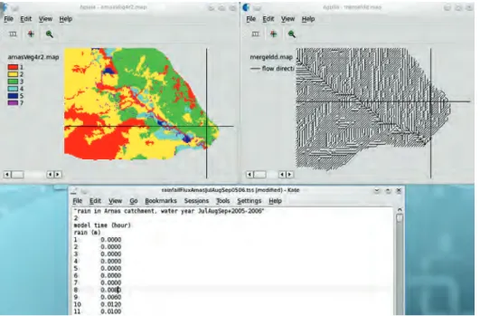
Environmental modelling languages need to operate at the conceptual level of thinking of the scientist. For this, they need to deal with entities and operators representing environmental attributes, dimensions and processes. In the PCRaster environmental modelling language, entities are raster maps of spatio-temporal attributes, time-series of temporal non-spatial data, and look up tables. Map entities are assigned a type according to the properties of the data they represent: they can be Boolean, nominal or ordinal for classified data (e.g., outlflow point, types of vegetation); scalar and directional for continuous data (e.g., temperature, elevation, aspect); and local drain direction for drainage networks. Fig. 3 shows three examples of PCRaster entities used in our study case: in the upper panels, two raster maps of the catchment (containing vegetation and the local drain direction); and a rainfall time series in the bottom panel.

The PCRaster language contains a set of operators and pre-programmed functions operating on these entities, including a large range required for environmental modelling such as hillslope and catchment analysis or routing functions to model transport of material over the local drain direction. Functions are grouped into (Burrough and McDonnell, 1998): point functions; direct and entire neighbourhood functions; neighbourhood defined by a given topology functions; time functions for retrieving and storing temporal data in iterative dynamic modelling (e.g., hydrographs at specific locations); and functions calculating descriptive statistics (Karssenberg and de Jong, 2005a, b). In PCRaster Python, all these PCRaster functions are callable from Python through the PCRcalc Python extension.

(10)

result=function (2.0 * input1…n)

where functionis one of the functions of the language,having the input variable

input_1…n multiplied by 2.0, resulting in the output variable result. All functions check the data type of their inputs, and might change their behaviour depending on the data type of the input variable (van Deursen, 1995). Also, the functions can be nested in one statement:

result=function(anotherFunction (2.0 * input_1…n), input_1…m)

where the result of anotherFunction is the input variable of another PCRaster function.

With these data structures and functions embedded, Python becomes a powerful tool for map algebra and static modelling. For instance, in PyCatch, creating a map containing runoff is done as follows:

ldd = readmap(‘ldd.map’)

discharge = accuthresholdflux (ldd, throughfall, availableSurface)

report (discharge, ‘runoff.map’)

(11)

The arguments of the function accuthresholdflux are three variables: the local drain direction (ldd) which is a map directly read from disk; and two variables referring to throughfall and the water available at the soil surface, calculated by the model (see Eq. 15). The accuthresholdflux function calculates the input of material downstream over a local drain direction network when a transport threshold is exceeded (here, availableSurface), and assigns it to discharge. The reportfunction writes the variabledischargefrom memory to the hard disk and stores it under the file name ‘runoff.map’. For model building, the functions can be glued together in a model script structured in sections. Sections are important in environmental modelling language because they tell the computer how to execute the model but also help the user to organize and structure the components of the model (Wesselling et al., 1996). 4.2. The script for dynamic modelling

Environmental models are dynamic models that need a framework for modelling changes over time. In the PCRaster language, the two main sections for building a sequential dynamic model are (Wesseling et al., 1996):

– The initial section, which sets the values of maps and non-spatial attributes representing the state of the model at the start of the model run.

– The dynamic section, which is an iterative sequential section and loops for the number of time steps defined in the model, and. For each time step t, it defines a set of operations that result in Map_1…_t. The results of time step tare the input values for time step t+1, and so on.

(12)

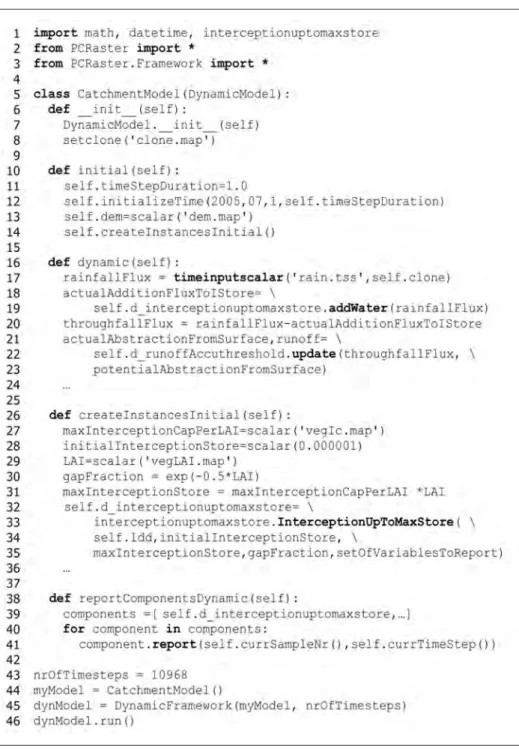
Based on these concepts, the PCRaster Python tool provides a framework as a Python class to construct and run dynamic models. Table 2 shows the template script of this framework. In the first line of the example script, the class definition is imported to the Python script, together with all other components of the PCRaster Python library. Below, the class UserModelis defined, with a given initialization and the definition of the initial and dynamic functions, also called methods. The __init__method is used to instantiate (i.e., to create) the objects of the class. Here, setting the map attributes (e.g. number of rows and columns and cell size) is done by using setclone. In the

initial method the state of the model at t=0 is defined. The dynamic method defines the change of the variables over one time step, and it is executed iteratively for a defined number of time steps. The execution of the model defined in the framework is done in the last statements. Here, the number of time steps is given as second argument to the framework constructor in line 13.

As within PCRaster, the dynamic section contains the operations representing the temporal behaviour of the model. In PyCatch, it includes calls to modules each represen-ting a particular hydrological process, here interception, evapotraspiration, infiltration, subsurface and overland flow. As shown in Fig. 2, these processes are represented as a series of interconnected stores. The output flow from one store may be determined by the input flow to that store. We need therefore a model structure capable of embodying such exchange of information. This is a key concept in complex environmental modelling and it can be done in a straightforward manner with the PCRaster Python framework. Unlike the original PCRaster language, PCRaster Python allows to use control flow constructs provided by Python, such as functions, built in types and classes (Python, 2013). Model code, for instance, can be embedded in a function, and this function can be called in a script as many times as necessary, minimising the amount of code in the script. The advantage of embedding code in a function is that the code can be easily re-used, but also that another person can call the implementation of that function in a different script, improving thus the property of shareability (Karssenberg et al., 2007). Similarly, functions can be embedded in classes that combine functions and variables. It is easy then to embed additional functions in a script, by using existing extensions, writing new extensions or developing new modules written in Python. In this way, large and complex models can be written keeping the code readable.

(13)

(14)

In the first lines, the components used in the model are imported. The model is created by defining the standard Python class for dynamic modelling, here CatchmentModel

(line 5), with the required initial and dynamic methods used in the dynamic framework. The

initialmethod (line 10) defines the time step duration, the time at which the model run start, and the digital elevation model, which is a file read from disk and assigned to the variable self.dem. With the selfprefix Python reads them as member variables. The

initialis evaluated once at the start of the model. In our study, we used time step of 1 hour and run the model for the hydrological year 2005-2006, starting three months before, on the 1st _{of July 2005. The}_initial _{method also includes the function}

CreateInstancesInitial, which is defined later on in the script, and is used to instantiate the components of the model.

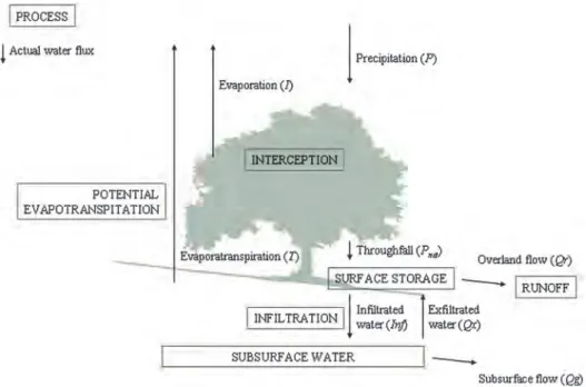
The dynamicmethod contains the set of operations included in the transition function fin Eq. 1 and represented in the hydrological system depicted in the flow diagram of Fig. 4. In this section the exchange of fluxes is done, as the outcome of one component feeds another component, which in turn feeds another one and so on. In the case of interception, rainfall is imported through the timeinputscalaroperation in line 17. For every time step, this operator links the value read from the time series ‘rain.tss’ to the map

rainfallFlux. The water added to the interception store is calculated by passing as an argument rainfallFlux in the function addWater, contained in the component

interceptionuptomaxstoreand invoked in line 19. The result of the function is used

to calculate throughfallFluxin the next line. In the same way, throughfallFlux

is used to calculate the runoff, by passing it as an argument in the function update

contained in the runoffAccthresholdcomponent, invoked in line 22.

(15)

In the CreateInstancesInitialmethod, all the components that are used in the model need to be initiated. In the case of the interception store, this is done in lines 27 to 35. The initial interception store is set to a very small value, and the Leaf Area Index and maximum interception capacity per Leaf Area Index are read from disk. These variables are used as inputs to calculate the gap fraction and the maximum interception store which, together with the initial interception store, instantiate the d_interceptionuptomaxstore

component. Finally, in the reportComponentsDynamicmethod (line 38), the report

function is invoked for every component, allowing the results of each component to be written to disk.

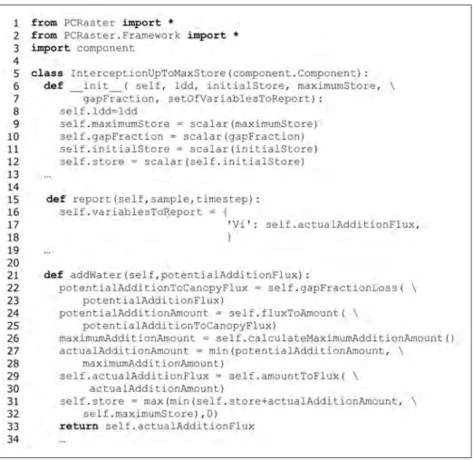
Table 4 gives a simplified version of the script for the interception component. The class InterceptionUpToMaxStore is instantiate in line 6. The function

addWater, referred above, is defined in line 21, and the function reportin line 15.

Here, the result of the function addWater, ie, actualAdditionFlux(line 33), is stored as ‘Vi’ in memory disk.

(16)

4.3. The interactive visualization routine

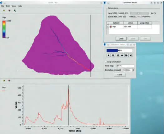
The spatio-temporal data stored on the hard disk can be displayed with the Aguila visualization tool integrated within PCRaster. Aguila (Pebesma et al., 2007) allows prompt visualization of model inputs and outputs. For temporal data, map views or time series can be animated through time. Fig. 5 shows screenshots of how Aguila visualizes the runoff calculated with PyCatch. The bottom panel corresponds to the time series of the runoff at the outlet of the catchment for one hydrological year. The location of the outlet is shown by the cross in the map view (the upper left panel). The user can browse the map to show time series of other locations. The value for a specific location and a specific time step is shown in the cursor window (the upper right panel). Here, we selected time step 6475, which corresponds to 27th of March 2006 at 18:00, when the maximum discharge for that hydrological year was reached, and is shown in the time series plot with a vertical line. The player at the bottom can be used to animate all the panels over time.

Figure 5. Screenshots of Aguila visualizations of the modelled runoff: map view of the catchment where the outlet is shown by a cross (upper left panel); time series with the runoff

at the outlet of the catchment for one hydrological year (bottom panel); cursor window (upper right panel) for the selected outflow and time step, which is shown by a vertical

(17)

5. Conclusions

When modelling environmental processes, scientists are able to understand observations and develop and test theory. The environment is a complex system under continuous change including important spatial interactions; therefore environmental processes need to be simulated on a spatial domain and by dynamic modelling. For this, scientists need a modelling language capable of representing such complexity in the simplest possible way. The PCRaster Python environmental modelling language is a recently developed programming tool based on Python, an easy-to-learn high-level programming language, to which components of the PCRaster software have been added. This makes PCRaster Python a powerful tool for supporting spatio-temporal modelling.

In this study, we presented the mathematical description of the process-based hydrological model PyCatch designed for small catchments located at mid altitudes mountain areas. We also explained how it has been implemented in PCRaster Python to illustrate the efficiency of the language for constructing complex environmental models. The modular structure of PyCatch makes it easy to replace or adapt modules (or components) according to the aim of the study. For instance, a snow melt module could be easily added when running the model for high elevation catchments. Similarly, soil erosion and sediment transport could also be included in the model without too much effort, by incorporating new modules based on existing erosion models.

Acknowledgements

This research was conducted with the support of INDICA projects CGL2011-27753-C02 and C01, financed by the Spanish Ministry of Economy and Competitiveness, and RESEL, financed by the Spanish Ministry of the Environment. N. Lana-Renault was the recipient of a research contract (Juan de la Cierva programme) funded by the Spanish Ministry of Sciences and Innovation. Oliver Schmitz and Kor de Jong are grateful thanked for their help.

References

Allen, R.G., Pereira, L.S., Raes, D., Smith, M. 1998. Crop evapotranspiration. FAO Irrigation and Drainage Paper No. 56, FAO, Roma.

Beck, M.B., Jakeman, A.J., Mcaleer, M.J. 1993. Construction and evaluation of models of environmental systems. In Modelling Change in Environmental Systems,M.B. Beck, A.J. Jakeman, M.J. McAleer (Eds.), Wiley, New York, pp. 3-35.

Burrough, P.A., McDonnell, R.A. 1998. Principles of Geographical Information Systems. Oxford University Press, Oxford.

Bracken, L.J., Croke, J. 2007. The concept of hydrological connectivity and its contribution to understanding runoff-dominated geomorphic systems. Hydrological Processes 21, 1749-1763. Brolsma R.J., Karssenberg, D., Bierkens, M.F.P. 2010. Vegetation competition model for water and light limitation. I: Model description, one-dimensional competition and the influence of groundwater. Ecological Modelling221, 1348-1363.

(18)

Dam, O. 2000. Modelling incoming Potential Radiation on a land surface with PCRaster: POTRAD5.MOD manual. Utrecht University, Utrecht, 6 pp.

Feddes, R.A., Kowalik, P., Jaradny, H. 1978. Simulation of field water use and crop yield.

Simulation Monographs, Pudoc, Wageningen, 189 pp.

Karssenberg, D., 2002. The value of environmental modelling languages for building distributed hydrological models. Hydrological Processes16, 2751-2766.

Karssenberg, D., De Jong, K. 2005a. Dynamic environmental modelling in GIS: 1. Modelling in three spatial dimensions. International Journal of Geographical Information Science19, 559-579.

Karssenberg, D., De Jong, K., 2005b. Dynamic environmental modelling in GIS: 2. Modelling error propagation. International Journal of Geographical Information Science19, 623-637. Karssenberg, D., De Jong, K., Van der Kwast, J. 2007. Modelling landscape dynamics with

Python. International Journal of Geographical Information Science21, 483-495.

Mulligan, N., Wainwright, J. 2004. Modelling and model building. In Environmental Modelling: Finding Simplicity in Complexity, N. Mulligan, J. Wainwright (eds.), John Wiley, Chichester, 430 pp.

PCRaster, January 2013. PCRaster internet site. Available online at: http://www.pcraster.eu/. Pebesma, E.J., De Jong, K., Briggs, D. 2007. Interactive visualization of uncertain spatial and

spatio-temporal data under different scenarios: an air quality example. International Journal of Geographical Information Science21, 515-527.

Python, January 2013. Python Programming Language internet site. Available online at: http:// www.python.org.

Schimtz, O., Karssenberg, D. 2009. Framework for Spatio-Temporal Modelling: Supporting Deterministic and Stochastic Modelling, Data Assimilation and Model Calibration. Faculty of Geosciences, Utrecht University, Utrecht, 24 pp.

Van Deursen, W.P.A. 1995. Geographical Information Systems and Dynamic Models. Koninklijk Nederlands Aardrijkskundig Genootschap/Faculteit Ruimtelijke Wetenschappen. Universiteit Utrecht, Utrecht.

Wesseling, C.G., Karssenberg, D., van Deursen, W.P.A., Burrough, P.A. 1996. Integrating dynamic environmental models in GIS: the development of a Dynamic Modelling language.

Transactions in GIS1, 40-48.

Appendix. List of symbols for PyCatch

Symbol Meaning Unit

c_p specific heat of the air at constant pressure J kg-1_K-1 E_p Penman-Monteith potential evapotranspiration m h-1 E₀ potential evaporation for open water conditions m h-1 ET potential soil evapotranspiration m h-1

F cumulative infiltration m

f_gap canopy gap fraction

-G soil water storage m

g_s,max stomatal conductance m h-1

(19)

Symbol Meaning Unit

Inf actual infiltration rate m h-1

Inf_p potential infiltration rate m h-1

k light extinction coefficient

-K_inf saturated conductivity of the upper soil m h-1

K_sat saturated conductivity m h-1

L cell length m