Vol. 4, No. 4, 2011, 370-423
ISSN 1307-5543 – www.ejpam.com
Euler and Divergent Series
Victor Kowalenko
ARC Centre of Excellence for Mathematics and Statistics of Complex Systems, Department of Math-ematics and Statistics, The University of Melbourne, Victoria 3010, Australia
Abstract. Euler’s reputation is tarnished because of his views on divergent series. He believed that all series should have a value, not necessarily a limit as for convergent series, and that the value should remain invariant irrespective of the method of evaluation. Via the key concept of regularisation, which results in the removal of the infinity in the remainder of a divergent series, regularised values can be evaluated for elementary series outside their circles of absolute convergence such as the geometric series and for more complicated asymptotic series called terminants. Two different techniques for eval-uating the regularised values are presented: the first being the standard technique of Borel summation and the second being the relatively novel, but more powerful, Mellin-Barnes regularisation. General forms for the regularised values of the two types of terminants, which vary as the truncation parameter is altered, are presented using both techniques over the entire complex plane. Then an extremely accu-rate and extensive numerical study is carried out for different values of the magnitude and argument of the main variable and the truncation parameter. In all cases it is found that the MB-regularised forms yield identical values to the Borel-summed forms, thereby vindicating Euler’s views and restoring his status as perhaps the greatest of all mathematicians.
2000 Mathematics Subject Classifications: 00A30, 01A45, 01A50, 01A65, 01A70, 03A05, 03B30, 30B10, 30B30, 30D20, 30E15, 30E20, 34E05, 34E10, 40A05, 40G10, 40G99
Key Words and Phrases: Absolute Convergence, Asymptotic Form, Asymptotics, Asymptotic Series, Borel Summation, Cauchy Integral, Cauchy Principal Value, Complete Asymptotic Expansion, Condi-tional Convergence, Divergent Series, Domain of Convergence, Dominant Series, Equivalence, Euler’s Constant, Gamma Function, Geometric Series, Grandi’s Series, Harmonic Series, Jump Discontinu-ity, Logarithmic Divergence, Mellin-Barnes (MB) Regularisation, Mellin Transform, Poincar´e Prescrip-tion, Recurring Series, RegularisaPrescrip-tion, Regularised Value, RenormalisaPrescrip-tion, Stokes Line, Stokes Phe-nomenon, Stokes Sector, Subdominant Terms, Terminant, Truncation, Truncation Parameter
1. Introduction
Despite being regarded as one of the four greatest mathematicians of all time, to this day Euler’s reputation is tarnished because of the views he held on divergent series. First, he believed that every series, both convergent and divergent, should be assigned a certain value,
Email addresses:vkowaunimelb.edu.au, vkowalnetspae.net.au
but because of the fallacies and paradoxes surrounding the latter type of series, he felt that such a value should not be denoted by the name sum[6]. Second, he believed that the value should be independent of the actual method or technique used to determine it. Later, when the foundations of analysis were laid down, initially by Abel and Cauchy, and then by Weierstrass (“the father of modern analysis”) and Dedekind, divergent series were virtually banished from the mathematical lexicon. Consequently, Euler’s reputation suffered. In fact, the extremely gifted Abel, who died at the tragically young age of 26, described divergent series as “the invention of the devil” and that it was “totally shameless to base any demonstration on them whatsoever”. As recently as 2007, in an article celebrating the tercentenary of Euler’s birth Varadarajan [32] wrote that whilst Euler certainly had some misconceptions regarding the summation of divergent series, his greatness on this topic was not appreciated for a century after his death when mathematicians began to consider the development of a general theory of divergent series [12]. Later in the same article he states that although in his opinion Euler had taken the first steps towards creating a true theory of divergent series, which is still lacking today, the situation is much more subtle than Euler could ever have anticipated. Unfortunately, he does not elaborate on exactly what he means by “more subtle”.
Over the past few centuries mathematicians have, for the most part, tended to steer clear from divergent series, but unfortunately, there is one discipline or field where series of this type abound— asymptotics. In this discipline special methods or techniques, e.g. steepest de-scent, Laplace’s method and the iterative solution to differential equations to name a few, are used to derive solutions in form of the power series expansions whose coefficients eventually diverge quite rapidly. Although it is not clear whether such expansions are always divergent, they are invariably truncated according to the Poincaré prescription or definition as described on p. 151 of Ref. [33]. Generally, this involves truncating an expansion after a few terms. Then one is left with an approximation to a given function, whose accuracy is dependent upon whether the variable in the expansion tends to a limit point, which is often zero or infin-ity. Hence, depending upon whether the limit point is zero and infinity, we say that a function “goes as” or “is approximately equal to” the truncated expression in the limit as such and such variable goes to zero or infinity. In other instances the Landau symbols ofO()ando(), or even
+. . . , are used to signify that the remaining terms dropped from the truncated expression can be bounded. This is fiction of course, because the remainder is only bounded as long as there is an optimal point of truncation[24]. Even more troubling is the fact that the domain over which an optimal point of truncation exists is often unspecified or even unknown. In fact, for most values of the variable there is simply no optimal point of truncation. So, we have the situation today where standard asymptotics represents an inexact, if not crude, mathematical discipline composed of truncated asymptotic expansions that suffer from the drawbacks of vagueness and severe limitation in accuracy and range of applicability as a result of an overly permissive Poincar´e prescription. It is no wonder that the discipline is frequently subject to derisory remarks from pure mathematicians in particular, who point out that mathematics is supposed to be an exact science.
theory, non-local solitary waves, fluid mechanics and a host of other fields[4, 5, 21, 29]have required improved methods aimed at obtaining meaningful corrections that lie beyond all orders of a standard asymptotic expansion. In addition to these applications, analysts have been engaged in developing exponentially improved asymptotics of special functions such as the confluent hypergeometric and gamma functions as described in Ch. 6 of Ref. [27]. For these exceptional and important problems standard asymptotic analysis is simply inadequate. Therefore, the sub-discipline or field known as exponential asymptotics or asymptotics be-yond all orders, also occasionally referred to as hyperasymptotics, has evolved. Whilst this field seeks to derive the terms in an asymptotic expansion that are neglected by the applica-tion of the Poincar´e prescription, as explained at the beginning to Sec. 3 here, it still suffers from the same problem in standard asymptotics, which is: how does one obtain meaningful values to divergent series? This is because frequently these subdominant terms are themselves divergent series. Worse still, they are usually masked by a divergent dominant series. Hence, in order to determine both contributions to the overall solution, we again require a theory of divergent series for only then will it be possible to determine the exact values of the original function, which is the ultimate goal of asymptotics. If such a methodology could be formu-lated, then asymptotics would be elevated to a true mathematical discipline eliciting precise answers. This would not only have a profound effect on mathematics, but also on physics and engineering.
2. Divergent Series
When one wishes to discuss Euler’s “unorthodox” views on divergent series, one is in-evitably drawn into a study of the geometric series for it is this series that was used as the basis for his views. We shall do likewise, although it should be pointed out that the series has a fascinating history of its own going way back to Archimedes, who used it to calculate the area under a parabola intersected by a line. This became the precursor to integral calculus.
Before the geometric series can be introduced, however, we first need to understand what is meant by a divergent series. In actual fact, there is no formal or rigorous definition of a divergent series. Instead, we must examine what a convergent series is. Then by a process of elimination, anything that is not a convergent series is regarded as being divergent. Copson’s definition[7]begins with the symbol ofa0+a1+a2+. . .+ak+. . ., which involves the sum of an infinite number of complex numbers. To assign a meaning to this symbol, he then considers the partial sums,s0,s1,s2,. . . , where each partial sum is given by
sk=a0+a1+a2+. . .+ak . (1)
If this sequence tends to a finite limits, then the infinite series is convergent with the value of the limit equal tos. That is,s=P∞k=0ak.
can be regarded as special cases of the geometric series, although the last example is now known as Grandi’s series since he was the first to provide a simplistic account of it in 1703∗. In particular, he noticed that bracketing the series as (1−1) + (1−1) +. . . appears to yield a limit of zero, while bracketing it as 1+ (−1+1) + (−1+1) +. . . appears to yield a limit of unity. Therefore, we see that there are two possible limits for the series. However, because one can bound the series, one does not get the impression that it is divergent. Nevertheless, according to Copson[7], the series is divergent. In fact, Grandi himself did not think that it summed to either value, but to 1/2 for various reasons, none of which would be considered a mathematical proof today. Leibniz went further by introducing a “law of justice”, which amounted to averaging the two possible limits. Consequently, the series is also known as Leibniz’s series.
It was Euler who gave what could be regarded as the first proper mathematical treatment of Grandi’s series. To do so, we express the series in Eq. (1) as the geometric series by replacing
akbyxk, wherexcan be any value. When the magnitude of xis less than unity, i.e. for|x|<1, the limitsequals 1/(1−x). The series is said to be absolutely convergent for these values ofx. E.g., forx=1/4, the series becomes 1+1/4+1/16+1/64+1/256+. . .=1/(1−1/4) =4/3. Thus, Archimedes was able to show that the area enclosed by a parabola and straight line is 4/3 times the area of the triangle inscribed within this area. If we replace x by the complex variable z(= x+i y), then |z| <1 represents the unit disk centred in the complex plane. Furthermore, if we put x equal to -1, then we find that s=1/2, but the series is no longer absolutely convergent, which means that it is invalid to use the limit value of 1/(1− x). Instead, Euler wrote the series in terms of−x as
1
1+x =1−x+x
2−x3+. . .+ (−1)kxk+ (−x) k+1
1+x . (2)
Then the main objection to the use of 1/(1+x)whenx=1 is that the final term or remainder cannot be disregarded ask goes to infinity. His idea was that since an infinite series has no last term, it could be neglected. Later, he used finite differences to attack the problem, but in reality his explanation would not be considered valid today. As a consequence, in time his belief that every series should be assigned a certain value came under attack and his reputation began to wane as indicated earlier.
According to Varadarajan[32], Euler had several different methods for summing divergent series, but most of all he used what is now known as Abel summation. This amounts to extending the limit inside the unit disk of absolute convergence to a domain with z= 1. Unfortunately, for more intricate examples of divergent series, e.g. akequal to(−1)kΓ(k+1), where Γ(k+1) =k!=k(k−1). . . 2·1, this method breaks down completely, which is why Euler referred to such series as divergent series par excellence. Unlike the geometric series, which we have already stated possesses a radius of absolute convergence equal to unity, the latter type of series possesses zero radius of absolute convergence. We shall return to these series later in this article.
Despite the tone of his papers, Euler expressed doubt in private correspondence over his methods for handling divergent series, but he never found a counterexample to Grandi’s series
∗History of Grandi’s Series.,
equalling 1/2. Then in 1771 Daniel Bernoulli, who had accepted the result, noticed that by inserting zeros into the series, one could obtain any value between 0 and 1. For example, he found that 1+0−1+1+0−1+. . .=2/3[12]. This is really counter-intuitive and a theory of divergent series would need to account for how the introduction of an infinite number of zeros can yield a different limit. It is precisely this type of result that Abel was referring to when criticising divergent series for producing fallacies and paradoxes. Worse still, if the zeros and minus ones are re-ordered so that the series becomes 1−1+0+1−1+0+1−1+. . ., then we would obtain a different limit. In this case the limit would be 1/3.
In 1799 more than a decade after Euler’s death, the situation became even worse when Callet pointed out to Lagrange that
1+z
1+z+z2 =1−z
2+z3−z5+z6+. . . , (3)
gives Grandi’s series forz=1, but now the limit is 2/3 instead of 1/2. Lagrange defended Euler by stating that the rhs of Eq. (3) is not a true power series since many powers are missing. When these are included by writing the series as
1+0·z−z2+z3+0·z4−z5+z6+0·z7−z8+. . . , (4)
the series reduces to 1+0−1+1+0−1+. . . forz=1, which as stated previously, was found by Bernoulli to yield a limit of 2/3. Whilst this may have silenced Callet, it is particularly alarming for applied mathematicians who derive divergent series in the form of asymptotic series for often such series are in the form wherezis a power of another variable. For example, the asymptotic series for the error function, which appears in Sec. 9, is actually in powers of −1/z2. The above would imply that those missing powers, namely the odd powers of 1/z, would have to be included in the analysis to obtain the limit.
Since Lagrange, many mathematicians have introduced various methods for summing divergent series. Most of these sum Grandi’s series to 1/2. Others motivated by Bernoulli’s treatment sum the series to another value, while a small minority take the safe option of not bothering to sum it at all. Therefore, the issue has become whether all the inconsistencies or apparent paradoxes that have been raised here can be resolved.
3. Regularisation
In 1993 my colleague T. Taucher and I carried out a numerical study into the complete asymptotic expansion of a particular case of a number theoretic exponential series, which we called the generalised Euler-Jacobi series [21]. Specifically, our investigation concentrated on the series,S3(a) =P∞k=0exp(−ak3), which represented the p/q=3 case. This series was found to possess unimportant constant terms, which were removed so that remaining terms or the tail denoted by T3(a) yielded an asymptotic expansion, which was composed of two
separate divergent series. One of these series denoted byT3K(a)was subdominant to the other, which was denoted byT3L(a). Specifically, we found that
T3(a) =T3L(a) +T
K
where
T3L(a) =2 ∞
X
k=0
(−1)k+1a2k+1 (2π)6k+4
Γ(6k+4)
Γ(2k+2) ζ(6k+4) , (6)
whilst the subdominant series was given by
T3K(a) = 2 p
π Γ(1
6)Γ( 5 6)
∞
X
n=1
e−p2z (6πna)1/4
∞
X
k=0
Γ(k+1/6) (4pz)k
× Γ(Γ(k+5/6)
k+1/2) cos p
2z−π
8− 3kπ
4
. (7)
In these resultsz= (2nπ/3)3a−1, whileζ(s)represents the Riemann zeta function.
Subdominance in an asymptotic expansion means that one of the component series pos-sesses an exponential factor that causes the entire series to vanish as the main variable tends to the limit point, which in the above example refers to either a → 0 or z → ∞. That is, in this limit the exponential factor of exp(−p2z) appearing in Eq. (7) becomes vanishingly small in comparison with the dominant series given in Eq. (6). It should also be noted that subdominant terms can become the dominant terms and vice-versa as the main variable ora
in the above example undergoes changes in its argument or phase. However, at the time we were only interested in real values ofa. As described in the introduction, subdominant terms such as those in Eq. (7) are said to lie beyond all orders of the dominant part of the expansion
[4, 5, 29]and are generally neglected by practitioners of standard asymptotics. Neverthe-less, we found that they were necessary for obtaining exact values of the series regardless of the size of a. For example, when the first fifteen terms of the dominant series and the first twenty-one terms of the subdominant series are subtracted from T3(a) with a equal to 0.2, one obtains a value of
T3(0.2)−T3L(0.2, 15)−T
K
3(0.2, 21) =−8.458 470 156 185 480· · ·×10−
7 . (8)
On the lhs of the above equation, we have introduced the truncation parameter N into the series given by Eqs. (6) and (7) to indicate that the sums overkhave been evaluated partially by setting N =15 in the first series and N = 21 in the second series. The value on the rhs now represents the combined remainder of two divergent series. By using our newly-discovered mathematical technique, we were able to evaluate the remainder ofT3L(a), which when subtracted from the right hand side (rhs) of the above equation yielded a value of −1.588955334· · · ×10−17. Then by applying the same technique to the expression for the remainder of the subdominant series T3K(a), we obtained the same value. The analysis was repeated for numerous values ofa ranging from 0.01 to 10. On each occasion we obtained the exact numerical values of the remainder for the subdominant series. Therefore, for the first time in the history of mathematics we had shown that a complete asymptotic expansion could be used to generate the values of the original function it represented. All the results from this spectacular study were eventually documented and discussed in Chs. 7 and 8 of Ref.
The mathematical technique mentioned in the previous paragraph is known today as Mellin-Barnes regularisation. At its heart lies the key concept of regularisation, which is defined as the removal of the infinity in the remainder of a divergent series so as to make the series summable. It is the absence of this concept that has resulted in the fallacies and paradoxes occurring in divergent series as described in the previous section. So, let us exam-ine how regularisation applies to the geometric series since it represents a generalisation of Grandi’s series. To do so, we write the geometric series as
k X
k=0
zk= ∞
X
k=0
Γ(k+1) z k
k! =plim→∞ ∞
X
k=0
zk k!
Z p
0
d t e−ttk . (9)
In obtaining the above equation we have multiplied the summandzk byk!/k!, substitutedk! by its more general form in terms of the gamma function and then introduced the integral representation for the latter. That is,Γ(k+1)has been replaced by its integral representation ofR0∞d t tkexp(−t).
Although the integral in Eq. (9) actually extends from zero to infinity, the upper limit has been replaced by the finite valuep, which we let go to infinity later. Since the resulting integral in the above equation is now technically finite, we can interchange the order of the summation and integration. In reality, an impropriety is occurring here, which will be explained shortly. Nevertheless, if we persevere with interchanging the order of the summation and integration, then we find that the summation is not only absolutely convergent, but it also represents the Taylor series expansion for exp(z t). Therefore, replacing the series by this limit, we find that Eq. (9) becomes
∞
X
k=0
zk= lim
p→∞
Z p
0
d t e−t(1−z)= lim
p→∞
−e− p(1−z)
1−z +
1 1−z
. (10)
When the real part of z is less than unity, i.e. ℜz<1, the first term in the last member of Eq. (10) vanishes and the series yields the finite value of 1/(1−z). Hence, we see that the same value is obtained for the series whenℜz<1 as for when lies in the unit disk of absolute convergence.
According to the definition on p. 18 of Ref.[33], this means that the series is conditionally convergent for ℜz<1 and|z|>1 . That is, it is not divergent, but it is also not absolutely convergent either. Forℜz>1, however, the first term in the last member of Eq. (10) yields infinity. Since we have defined regularisation as the process of removing the infinity so that the series becomes summable, we remove or neglect the first term of the last member of Eq. (10). Then we are left with a finite result that once again equals 1/(1−z). We shall call this result the regularised value of the series when it is divergent. Hence, for all complex values ofzexcept forℜz=1, we arrive at
∞
X
k=0
zk (
≡1(1−z), ℜz>1,
=1/(1−z), ℜz<1. (11)
the equals sign by the less stringent equivalence symbol on the understanding that we may be dealing with a series that is absolutely convergent for some values of the variable. As a result, we adopt the shorthand notation of
∞
X
k=N
zk=zN
∞
X
k=0
zk≡ z N
1−z . (12)
Obviously, such mathematical statements are no longer equations for it is simply invalid to refer to the above as an equation because the left hand side (lhs) is infinite when ℜz>1, while the right hand side (rhs) remains finite for these values of z. Instead, we shall refer to such results as equivalence statements or simply equivalences, for short. It should also be noted that the above notation is only applicable when the result for the regularised value of a divergent series is identical to the limiting value of the convergent series. This is not always the case as can be seen from the final example in Ch. 4 of Ref.[17].
An important property of the above result is that it is one-to-one or bijective for each value ofz in the principal branch of the complex plane. This is critical for developing a theory of divergent series since it means that each value ofzwill yield a unique regularised value, which is beginning to accord with Euler’s belief that each series has a specific value. Thus, there is now a possibility that the fallacies and paradoxes that led to the banishment of divergent series from the mathematical lexicon can start to disappear.
At the barrier ofℜz=1, the situation appears to be unclear. Forz=1 the last member of Equivalence (10) vanishes, which is consistent with removing the infinity due to 1/(1−z). For other values ofℜz=1, the last member of Eq. (10) is clearly undefined, which is expected because this line forms the border or boundary between the domains of convergence and divergence for the series. Because the finite value is the same to the right and to the left of the barrier or line atℜz=1 and in keeping with the fact that regularisation is effectively the removal of the first term in the last member or rhs of Eq. (10), we take 1/(1−z)to be the finite or regularised value whenℜz=1. Hence, Equivalence (11) becomes
∞
X
k=0
zk (
≡1/(1−z), ℜz≥1,
=1/(1−z), ℜz<1. (13)
Since the equals sign is less stringent than the equivalence symbol, we can replace the former symbol by the latter in the above result. Then we find that Equivalence (12) is valid for all values ofz.
The standard rules of differentiation and integration apply to an equivalence statement just as they would to an equation. That is, the regularised value has to be either differentiable or integrable in order to operate on the series. For example, differentiating the preceding result jtimes yields
∞
X
k=j
Γ(k+1) Γ(k−j+1) z
k−j (
≡(−1)jΓ(j+1)(1−z)j+1, ℜz≥1,
while if we replacezby−zand integrate from 0 toz, then we obtain
∞
X
k=0
(−1)kzk+1
k+1
(
≡log(1+z), ℜz≤ −1,
=log(1+z), ℜz>−1. (15)
The series in the above result is often used as a textbook example of conditional series, e.g. see p. 18 of Ref.[33]. If one putsz=1 , then one obtains
1−1/2+1/3−1/4+1/5−1/6+. . .=log 2 . (16)
On the other hand, by putting z=−1 in Equivalence (15), one obtains the logarithmically divergent and quite famous harmonic series of 1+1/2+1/3+1/4+. . .. This series, which, as described in Sec. 7, represents a very different prospect to regularise from the geometric series, was studied in great detail by Euler[13]. Unbeknownst to him at the time, in writing down the equation for the constant that now bears his name from the harmonic series, viz.
γ= lim
k→∞
1+1
2+ 1 3+
1
4+. . .+ 1
k−logk
, (17)
he was actually displaying for the first time ever a formula for regularising a divergent series.
4. Divergent Integrals
As discussed in Refs.[14, 17], the regularised value of a divergent series is analogous to the Hadamard finite part that arises in the regularisation of divergent integrals in the theory of generalised functions[10, 23]. As a typical example, let us consider the general integral representation of the gamma function that was used to derive Eq. (9). This is
Γ(α) = Z ∞
0
d x xα−1e−x . (18)
The above integral is convergent forℜα>0, but is divergent for all other values ofα.
The divergence in the above integral is associated with the lower limit. If the lower limit is replaced byεand the limit of ε→0 is taken, then the above integral can be evaluated by integrating by parts continuously so that afterkintegrations one finds thatℜ(k+α)>0. Then one obtainsΓ(k+α)/α(α+1). . .(α+k−1) = Γ(α)plus a whole lot of contributions such as −εαexp(−ε)/α , −εα+1exp(−ε)/α and so on. In accordance with regularisation, these infinities are omitted or removed, leaving onlyΓ(α), which is the same result for ℜα >0 . According to p. 32 of Ref.[23], the remaining term was called the “finite part” by Hadamard, who showed that it obeys many of the ordinary rules of integration.
To demonstrate the relationship between the finite part of a divergent integral and the regularised value of a divergent series, consider the following integral:
I= Z ∞
0
d x ea x= lim
p→∞
Z p
0
d x ea x= lim
p→∞
eap−1
a
For ℜa<0, the integral in Eq. (19) is convergent, yielding a value of −1/a. On the other hand, for ℜa>0, it is divergent, but removing the infinity or first term in the last member yields, once again, a finite part of−1/a. Now to connect the above result with regularisation of a divergent series, we write the integral in terms of an arbitrary positive real parameter, say
b, as
I= Z ∞
0
d x e−b xe(a+b)x = Z ∞
0
d x e−b x
∞
X
k=0
(a+b)kxk
k! . (20)
In obtaining this result we have employed the asymptotic method of expanding most of the exponential as described on p. 113 of Ref.[8]. Next we interchange the order of the summa-tion and integrasumma-tion. Because most of the exponential has been expanded, an impropriety has occurred. Evaluating the resulting integral yields a divergent series, depending, of course, on the values ofaandb. As a consequence, we have to replace the equals sign by an equivalence symbol in the final result. Hence, the integralI becomes
I≡
∞
X
k=0
(a+b)k k!
Z ∞
0
d x e−b x xk= 1 a+b
∞
X
k=1
(1+a/b)k . (21)
The series in the final member of the above result is merely the geometric series with the variable equal to(1+a/b). If we introduce the regularised value of the series, viz.
−(1+a/b)/(a/b), into the last member of the above equivalence, then we obtain the finite value of−1/aas we did when we evaluated the integral in Eq. (19). That is, by regularising the series in Eq. (21), we have found thatI≡ −1/a, which is identical to the direct evaluation of the divergent integral and removal of the infinity or the first term in the last member of Eq. (19). Hence, regularisation of a divergent series is equivalent to evaluating the finite part of a divergent integral.
convergence will possess vastly different properties than within the radius of absolute conver-gence. Moreover, whilst regularisation has been presented as a mathematical abstraction for obtaining the finite value of a divergent series so far, it is required in asymptotics for correcting the impropriety of the method used to obtain the expansion from the original function.
With regard to the issue of whether the appearance of divergent integrals and series in applications constitutes a breakdown in physics or mathematics, it is more than likely to be a combination of both when dealing with the very small such as the Planck scale in parti-cle physics and physical cosmology. However, before the physical issues can be tackled, the mathematics needs to be corrected first. At the moment it appears that the wrong sort of mathematics is being employed, which has resulted in the rather bizarre predictions being made by eminent cosmologists and particle theorists today. We shall consider the physicist’s approach to renormalisation and compare it with the mathematical concept of regularisation in a later section.
5. Grandi’s Series Revisited
Let us now return to Grandi’s series, which is obtained by putting z equal to -1 in the geometric series. From our study of the geometric series in the previous section we know that Grandi’s series is conditionally convergent, and not divergent according to Copson’s definition. Hence, the limit of the series is simply 1/(1-(-1)) or 1/2, a result which is entirely consistent with Leibniz’s law of justice. If it is not divergent, then how can the introduction of an infinite number of zeros affect the limit as Bernoulli found?
Before we can consider this question, we need to examine what happens when an infinite number of zeros is introduced into an absolutely convergent series. Therefore, we write the geometric series as
S(z) =1+0+z+0+z2+0+z3+0+z4+0+. . . . (22)
Since every second element is zero, we can expressS(z)alternatively as
S(z) = ∞
X
k=1
1−(−1)k
2
z(k−1)/2+ ∞
X
k=2
1+ (−1)k)
2
0k . (23)
The above result represents the sum of four separate series. Hence, separating each series we obtain
S(z) = 1
2pz
∞
X
k=1
zk/2− 1
2pz
∞
X
k=1
(−1)kzk/2+1
2 ∞
X
k=2
0k−1 2
∞
X
k=2
(−0)k . (24)
The last two terms in Eq. (24) vanish according to Equivalence (13), which now becomes an equation sincez=0. That is, the equivalence symbol can be replaced by an equals sign. Furthermore, for|z|<1 the first two series can be evaluated with the equation form of Equiv-alence (13). Then we find that
S(z) = 1
2pz
p
z
1−pz −
1 2pz
−pz
1+pz =
1
Hence, we see that the introduction of an infinite number of zeros into the geometric series has no effect on its limit when|z|<1.
Let us now consider the introduction of an infinite number of zeros into Grandi’s series as Bernoulli did. Then we can write the modified version of Grandi’s series as
S3(1, 0,−1) =1+0−1+1+0−1+. . .
=1+0+0+1+0+0+1+. . .
+0+0−1+0+0−1+0+. . . . (26)
That is, Grandi’s series represents the sum of two separate series,S3(1, 0, 0)andS3(0, 0,−1).
The first series in Eq. (26) can be written alternatively as
S3(1, 0, 0) = 1
3 ∞
X
k=0
1k+e2πik/3+e4πik/3 , (27)
while the other series can be expressed as
S3(0, 0,−1) =−1
3 ∞
X
k=0
1k+e2πi(k−2)/3+e4πi(k−2)/3
. (28)
Therefore, we see that both S3(1, 0, 0) and S3(0, 0,−1) are themselves the sums of three specific geometric series. In each case the first series yields a regularised value of infinity, but as we are interested in the sum ofS3(1, 0, 0)andS3(0, 0,−1), these infinities cancel.
In order to evaluate the other series in Eqs. (27) and (28), we introduce the rhs of Equiv-alence (13). Aszis equal to either exp(2πi/3)or exp(4πi/3)in these series, we haveℜz<1. Hence, the equivalence symbol can be replaced by an equals sign, resulting in an equation. Combining the regularised values of all the series gives
S3(1, 0,−1) =
1 3
1−e−4πi/3
1−e2πi/3 +
1−e−2πi/3
1−e4πi/3
= 2
3 , (29)
which is the identical result obtained by Bernoulli. In addition, if the series had been given by 1−1+0+1−1+0+. . ., then the series would have becomeS3(1,−1, 0), which is the sum ofS3(1, 0, 0)andS3(0,−1, 0). The limit of the latter series is given by
S3(0,−1, 0) =−1
3 ∞
X
k=0
1k+e2πi(k−1)/3+e4πi(k−1)/3
. (30)
By combining this result with the limit forS3(1, 0, 0), we arrive at
S3(1,−1, 0) =
1 3
1−e−2πi/3
1−e2πi/3 +
1−e−4πi/3
1−e4πi/3
. (31)
6. Recurring Series
As a result of the foregoing analysis, we can consider any periodically recurring series of the form where
Sk(a1,a2,a3, . . . ,ak) =a1+a2+. . .+ak+a1+a2+. . .+ak+. . . . (32)
From the previous section we know thatSk(a1,a2,a3, . . . ,ak)can be expressed as a finite sum of series involving zeros and one. That is, the above can be written as
Sk(a1,a2,a3, . . . ,ak) =a1Sk(1, 0, 0, . . . , 0) +a2Sk(0, 1, 0, . . . , 0) +. . .
+ akSk(0, 0, 0, . . . , 1) . (33)
Each series on the rhs of Eq. (33) possesses an infinite sum over unity, just as in Eqs. (27) and (28). In the preceding cases we found that they eventually cancelled each other when evalu-ating the limits forS3(1, 0,−1)andS3(1,−1, 0). In the above result the sums over unity will cancel each other if and only ifPkj=1aj=0. Otherwise, one obtains infinity. Hence, we need
to make this assumption or condition to obtain a finite limit forSk(a1,a2,a3, . . . ,ak). In addi-tion, if we denoteSk(0, . . . ,ij, . . . , 0)as the series composed of zeros and ones, where the ones only appear at the j-th position of each cycle ofkterms, e.g.S3(0, 12, 0)has unity appearing
at the second position of every triple (0,1,0), then the above equation can be represented as
Sk(a1,a2,a3, . . . ,ak) = k X
j=1
ajSk(0, 0, . . . , 1j, . . . , 0)
= 1
k k X
j=1
aj k−1
X
l=1
∞
X
n=0
e2(n−j+1)lπi/k . (34)
The infinite sum over n can be removed by introducing the rhs of Equivalence (13) except that becauseℜexp(2lπi/k)<1 for all values ofl in the above result, the equivalence symbol can be replaced by an equals sign. Then Eq. (34) reduces to
Sk(a1,a2,a3, . . . ,ak) = i
2k k−1
X
l=1
1 sin(lπ/k)
k X
j=1
aje−(2j−1)lπi/k . (35)
Therefore, we arrive at a finite double sum that is very much dependent upon the values of theaj.
It should be noted that in Eq. (35) theaj need not necessarily be real. That is, they can be complex provided thatPkj=1aj=0. On the other hand, if they are purely real, then Eq. (32) can be simplified even further because the real part of the final sum, viz. the sum over j, must vanish. Therefore, in this case Eq. (35) yields
Sk(a1,a2,a3, . . . ,ak) = a1
2
1−1
k
+ i
2k k−1
X
l=1
× k X
j=2
aj
sin((2j−1)lπ/k)
sin(lπ/k)
. (36)
If we leta1=1,a2=0,a3=−1, andk=3 in the above equation, then, as expected, we find that
S3(1, 0,−1) =2/3, while fora1=1,a2=−1,a3=0, andk=3, we find thatS3(1,−1, 0) =1/3. For a more complicated series such asS4(3, 2,−4,−1), we obtain a limit value of 9/4.
Since we have seen that Grandi’s series is conditionally convergent rather than divergent, we now turn to the question of who is correct: Callet or Lagrange? In actual fact, both are correct, but for different reasons. First, we note that Grandi’s series admits an infinite number of encodings. To see this more clearly, consider the following series:
lim
z→1S(z) =zlim→1(1−z
p)
1+zq+z2q+z3q+. . .=lim
z→1(1−z
p)X∞
k=0
zqk, (37)
where bothℜpandℜqare greater than zero. It is obvious that if we putz=1 in the above result, then we will obtain Grandi’s series. Introducing the regularised value of the geometric series, viz. Equivalence (13), into the above result, we arrive at
lim
z→1S(z) =zlim→1
1−zp
1−zq
= p
q . (38)
Eq. (38) has been obtained by applying l’Hospital’s rule[30]. Note that there is no equiva-lence symbol in Eq. (38) because the infinity in the series is cancelled by the factor of(1−zp)
preceding it. Forp=1 andq=2, we find that
S(z) =1−z+z2−z3+z4−z5+z6+. . . , (39)
while if p=2 andq=3, thenS(z)becomes
S(z) =1−0·z−z2+z3+0·z4−z5+z6+. . . . (40)
Therefore, in the first instance we recover the geometric series with zreplaced by−z, while in the second case we recover the Callet/Lagrange example. Forp=4 andq=5 , however, we find that
S(z) =1−z4+z5−z9+z10−z14+. . . . (41)
In the three preceding examples putting z=1 always yields Grandi’s series. In fact, Eq. (38) admits an infinite number of representations for Grandi’s series. Therefore, the problem is that Grandi’s series does not possess a unique representation. To obtain a specific represen-tation, we need to impose conditions so that one specific representation can be isolated for
the value for the limit of the series obtained by Grandi, Euler and Leibniz, not to mention Lagrange, of course.
The problem concerning uniqueness does not arise in asymptotics because an asymptotic expansion is generally determined over a range of values for the variable. Hence, the asymp-totic expansion is valid for an infinite number of values of the variable, which guarantees its uniqueness. However, Grandi’s series represents an infinite series for one value of the vari-able, viz. z=1. Consequently, a multitude of valid representations exist for such a series as we have witnessed above. This situation resembles the application of boundary conditions in order to derive a specific solution from the general solution to a differential equation.
7. Logarithmic Divergence
It should be emphasised again that the regularisation of series which diverge logarithmi-cally such as the harmonic series presented earlier is a much different proposition from that for the geometric series. To see this more clearly, if we putz=−1 in Equivalence (15), then we obtain
∞
X
k=0
1
k+1−log(∞)≡0 . (42)
where −log(0) has been replaced by log(∞). The problem with this result is that it has been obtained by integrating the singularity in the geometric series, bearing in mind that the singularity is now situated atz=−1 rather than atz=1 due to fact thatzhas been replaced by −zin the derivation of Equivalence (15). As yet, a theory of integrating singularities does not exist and it could well be that there may be a missing term like a constant of integration. This means that more rigorous mathematics is required to establish whether the above equivalence is correct.
As indicated earlier, the quantity on the left hand side of the above result was made famous, again by Euler, who found that it yielded a constant. In fact, he was effectively regu-larising the series. Today, the constant that remains in this regularisation process is known as Euler’s constant[13]. Sometimes it is called the Euler-Mascheroni constant because the latter calculated it to 32 decimal places. Not long afterwards, a controversy arose, where it was found that the last 12 decimal places Mascheroni had calculated were incorrect. Specifically, Euler found that
∞
X
k=0
1
k+1−log(∞) =γ=0.577 215 664 901 . . . . (43)
can be written as
∞
X
k=1
1
k = Z ∞
0
d t e−t
∞
X
k=1
tk−1 k! =
Z ∞
0
d t 1−e−t/t . (44)
The integral in the above result is not singular at the lower limit, but is logarithmically di-vergent at the upper limit. Since logt is obtained by integrating 1/t between 0 and t, we subtract the integralR01d t t−1from the rhs of the above result in order to regularise it. Thus, the rhs becomes
I= Z 1
0
d t 1
logt +
1 1−t
, (45)
which, according to No. 8.367(6) of Ref.[11], is the integral representation for Euler’s con-stant. That is, the above result is finite, not equal to zero as implied by Equivalence (42).
Euler’s regularisation formula provides us with a method or scheme for regularising loga-rithmically divergent series with far more complicated summands than that in the harmonic series. In such cases, all we need to do is subtract the entire harmonic series and add Euler’s constant. E.g., consider the following series
S(z) = ∞
X
k=0
1
k+z . (46)
By introducing Euler’s regularisation formula into the above result, we find that
S(z)−P∞k=01/(k+1) +γ is now finite. In fact, multiplying this result by -1, we see that according to No. 8.362(1) of Ref. [11], it is the representation for the digamma function, which is defined asψ(z) =dlogΓ(z)/dz.
The reason why regularisation of a logarithmically divergent series is a much different proposition than regularisation of a divergent series with an algebraic infinity such as the geometric series is because we can truncate the series atN in the sum, replace the logarithmic infinity by logNand still come up with an accurate approximation toγ. That is, Eq. (43) can be written as an approximation given by
N X
k=0
1
k+1−logN≈γ . (47)
As N increases, the lhs becomes more and more accurate as an approximation to Euler’s constant. In fact, this is the standard approach for determining numerical values ofγ. In our study of the geometric series we could not expect to obtain an accurate approximation to the limit of 1/(1−z) forz outside the disk of absolute convergence by truncating the series at ever increasing values ofNand then subtracting values ofN instead of infinity.
an infinite set of relatively novel numbers known as the reciprocal logarithm numbers orAk
given in Ref.[18]. According to p. 137 of Ref.[2], the magnitudes of these numbers have been referred to in the past as either the Gregory or the Cauchy numbers, but important properties for them have only appeared for the first time in Ref.[18]. There, the new result forγ, which is known as Hurst’s formula, is given as
γ=
∞
X
k=1
(−1)k+1
k Ak , (48)
whereA0=1,A1=1/2,A2=−1/12, and
Ak=(−1) k
k!
Z 1
0
d t Γ(k+t−1)
Γ(t−1) . (49)
Furthermore, by using the properties of Volterra functions and the orthogonality of Laguerre polynomials, Apelblat obtains on p. 156 of Ref.[2]an alternative result for theAk, which for k≥1 is given by
Ak= (−1)k Z ∞
0
d t 1
(t+1)k(π2+log2t) . (50)
If this result is introduced into Hurst’s formula and the order of the integration and summation are interchanged, then with the aid of the lower result in Equivalence (15), i.e. the equation form, we arrive at a new integral representation for Euler’s constant, which is
γ=−
Z ∞
0
d t
π2+log2t log
t t+1
. (51)
8. Regularisation versus Renormalisation
The regularisation formula discovered by Euler can also be used to see whether it is con-sistent with the physicist’s concept of renormalisation. The longitudinal dielectric response function of an electron-positron plasma in an external magnetic field denoted byε(q,ω,B)
arises in the response theory of particle-anti-particle plasmas[22]. This quantity can be sep-arated into particle and vacuum parts denoted by the subscripts p and v respectively. Because it is derived via quantum mechanics, it needs to be renormalised in accordance with standard quantum electrodynamic theory (QED). Hence, the divergent vacuum polarisation term must be removed, which means evaluating
ℜε¯(q,ω,B) =ℜεp(q,ω,B) +ℜεV(q,ω,B)− ℜεV(0, 0, 0) . (52)
In this equation the field-free vacuum term is given by the following divergent integral:
ℜεV(0, 0, 0) = e
2
4π2
Z d3p
m2+2p2/3
(p2+m2)5/2
Because the last two terms of Eq. (52) diverge, they are both renormalised by introducing −ℜεV(0, 0,B)after the second term on the rhs and+ℜεV(0, 0,B)before the final term. This
results in the emergence of a quantity known as the longitudinal static uniform polarisability, which is defined as
αk(B) =ℜεV(0, 0,B)− ℜεV(0, 0, 0) = e
3B
4π ∞
X
n=0
an
×
Z ∞
−∞
d pz
m2+2neB (p2z +m2+2neB)5/2
− e
2
4π2
Z d3p
m2+2p2/3
(p2+m2)5/2
. (54)
In Eq. (54),an=2 forn>0, while forn=0,an=1.
For those with a physical bent, e and m represent the charge and mass of an electron, while the momentumpis expressed in componentspx,py andpz. Hence, in the vacuum term
d3p=d pxd pyd pz, where each component of the momentum ranges from −∞ to ∞. The
summation overnarises from summing over the Landau levels that result from the solutions for the Dirac equation. The introduction of a magnetic field into response theory has the effect of suppressing thex and y components of the momentum. That is, 2neBtakes on the role of
p2x+p2y=p2⊥.
The first term on the rhs of Eq. (54) is logarithmically divergent, which can be observed by evaluating the integral overpz. With the aid of No. 2.271(6) in Ref.[11], we find that
e3B
4π ∞
X
n=0
an Z ∞
−∞
d pz
m2+2neB (p2
z +m2+2neB)5/2 = e 3B 3π 1 m2 + 1 eB ∞ X
n=1
1
n+m2/2eB !
. (55)
The series in Eq. (55) can be regularised by introducing Euler’s regularisation formula. De-noting the finite part byP(b), where b=2eB/m2, we obtain
P(b) = ∞
X
n=1
1
n+1/b−
∞
X
n=0
1
n+1+γ . (56)
From No. 8.362(1) of Ref.[11], which states that the digamma function is given by
ψ(x) =−γ− ∞
X
n=0
1
n+x −
1
n+1
. (57)
we arrive at
P(b) =−ψ(1/b)−b . (58)
Then by introducing this result into Eq. (53) we obtain
e3B
4π ∞
X
n=0
an Z ∞
−∞
d pz
m2+2neB (p2z+m2+2neB)5/2
≡ −e
2
3π
h
Now let us examine when the static uniform polarisability is renormalised according to the physicist’s approach. First, it is found that the free-field vacuum term or the second term on the rhs of Eq. (54) is logarithmically divergent, but does not match the B → 0 limit of the preceding term, which is also logarithmically divergent. Consequently, the second term on the rhs is replaced by theB →0 limit of the first term. Then with the aid of Eq. (55) the longitudinal static uniform polarisability becomes
αk(B) = e
2b
3π ∞
X
n=0
1
1+nb
−e
2b
6π −limb→0
e2b
3π ∞
X
n=0
1
1+nb
. (60)
Converting the last term to an integral yields a logarithmically divergent integral, but the resulting integral is difficult to match with the first term when the latter is also converted into an integral. Instead, the process of renormalisation involves:
1. converting the first term into an integral by replacing 1/(1+nb)with
R∞
0 d t exp(−(1+nb)t),
2. interchanging the order of the summation and integration,
3. subtracting theB→0 limit of the resulting integral.
Carrying out these steps yields
αk(B) = e
2
3π
Z ∞
0
d t
be−t
1−e−bt − e−t
t
− b 2
. (61)
By introducing some of the integral identities that appear in Secs. 8.361 and 8.367 of Ref.
[11], one eventually arrives at
αk(B) =−(e2/3π)
b/2+log(b) +ψ(1/b)
. (62)
This result was first obtained by Bakshi, Cover and Kalman in Ref.[3].
By comparing the rhs of Equivalence (62) with the rhs of Eq. (59), we see that there is a discrepancy of log(b) in the bracketed terms. Hence, we have seen that the mathematical approach to regularising a divergent series can yield a different result from the physicist’s approach of renormalisation. That is, regularising a divergent mathematical quantity arising out of a physical theory may not necessarily yield the correct physical result. This vindicates the statements made earlier concerning whether the appearance of divergent series and inte-grals in theoretical physics constitutes a breakdown in the mathematics or the physical theory. It is likely to be a combination of both with the creation of a physical theory out of new mathematics.
9. Terminants
be analysed. Although this is well and truly beyond the scope of the present work, we can at least discuss the issue of regularising those series, which Euler referred to as divergent par excellence. Previously, it was remarked that such series had rapidly diverging coefficientsak, which were equal to(−1)kk!. In fact, these series can be generalised by replacing thek! factor
in the coefficients by the gamma functionΓ(k+α). Then they become what are known today as terminants. This terminology was introduced by Dingle[8]after he noticed that the late terms in many asymptotic expansions for the special functions of mathematical physics could be approximated by them. Specifically, there are two types of such series: the first type is defined as
TI(N,α,z) = ∞
X
k=N
Γ(k+α)(−z)k , (63)
while the second type is defined as
TI I(N,α,z) = ∞
X
k=N
Γ(k+α)zk . (64)
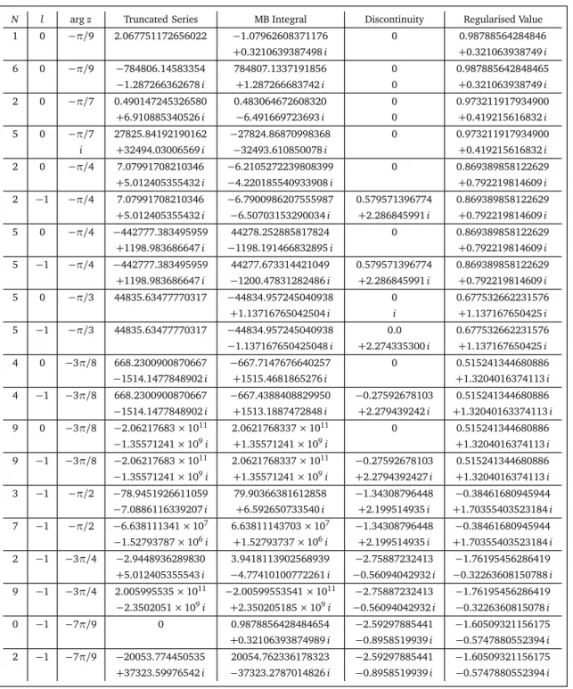
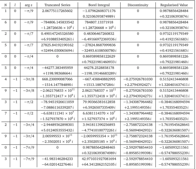
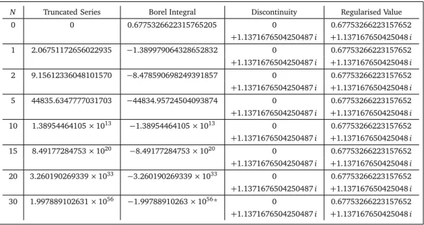
In these resultsN is referred to as the truncation parameter.
Since the limit point is zero in the above series, both types of terminants represent small
zasymptotic series. Had they been expressed in terms of powers of 1/z, which is how Dingle defined them originally in Ref. [8], then they would have represented large z asymptotic series. By asymptotic, we mean here according to the standard Poincar´e prescription discussed on p. 151 of Ref.[33]. As mentioned in the introduction, by adopting this prescription for sufficiently small values of z, namely |z| ≪1, one can truncate the series after only a few terms and still produce an accurate approximation to the actual value of the original function from which the series has been derived. Furthermore, the point at which the approximation begins to break down, known as the optimal point of truncation and denoted by NT in this work, increases or diverges to infinity as z →0. For those seeking an understanding of the important concept of optimal truncation, they should consult Sec. 4.6 of Ref. [24]. As long asN<NT or even forN ≈NT, one can still obtain an accurate approximation to the original function. However, the accuracy of the approximation wanes dramatically as NT → 0, so
that truncation of the series is no longer a valid option for those values of z in either the intermediate region, typically given by 0.1<|z|<2, or for “large values” of|z| greater than 2. As was also discussed in the introduction, since asymptotic series possess limited ranges of applicability and suffer from deficiencies in accuracy, asymptotics as a mathematical discipline has often been ridiculed by pure mathematicians, who point out that mathematics is supposed to be an exact science, not composed of vague concepts and quantities. In reality, the cause for this state of affairs is the adoption of the Poincar´e prescription, particularly truncating asymptotic series.
introduced the integral representation for the gamma function in the numerator, interchanged the order of the summation and integration and finally evaluated the sum. This approach to obtaining limits to divergent series is known more commonly as Borel summation. So let us do the same to the first type of terminant. Then we find that
TI(N,α,z) = Z ∞
0
d t tα−1e−t
∞
X
k=N
(−z t)k . (65)
Now we see that the first type of terminant has been expressed in terms of the geometric series. Therefore, if we introduce the regularised value of the latter series into the above result, then we obtain the regularised value of the first type of terminant. In addition, according to our analysis of the geometric series, it is conditionally convergent for ℜ(−z t)<1. As t ranges from 0 to infinity, this means that the terminant is conditionally convergent forℜz>0 and divergent for all other values ofz. As a consequence, we observe that an asymptotic series need not necessarily be divergent. That is, an asymptotic expansion is not always divergent; it can also be conditionally convergent.
The introduction of the regularised value of the geometric series into Eq. (65) yields
TI(N,α,z)≡(−z)N Z ∞
0
d t t
N+α−1e−t
1+z t . (66)
Since we have already stated that the geometric series is bijective within the principal branch of the complex plane, i.e. for |argz|< π, the regularised value of the first type of terminant given by the above Cauchy integral is also bijective. That is, there is a definite value for each value ofzwithin the principal branch of the complex plane, which means, in turn, that we are moving closer to Euler’s unorthodox view of there being a definite value connected with each divergent series. On the other hand, if in Equivalence (66) we replacez with zexp(−2ilπ), wherel is an arbitrary integer, then we find that
TI(N,α,zexp(−2ilπ))≡(−z)N Z ∞
0
d t t
N+α−1e−t
1+zexp(−2ilπ)t . (67)
We can express the above result as a contour integral in terms of the complex variable s
andC, the line contour along the positive real axis. Then Equivalence (67) becomes
TI(N,α,zexp(−2ilπ))≡(−1)NzN−1 Z
C
ds s
N+α−1e−s
s−(z−1exp((2l−1)iπ)) , (68)
the asymptotic expansion for the complementary error function, which is given as No. 7.1.23 in Ref.[1], is
erfc(z)≡ e −z2
πz
∞
X
k=0
Γ(k+1/2)
(−z2)k , |argz|<3π/4 . (69)
Note that it has been necessary to introduce the equivalence symbol into this result as a consequence of our previous discussion on the properties of an asymptotic series.
According to Equivalence (68) the value of erfc(exp(−3πi/8)) is expected to be equal to erfc(exp(5πi/8)). Yet, the former yields a value of 0.663 282 . . ., while the latter equals 7.117 400 . . .×10−24. Therefore, Equivalence (68) must be restricted to one branch given by either 2lπ <arg(−z2)<(2l+2)π or(l−1/2)π <argz<(l+1/2)π. Then we are left with the problem of deciding whether the equivalence is valid for either −3π/2<argz<−π/2, |argz|<π/2, or forπ/2<argz<3π/2 within the principal branch of the complex plane.
Another problem with Equivalences (66) and (67) is: what do we do when argz =±π? For these values ofzthe Cauchy integral is singular. Whilst this might not be a serious problem with Equivalence (66) where nearly all the principal branch of the complex plane has been covered anyway, for asymptotic expansions written in terms ofzβ, whereβ >1, it will mean that the regularised value will be singular well within inside the principal branch. For exam-ple, in the case of the complementary error function mentioned above, the Cauchy integral is singular along the positive and negative imaginary axes.
These issues can be resolved as a result of a remarkable discovery made in 1857 by Stokes
[31] of what is known today as the Stokes phenomenon. Stokes found that as one moved across specific sectors of the complex plane, called Stokes sectors, asymptotic expansions suddenly acquired extra or jump discontinuous terms. These terms appear at specific rays in the complex plane known as Stokes lines. Along these lines the regularised value as indicated by the Cauchy integral in Equivalence (65) is singular. Moreover, Ch. 1 of Ref.[8]states that the Stokes lines occur at those values of argz, where all the terms in the terminants are of the same sign and homogeneous in phase. For the first type of terminant this means they occur whenever argz= (2k+1)π, where k is an arbitrary integer. Hence, the regularised value given by Equivalence (67) develops extra terms as argzmoves across these lines. In addition, on the lines the Cauchy integral will need to be modified.
It should be emphasised that Stokes sectors and lines are fictitious with regard to the orig-inal function from which an asymptotic expansion is derived. That is, although the asymptotic expansion develops jump discontinuities as the argument of variable in the expansion changes in the complex plane, it does not necessarily mean that the original function is discontinuous. In fact, it is more often than not continuous across the Stokes lines of discontinuity.
valid. This applies to both Stokes sectors and lines. We shall refer to the combination of the series expansion, regularised value and the Stokes sector over which the latter is valid as an asymptotic form.
Frequently, asymptotic expansions are derived when the argument of the variable is real, positive and situated in the principal branch of the complex plane. If this is the case, then we let the primary Stokes sector for Equivalence (67) be given by thel=0 value or in other words, by|argz|<π. Hence, Equivalence (66) as an asymptotic form becomes
TI(N,α,z)≡(−z)N Z ∞
0
d t t
N+α−1e−t
1+z t , |argz|< π . (70)
Let us now turn our attention to the second type of terminant given by Eq. (64). Borel summation of this result yields
TI I(N,α,z)≡zN Z ∞
0
d t t
N+α−1e−t
1−z t . (71)
Ifzis replaced byzexp(−2liπ), wherel is an arbitrary integer integer, then Equivalence (71) becomes
TI I(N,α,zexp(−2ilπ))≡zN Z ∞
0
d t t
N+α−1e−t
1−zexp(−2ilπ)t . (72)
Whilst the integral in the above equivalence is defined for complex values ofz, it is singular for positive real values ofz. This is a problem since it has already been stated that whenever a Type II asymptotic expansion is derived, it is usually for these values ofz.
The situation can be resolved by noting that the Stokes lines for this type of terminant occur at argz=2kπ, where k is an arbitrary integer. Consequently, instead of nominating a primary Stokes sector, we must now nominate a primary Stokes line. Again, this is arbitrary, but we shall take it to be the k=0 line. Furthermore, in accordance with the rules for the Stokes phenomenon given in Ch. 1 of Ref.[8], as soon as argz moves off this line in either direction, the regularised value must acquire jump discontinuous terms. This produces two more problems:
1. Because of the singularity occurring att=1/z , how do we interpret Equivalence (72) along the primary Stokes line?
2. What are the jump discontinuous terms when argz6=0?
Note that these problems apply to the first type of terminant when argzreaches the boundary of the principal branch of the complex plane, i.e. when argz=±π. We shall be able to consider this situation when the Type II situation has been resolved.