A Simple Algorithm for the Restoration of Clipped Speech Signal
Abdelhakim Dahimene, Mohamed Noureddine and Aarab Azrar
Electrical and Electronic Engineering department, Boumerdes University Boumerdes, Algeria, 35000
E-mail: [email protected]
Keywords: speech signal, clipped speech, restoration, interpolation, linear prediction, least square method, Kalman
filter
Received: August 6, 2007
This paper deals with the problem of peak clipped speech. Our basic assumption is that the clipped speech is voiced and can be linearly predicted with a high accuracy. The coefficients of linear prediction are computed using two different algorithms: a least square direct method and a recursive Kalman filter. The speech reconstruction is accomplished using backward prediction.
Povzetek: Predstavljen je algoritem za obnavljanje zvočnega signala.
1
Introduction
Speech acquired by personal computer sound cards is often confronted with two main problems: DC level wandering and peak clipping. While building a data base for our speech recognition project, we have been confronted with both problems. The first one is easily eliminated by simple linear processing but the second one requires more complex algorithms. Peak clipping is fundamentally a non linear distortion. It is characterized by the fact that several successive values of the signal disappear and are replaced by a constant. However, it happens that speech signal is highly predictable. So, in essence, peak clipped speech restoration is a problem of interpolation since we are trying to find missing values by using the properties of the signal itself. There exist several methods of interpolation: polynomial (Lagrange, Newton), spline, etc. In the case of peaked clipped speech, an appropriate method is statistical interpolation [1].
2
Justification of the method
When there is no a priori information on the signal, the classical numerical interpolation methods (polynomial and spline) should be used. Band limited interpolation [2] uses only the fact that the signal is band limited. Statistical interpolation based on linear prediction [2, 4] uses the fact that that speech signal is highly predictable. A speech segment is composed of a sequence of voiced, unvoiced and silence (noise) segments [2]. The type of speech signal that has the greatest probability for being peak clipped is voiced speech [2, 3]. Figure 1 represents a scatter plot of voiced, unvoiced and silence mean magnitude and zero crossing rate of segments of speech. Voiced speech segments are indicated by the letter "V", unvoiced segments by the letter "U" and the silent segments by the letter "S". It shows clearly that the voiced signals cluster at high mean magnitude values.
The mean magnitude is defined as:
( ) ( )
n m
M ∞ x m w n m =−∞
=
∑
− (1)where w(n) is a rectangular window of length 256 samples and the zero crossing rate (ZCR) is:
( ) sgn[ ( )] sgn[ ( 1)] ( )
m
ZCR n +∞ x m x m w n m
=−∞
=
∑
− − − (2)Fortunately, voiced speech happens to be quite predictable. Voiced speech follows quite closely the linear prediction equations [4, 5]. Commercial software like DC-6, from Diamond Cut products, use low order linear prediction for clipped audio signal restoration and the problem of audio signal interpolation have also been addressed by Vaseghi [1] who uses linear prediction from adjacent samples and samples one period away (audio signals are assumed to be periodic).
Voiced speech can be considered as a quasi periodic signal. It can be modelled as the output of a linear time invariant system (during few milliseconds, the system can safely be assumed to be time invariant) driven by a periodic train of impulses. In this case, a quite general formulation of the signal will be:
1 0
p p
n k n k k n k
k k
x a x− b u −
= =
=
∑
+∑
(3)where the signal uk is equal to 1 every T seconds and
zero otherwise, T being the pitch period. akand bkare respectively the recursive and the non recursive parameters of the above production filter of order p. So, within a pitch period (NT samples) and after p samples,
we can write:
1
p n k n k
k
x a x−
=
=
∑
(4)The above equation breaks down in the part of the speech signal that is clipped. So, if we start the time axis at the beginning of a pitch period and if we call NT the
number of samples within the pitch period, we can write:
1
max
;
p
n k n k T
k n
x a x p n N
for x X
− =
= ≤ ≤
<
∑
(5)Xmax being the saturation value.
3
The proposed restoration
algorithm
The proposed algorithm for clipped speech restoration is going to be based on linearly predicting the missing values using equation (4). So, the algorithm consists of two following steps:
- Computation of the prediction coefficients ak. - Linear prediction of the missing values.
3.1
Computation of the prediction
coefficients
The computation of the prediction coefficients ak can be
accomplished either by using a least square solution or by using a recursive algorithm based on Kalman filtering.
For the least square algorithm, we can use equation (5) and build the following matrix vector equation relating speech samples xk:
1 1 1 1 1 2 2 2 1 2 . . . .
. . . (6)
. . . .
. .
T
T T T
p p
p
p p
p
N N N N p p
x x x
x a
x x x
x a
x x x x a
− + + + − − − ⎛ ⎞ ⎛ ⎞ ⎜ ⎟ ⎛ ⎞ ⎜ ⎟ ⎜ ⎟ ⎜ ⎟ ⎜ ⎟ ⎜ ⎟ ⎜ ⎟ ⎜ ⎟= ⎜ ⎟ ⎜ ⎟ ⎜ ⎟ ⎜ ⎟ ⎜ ⎟ ⎜ ⎟ ⎜ ⎟ ⎜ ⎟ ⎜ ⎟ ⎜ ⎟ ⎜ ⎟ ⎜ ⎟ ⎝ ⎠ ⎝ ⎠ ⎝ ⎠
in which all the rows such that xk = Xmaxare deleted. Equation (6) can be written as:
b = X a (7)
and the least square solution of equation (7) can be obtained as [6]:
a = (X XT )−1X bT (8)
Another approach to the evaluation of the prediction coefficient is the following sequential algorithm (Kalman filter) [7, 8] based on the subsequent set of equations and on an autoregressive model. Consider the next state equation:
a(k+1) = a( )k +w( )k
(9) where ( )
(
1, , ,2)
T p k = a a a
a K and w( )k is a white stationary sequence.
The observation model is:
0
1
p
n i n i n
i
x a x − b u
=
=
∑
+ (10)and let us consider C(k− = ⎣1) ⎡xk−1,xk−2, ,L xk p− ⎤⎦ then the observation model becomes:
z k( )=xk =C(k−1) ( )a k +v k( ) (11)
if it is taken that: v k( )=b u0 k
then, starting from an initial estimate
a
ˆ(0)
, we obtain the following recursion:aˆ(k+ =1) aˆ( )k +K(k+1)[xk+1−C( ) ( )]k aˆ k (12)
where Kis the Kalman gain given by:
ˆ 2 0 ˆ ( ) ( ) ( 1) ( ) ( ) ( ) k k k
b k k k
+ = + T a T a V C K
C V C (13)
and the matrix Vaˆ is the variance matrix of the estimator ˆa and is given by the following equation:
Vaˆ(k+ = −1) [I K(k+1) ( )] ( )C k Vaˆ k +Vw (14)
whereVwis the variance matrix of the white noise
process ( )w k .
The algorithm can be initialized by: =σ2
w
V I,
ˆ(0)=
a
V 0 and
b
0=
1
and stopped by using the criterion:aˆ(k+ −1) aˆ( )k 2 ≤
ε
(15)The stopping criterion can also be used for pitch detection because it is evident that the above norm will be large while being in a clipped part, since the autoregressive model will not be valid.
3.2
Interpolation of the missing samples
For the computation of the missing samples, equation (4) can be used starting from p previous samples. This interpolation is referred to as forward. The missing samples can also be predicted from p samples that follow the missing part. The first sample can be obtained by solving equation (4) as:
1
; 1
p
n p i n p i T
i
x−
α
x − + p n N=
=
∑
+ ≤ ≤ (16)where the coefficients αi are computed from the
coefficients ai using:
1 1 1 1 1 ; ; ; p p p
p p p
a a
a a a
α
−α
α
−
Consequently, the reconstruction is done using backward interpolation.
4
Results
In order to test the previously defined algorithms, we are going to use synthetic and natural speech. The natural speech comes from a very large database of speech samples that were collected for the construction of a speech recognition system in colloquial Algerian Arabic [9]. The pitch frequency is about 100 Hz for male speaker and about 220 Hz for a female one. This corresponds to a pitch period T being between 4.5 ms to 10 ms. So, if a reliable estimation of the prediction parameters is desired, we need a fairly high sampling frequency. For example, a sampling frequency of 10 kHz (sampling period of 100 µs) will provide between 45 and 100 samples for a pitch period. A sampling frequency of 44.1 kHz (sampling period of 22.73 µs) is chosen, which provides between 198 and 440 samples for a pitch period, which is quite reasonable. Also, in all of the following tests, the speech signal is normalized to a maximum value of one.
4.1
Synthetic speech
First the algorithm is tested with a synthetic vowel. The choice of synthetic speech is motivated by the fact that it follows exactly the linear prediction model. The vowel /a/ is generated using the following formants [5]:
- The frequencies ( )Fi and the bandwidths (BWi)necessary to specify each formant are shown in the following table.
Formant
F Hz
i(
)
BW Hz
i(
)
1 730 60 2 1090 100 3 2440 120 4 3500 175 5 4500 281 Table 1: Formant Frequencies and Bandwidths [5] - The pitch frequency is 120 Hz (male speaker), which corresponds to NT = 367 samples. Figure 2 shows few
periods of the synthetic vowel /a/. The prediction order is set to p = 10.
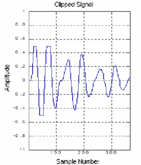
This signal is clipped to a level of ±0.5 and restored using both methods (least square and Kalman filter method).
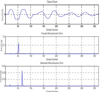
Figure 3 shows one pitch period of the clipped signal. A window of at least 75 samples following the clipped region is used to compute the predictor coefficients.
0 500 1000 1500 2000 2500 3000 3500
-1 -0.8 -0.6 -0.4 -0.2 0 0.2 0.4 0.6 0.8 1
Sample Number
A
m
pl
itude
Figure 2 : Synthetic Vowel /a/ Normalized Amplitude Waveform
Figure 3 : Clipped artificial vowel
50 100 150 200 250 300 350 -1
0
1 Clipped Signal
Sample Number
A
m
plit
ud
e
50 100 150 200 250 300 350
0 0.01 0.02 0.03
Sample Number
A
m
plit
ud
e
Backward Reconstruction Error
50 100 150 200 250 300 350
0 0.1 0.2
Sample Number
A
m
plit
ud
e
Forward Reconstruction Error
Figure 4 : Forward and Backward Reconstruction Error for Synthetic Speech
Kalman filter is also used for the estimation of the prediction parameters. The stopping criterion of the recursive Kalman algorithm is defined as:
2
( 1) ( )
a k+ −a k <ε, where ε is a small positive number that describes the convergence of the algorithm. From the plot of a k( + −1) a k( ) 2 over 04 pitch periods of the signal (under:σ =0.1and b0 =1) shown in figure 5, it appears that the value
ε
=0.00008 is acceptable.
200 400 600 800 1000 1200 1400 -1
-0.5 0 0.5 1
Sample Number
A
m
pl
iy
ude
Clipped Speech Signal
200 400 600 800 1000 1200 1400 0
0.02 0.04 0.06 0.08 0.1
X: 93 Y: 8.137e-005
Sample Number
Am
plit
ud
e
Converge Criterion
Figure 5 : Kalman Filter Convergence Criterion Plot As stated before, the above convergence criterion ( a k( + −1) a k( )2) can be used for pitch detection. This is well illustrated in figure 5, the large values occurs at the clipped parts generally located at the beginning of the pitch period. After several tests, the following initial values:σ =0.1 , b0 =1, (0)aˆ =0have been selected. After estimation of the prediction parameters and backward prediction, the error is drawn in figure 6.
0 50 100 150 200 250 300 350 400
0 0.05 0.1 0.15 0.2 0.25
Sample Number
Am
pl
itu
de
Figure 6 : Kalman Filter Error signal waveform
We observe that the error using the Kalman filter estimation is much larger that the one using the least square method. Another problem that is encountered is the large computation time. So, in the following tests, the results obtained by the least square method are the only ones that will be presented.
4.2
Artificially clipped natural speech
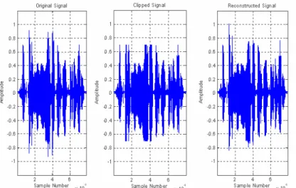
After being applied on a synthetic speech, the proposed technique of interpolation (least square evaluation of the parameters and backward reconstruction) is applied on a voluntarily clipped natural speech. The unclipped signal is taken as a reference when evaluating the reconstruction process precision.
The used recorded speech signal consists on numbers pronounced in Algerian Arabic, sampled at 16 KHz, taken from the database [9]. An audio processing software (Cool Edit Pro 2.1 from Syntrillium Software Corporation) is used to adjust the sampling frequency to 44.1 KHz.
1 2 3 4 5 6 7 8 x 10⁴ -1
-0.5 0 0.5 1
Sample Number
A
m
pl
itude
Reconstructed Signal
1 2 3 4 5 6 7 8
x 104 0
0.05 0.1 0.15 0.2
Sample Number
A
m
plit
ud
e
Reconstruction Error
Figure 8 : Artificially Clipped Natural Speech Reconstruction Error
4.3
Clipped natural speech
The final test is performed on clipped natural speech. Figures 9 and 10 show the clipped and the reconstructed signal. It is impossible in this case to present an error plot due to the absence of the original unclipped signal. The only comment that can be made about the above plots is that the reconstructed signal looks like an unclipped signal. Since there is no reference to objectively evaluate the performance of the algorithm, a subjective criterion is used for judging the quality of the restoration. The speech samples (clipped and restored) were presented to several listeners and they were asked to evaluate the intelligibility of the message by giving a grade between zero and five (zero meaning completely unintelligible and five meaning very clear). The result is a great improvement in intelligibility. The clipped signal was given an average grade of about two while the restored signal received a grade that varied between four and five.
Figure 9 : Clipped Natural Speech Backward Reconstruction using Least Square Estimation
Figure 10 : Zoomed segment of the reconstruction process.
4.4
Discussion
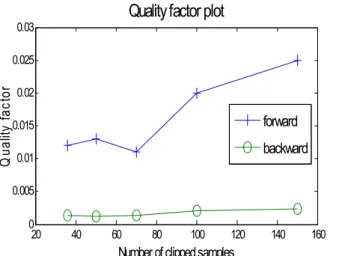
It is quite hard to provide a figure of merit for the method other than the plot of the error signal between the unclipped and the reconstructed speech signal. We can observe from the plots in figure 4 and 8 that two parameters determine the quality of the reconstruction: the amplitude and the duration of the error spikes. We can resume both parameters in the following quality factor:
1 1 Nc ( )
k c
e k
N =
Γ =
∑
(18)where e(k) is the error signal between the unclipped and the reconstructed speech signal and Nc is the number
of clipped samples. Figure 11 shows the quality factor for forward and backward reconstruction as a function of the number of clipped samples per pitch period for synthetic speech. For clipped natural speech, it of course impossible to provide such data. For artificially clipped natural speech, the quality factor curve using backward reconstruction is so close to the one for forward reconstruction for synthetic speech that it is impossible to provide a separate plot. From the different plots (figure 4, 8 and 11), we can conclude that the estimation of parameters using least square followed by a backward reconstruction offers the best results in term of accuracy.
20 40 60 80 100 120 140 160 0
0.005 0.01 0.015 0.02 0.025 0.03
Number of clipped samples
Q
ual
ity
fa
ct
or
Quality factor plot
forward backward
Figure 11 : Plot of quality factor vs. number of clipped samples for synthetic speech.
5
Conclusion
In this paper, an algorithm for clipped speech restoration using linear prediction has been presented and tested. It is able to restore completely the clipped speech. Two different methods for estimating the prediction parameters have been tested. The first one consists on block least square estimation while the second one is a recursive method. It appears that the recursive method is
pitch synchronous but quite inefficient while the block least square is very efficient and very precise. The block least square method followed by backward prediction has been implemented as part of a larger program for speech pre-processing in view of recognition and the results are a great improvement in the recognition rate.
6
References
[1] Vaseghi, S.V., “Advanced Signal Processing and Digital Noise Reduction”, John Wiley and
Teubneur 1996.
[2] Rabiner, L. R., Shafer, R. W., “Digital Processing of Speech Signals”, Prentice Hall, New Jersey, 1978.
[3] Brakta, N. and Hadibi, M., “Pattern Recognition Techniques Applied to Speech Recognition”, Final Year Project, INELEC, 1999.
[4] Makhoul, J., "Linear Prediction, A Tutorial Review", Proceeding of the IEEE, (63), pp. 561-580, April 1976.
[5] Chandra, S. and Lin, W. C., "Experimental Comparison between Stationary and Non Stationary Formulations of Linear Prediction Applied to Voiced Speech Analysis", IEEE trans. of ASSP, (22)6, Dec. 1974.
[6] Lawson, C.L., and Hanson R.J., “Solving Least Squares Problems”, Prentice Hall, 1974.
[7] Srinath, M.,D. and Rajasekaran, P., K., “An Introduction to Statistical Signal Processing with Applications”, John Wiley & Sons, 1979.
[8] Gueguen, C., J., and Carayannis, G., "Analyse de la Parole par Filtrage Optimal de Kalman", Automatisme, Tome XVIII, March 1973, pp.99-105.
![Figure 1: Mean magnitude and ZCR scatter plot [3]](https://thumb-us.123doks.com/thumbv2/123dok_us/8046096.2130562/1.892.469.803.509.814/figure-mean-magnitude-zcr-scatter-plot.webp)