Consensus From Proof-of-Work Puzzles

(1)

Consensus From Proof-of-Work Puzzles

Patrik Keller

Master Thesis 2018

(2)

Abstract

In this thesis we analyze the role of puzzles in blockchain based distributed systems. We extract the relevant properties from existing puzzle mechanisms and use them to define an abstract notion for proof-of-work puzzles. The resulting puzzles have exponentially distributed solving time and allow to consider nodes and parties with individual solving capabilities. We use the new definition of proof-of-work puzzles in a bottom-up construction of a blockchain protocol. Our new model is compatible with the Bitcoin backbone protocol [16], in the sense that we can transfer the backbone protocol’s properties to our model. During the construction we try to pinpoint the original design decisions made for Bitcoin [25].

This thesis was written for the master program in computer science at the University of Innsbruck. The supervisor was Univ.-Prof. Dr. Rainer Böhme.

(3)

1 Introduction

In 2008, Nakamoto [25] published Bitcoin, the first cryptographic currency based on a so-called blockchain protocol. The protocol allows its participants to maintain a distributed ledger, i. e. a consistent, publicly readable data structure with controlled, append-only write access. Bitcoin uses such a ledger to record transactions between Bitcoin addresses. The system listens for clients’ transaction requests, orders them and builds a valid and globally consistent series of transactions. This history of transactions allows to reconstruct the actual balances of each address.

The major novelty introduced with Bitcoin and the blockchain protocol is that nodes can join and leave the distributed system at any time. The protocol does not rely on any kind of identification of the nodes. Instead it uses a mechanism known as proof-of-work to restrict write access to the ledger. Each node orders the incoming transactions locally and writes them into a block. Each block references a preceding block. The blocks build a chain. Completed blocks are send to the other nodes, which always try to extend the longest chain they are aware of. The protocol avoids the broadcast of conflicting blocks by ensuring that block creation takes a substantial and highly indeterministic amount of time. For that purpose, the completion of each block requires to solve a unique computational puzzle.

In proof-of-work blockchain protocols, the puzzle is typically based on cryptographic hash functions. The puzzle for a block is solved by finding a short hash for this block as input. By short hash we mean, that the hash interpreted as number must be smaller than a certain bound set by the protocol. The block contains a field that can be chosen freely by the solving node. This allows to solve the puzzle by repeatedly applying the deterministic hash function on changing inputs until a short hash is found.

The puzzle mechanism enforces a rate limit on extending the ledger. Each write requires to spend computational resources on a unique puzzle. Blocks are chained together, such that changing one block invalidates all successors. Honest nodes accept the longest chain of blocks as true history. A rewrite of a historic block thus requires an adversary to find new solutions for all subsequent blocks. Since each solution requires significant computational effort, rewriting the history becomes unachievable over time.

The mechanism relies on honest participation. If honest parties would provide no or only a few puzzle solutions, an adversary could influence the protocol execution by simply solving puzzles faster. In order to make manipulation harder for adversaries, the system motivates all participants to provide solutions. It gives rewards for each found solution. The puzzle solving process constitutes a lottery, where buying tickets corresponds to solving attempts and winning to actually finding a solution. In the context of doing computational work for occasional rewards, puzzle solving is often called mining. Participants in the protocol are called miners.

(5)

The reward system is based on a cryptographic currency that is implemented on top of the blockchain protocol. Identities can hold amounts of a digital currency. The currency is scarce since new units can only be created by solving puzzles. The currency is liquid because units can be transferred between identities. Scarcity and liquidity make the cryptographic currency resemble true money.

1.1 Byzantine Fault Tolerance

Distributed systems are traditionally modelled as a set of nodes that interact over the network with the goal of jointly providing a service to its clients [31]. Clients may connect to a subset of the nodes for consuming the service. Nodes synchronize their states with the other nodes by communicating over a network as specified by a protocol.

The protocol specifies how nodes should interact, but obviously, an adversary may choose to deviate from the specification. Hence, protocols are analysed with respect to how many deviating nodes they can tolerate without an interruption of the service. Adversarial behaviour is modelled by allowing arbitrary or so-called Byzantine faults [22]. Failing nodes may deviate from the protocol in any way. This includes collaboration between faulty nodes and worst-case behaviour of the adversary which might be unknown at the time of the protocol analysis.

Protocols that can stay operational in the presence of Byzantine faults are called Byzantine fault tolerant (BFT). Usually, Byzantine fault tolerance can only be proven under strong assumptions. These assumptions often include an upper bound on the number of faulty nodes and some sort of reliability of the network that the nodes use for communication.

A typical set of properties are consistency, availability and partition tolerance [31]. A system is consistent if all honest nodes agree on the current state of the service. A system is available if it is operational and processing incoming requests by clients. A system is partition tolerant if it is able to maintain consistency and availability, even if the there is a strict subset of the honest nodes that cannot communicate with the rest.

Unfortunately, a Byzantine fault tolerant system with these properties cannot exist without assumptions on the communication model. If messages can be delayed forever, the properties are conflicting.

Assume that the nodes are divided into two subsets A and B. Nodes in B cannot communicate with nodes inA and vice versa. A node in Areceives a request by a client and has to update its local state. Availability implies, that the state update is processed. Consistency and partition tolerance imply that all nodes agree on the same updated state. But this violates the assumption, that no messages can be exchanged between A

andB. Gilbert and Lynch [17] provide a proof for the CAP-theorem, which extends this statement by the fact, that any two of the three properties can be satisfied.

Obviously any two out of the properties, are not sufficient to build useful distributed systems. Consistency and availability are vital and partitions cannot be ruled out completely. Hence security analyses typically assume that messages will eventually be delivered. In the partially asynchronous setting, where messages are guaranteed to be delivered after some delay, Byzantine fault tolerant protocols are possible. Prominent

(6)

examples are Paxos by Lamport [21] and the practical Byzantine fault tolerant (PBFT) protocol by Castro and Liskov [8]. Both make no a-priori assumption on the message delay and guarantee availability and consistency after messages are eventually delivered.

Also blockchain protocols can be analysed in the Byzantine framework. For that purpose, Garay et al. [16] formulate an abstract version of the Bitcoin protocol. Their so-called Bitcoin backbone protocol is executed in discrete rounds. Every honest node has one puzzle solving attempt per round. The probability of finding a solution at a given round is constant and the same for all nodes. An adversary who controls nnodes is allowed to maken solving attempts at the end the round. Messages are assumed to be delivered at the end of each round [16] or within a known upper bound of rounds [28].

In this model, the backbone protocol guarantees consistency, growth, and chain-quality. In this context, consistency means that all but the most recent blocks are consistent between all nodes, chain-growth means that the blockchain grows steadily, and chain-quality implies that blocks of honest nodes are added regularly to the chain. For the cryptographic currency implemented on top of the backbone protocol, these three properties imply persistence and liveness, i. e. client transactions are processed and then persistently recorded into the distributed blockchain.

1.2 Motivation and Scope

A major limitation of the classical Byzantine fault tolerance framework is that it assumes a limited fraction of dishonest nodes. The protocols fail if an adversary is able to impersonate honest nodes or add new nodes to the network. In order to mitigate such so-called Sybil attacks, Byzantine fault tolerant system have to rely on a centrally managed identification system [10]. We say that BFT protocols require strong identities.

Contrarily, blockchain systems like Bitcoin are open for participation. Nodes can be added and removed from the network at any time. Nodes have no identity and the protocol does not rely on such. The only thing that matters, is how much puzzles a party can solve per time – how the solutions are spread over different nodes is not important.

In order to analyze blockchain protocols in the BFT framework, Garay et al. [16] and Pass et al. [28] have to rely on counterintuitive assumptions. Namely, they assume a fixed number of nodes with equal puzzle solving capabilities. In practice, we observe a changing number of nodes with changing individual puzzle solving rates. The security properties of a blockchain protocol are intuitively related to the adversaries share of the overall solving power. Instead of analysing, how many Byzantine nodes can be tolerated, one has to consider how many of the puzzle solutions are found by Byzantine nodes. In this thesis, we propose a framework, that allows such considerations. We will define proof-of-work puzzles that enable to measure the solving power of nodes and parties in an interoperable way. This allows to abstract from the amount of nodes and measure the adversaries solving power relative to the combined solving power of all honest nodes. Security properties of blockchain protocols can then be restated with respect to the adversaries share in solving power.

(7)

All proof-of-work based blockchain implementations that we are aware off, use puzzle based on cryptographic hash functions or a variation thereof. The concept is always the same: puzzle solutions are hashes with certain rare properties. In order to find a solution, the hash function has to be evaluated repeatedly on changing inputs. In this thesis, we extract the relevant properties of such puzzles and use them to define abstract requirements for proof-of-work puzzles. Thereby, we hope to provide insights into the puzzle mechanism and enable research on a wider range of puzzles.

Starting from the core concept of puzzles, we construct a complete blockchain protocol. It will be compatible with the security analyses made in the BFT framework [16, 28] in the sense that their results can be transferred to our new model. It will also be intuitive, i. e. it will reflect the openness of blockchain protocols and the varying solving rates of different parties and nodes.

During this bottom-up construction, we try to separately highlight the original design decisions made for Bitcoin [25]. We hope to provide insight into the different building blocks of blockchain protocols and how they depend on each other.

1.3 Layout of the Thesis

We start by recalling necessary basic principles in the preliminary section 2. The section includes a short recapitulation of some relevant probability distributions in section 2.1. We will state their basic properties and show how the distributions depend each other. In section 2.2, we recall the notion of random oracles. They allow us to theoretically model ideal, cryptographic hash functions.

We make a first contribution in section 3, where we define abstract puzzles for proof-of-work based on the probability theory given in section 2.1. Puzzles are functions that map payloads to puzzle instances. Puzzle instances are trivially to evaluate solution verifiers. Solutions will be verified on each node, but nodes cannot observe how solutions where found. The solving mechanism is naturally target of optimizations. Nodes do not solve the puzzles at the same rate, but we assume that proof-of-work puzzles have exponentially distributed solving time, instances are equally hard to solve for all payloads, and their hardness can be adjusted via an external parameter. We will provide an exemplary puzzle based on the random oracle model from section 2.2.

Based on the proof-of-work puzzles, we describe a small toy protocol in section 4. It allows the nodes of a distributed system to elect one out of many proposed values. For that purpose, the nodes accumulate and share votes. A vote for a value is a solution for a puzzle with this value as part of the payload. Hence, voting requires to solve puzzle instances.

Honest nodes start with voting for their own proposed values. As soon as they receive valid votes from other nodes, the nodes always adopt the value with the most votes. As soon as a predefined number of votes is found, the protocol terminates.

This toy protocol contains the core principles that we need for the construction of a proceeding consensus protocol in section 5. Instead of terminating after a fixed amount of votes, participants collectively write an ongoing history of elected values. Puzzle payloads

(8)

are now lists of values. With each vote, the list is extended by one value. A vote on a list confirms all of its prefixes. Disputes on the inclusion and order of values are settled over time, because honest nodes always extend the longest available history.

The proceeding consensus protocol resembles the Bitcoin backbone protocol [16], where the random oracle puzzle is replaced with our abstract puzzle mechanism. We use section 5 to demonstrate compatibility with existing work [16, 28] by restating the backbone protocol’s security properties in our model.

In section 6, we show how actual applications can be implemented on top of the abstract protocol for proceeding consensus. Section 6.1 describes, how the growing list of values can be used to implement general distributed state machines [20, 30]. Unfortunately, using this method directly on the protocol for proceeding consensus causes severe performance and scalability issues.

On the one hand, each state update requires to solve a puzzle, that is designed to take a considerable amount of time. This naturally causes low throughput. In section 6.3, we discuss how the throughput can be increased by bundling multiple state updates in blocks of events that are recorded as a single value.

On the other hand, the proceeding consensus protocol from section 5 requires the retransmission of the complete history of values with each found puzzle solution. This causes the message size to grow linearly over time and effectively renders the protocol unusable. In section 6.2, we describe how hash-linked lists allow to make message size constant.

In section 7 we conclude with a discussion of our work, its relation to others work and the overall state of research.

(9)

2 Preliminaries

This section gives some of the background information that is necessary for understanding the thesis. We start by defining our mathematical notation. Then, we recall basic probability distributions together with some of their relevant properties. At last, we briefly describe the random oracle model, which allows us to argue about applications of cryptographic hash functions.

Notation

B The binary set, i. e.B={⊥,>}={0,1}.

N The natural numbers, starting from1. We use N0 to explicitly include the0. [a, b] The integer interval fromato b, i. e. [a, b] ={n∈N:a≤n≤b}.

|S| The cardinality of set S.

H(·) The random oracle as defined in section 2.2 or a approximation thereof.

P(S) The powerset ofS, i. e. P(S) ={s⊂S}.

x∼X The random variable x is drawn from distribution X. Within algorithms,

x∼X stands for assigning a fresh and independent instantiation of a random variablev ∼X to the variablex.

Pr

·

For an event x,Pr x

denotes the probability ofx being true. E·

For a random variablex,Exdenotes the expected value of x.

2.1 Primer on Probability Distributions

In this preliminary section, we recap some probability distributions and their basic properties. Detailed background information can be found in introductory textbooks on probability theory as for example [18].

We start with the uniform distribution. It can have continuous or discrete support. Its key property is, that each element of the support is equally likely to be observed. This implies that the probability mass functions or the probability density function respectively, are constant. A uniform distribution is fully defined by specifying its support. For a uniformly distributed random variable X0 with support S, we writeX0 ∼U nif(S). For

the discrete and finite case, we get the following probability mass function.

PrX0=x

= 1

|S|

Whenever it is clear from the context, thatS is a set, we write· ∼S to abbreviate· ∼

(10)

The Bernoulli distribution has supportB. A Bernoulli distributed random variable can either instantiate to⊥ or>. The distribution is parametrized by a single parameter p. The outcomes > and⊥ are often interpreted as success and failure. The parameter p

is then called success probability. The probability mass function of a random variable

X0 ∼Bern(p)is Pr x=X0 = ( p if x=> 1−p if x=⊥ .

Imagine an experiment, whereX0 is iteratively instantiated. The number of Bernoulli

trials until the first success is observed, is again a random variable. LetX1 denote such a

random variable. ThenX1 is geometrically distributed. We write X1∼Geom(p). The

specification yields the probability mass function

Prk=X1

= (1−p)k−1·p for k∈N.

The expected value of X1 is p−1.

Geometrically distributed random variables can be interpreted on a continuous time scale by assigning a fixed time step sto each Bernoulli trial. The success probability p

can then be restated as number of expected successes per time. This new parameter

λ=p/sis called rate. Now, we can observe the random time s·X1 until the first success

is observed.

For small time stepsand success probabilityp, the random times·X1is approximately

exponentially distributed. In fact, when making s infinitely small while maintaining constant rateλby setting p=λ·s, then the resulting random variable is exponentially distributed with rate λ. AssumeX2,s/s∼Geom(λ·s) and X2 ∼Exp(λ), then

lim

s→0X2,s =X2 .

The exponential distribution has the following probability density and cumulative distribution functions. fX2(x) = ( λe−λx if x≥0 0 else PrX2 ≤x = ( 1−λe−λx if x≥0 0 else

An exponentially distributed variable has expected value E X2 =λ−1 and variance X2 =λ−2. Further,X2 is memoryless, i. e. ∀s, t >0 :PrX2> s+t |X2 > s =PrX2 > t .

The minimum of multiple independent exponentially distributed variables is of partic-ular interest for our thesis. It allows to model the time until first success when observing multiple independent Bernoulli experiments in parallel. Interestingly, the minimum

(11)

is again exponentially distributed. Consider npairwise independent random variables

Yi ∼Exp(λi) for i∈[1, n]and letλ=λ1+· · ·+λn, then

min{Yi} ∼Exp(λ) .

Besides the first success, we can also wait for and observe the time until thek-th success. Since all instantiations of the Bernoulli variable are independent the time between the

(k−1)-th success and k-th success in equally distributed like the time until the first success. Thus the time until the k-th success can be modelled as sum of independent random variables that are identically, exponentially distributed.

Let Z1, . . . , Zk ∼Exp(λ) be independent. LetX3 =Pk_i₌₁Zi. Then, X3 is Gamma

distributed with shape parameterk and rate parameterλ. We write X3∼Gamma(k, λ)

and get the following probability density function.

fX3(x) =

(_λk_xk−1_e−λx

(k−1)! if x≥0

0 else

The expected value is EX3

=k·λ−1 and the variance X2 =k·λ−2.

2.2 Random Oracle

Applications of cryptographic hash functions are usually modelled in the random oracle model [4, 6]. Loosely spoken, the random oracleH resembles an idealized hash function. It is globally available and can be called by any node at any time. His a function that maps bit strings of arbitrary length to outputs of fixed length, i. e.

H:B∗→Bl ,

wherel is the security parameter. For any input, the corresponding output is uniformly and independently drawn formBl. Repeated queries with the same input return the same output. Algorithm 1 shows a schematic representation ofH. Clients can invoke H(·), but have no direct access to the memorized values inS.

Algorithm 1Schematic representation of the random oracle

Return values are drawn uniformly fromBl and persisted inS for later queries on the same input. 1: functionH(x) 2: if x6∈S then 3: r ∼Bl 4: S[x]←r 5: returnS[x]

Two core properties follow. Assuming no prior knowledge andx∈B∗, thenH(x)∼Bl. If additionallyy∈B∗ andy6=x, thenH(x) andH(y) are independent.

(12)

Applications often rely on properties that follow for l ≥256. Amongst others, the such a random oracleHis

• preimage resistant, meaning that given a valueh∈Bl, it is effectively impossible to find ax∈B∗ such thatH(x) =h,

• second preimage resistant, i. e. given x ∈B∗ it is effectively impossible to find a

y∈B∗ such thatH(y) =H(x) and y6=x, and

• collision resistant, i. e. it is effectively impossible to find any x, y∈B∗, such that

H(x) =H(y)and y6=x.

Algorithm 1 cannot be implemented in practice without exposing the memorized values. Cryptographic hash functions are functions that are good practical approximations of the random oracle. With ongoing research, growing computational power, and algorithmic advance cryptographic hash function tend to become less secure over time. Protocols that are proven secure in the random oracle model, have to be revised regularly with respect to how they use cryptographic hash functions and whether the hash functions are still secure in their context.

Throughout the thesis, we take the following notational shortcut. While the random oracle is defined on bit sequences, we will regularly use it on arbitrary types of inputs and integer output. For inputs we assume that they are implicitly encoded in binary format. Whenever the output is interpreted as integer, we assume thatBl is decoded to numbers in[0,2l−1].

(13)

3 Abstract Puzzles as Proof-of-Work

Our major contribution is the definition of abstract puzzles that can be used in construc-tions of proof-of-work based blockchain protocols.

The puzzles are inspired by work of Dwork and Naor [12], who introduced so-called cost functions for combating junk email in 1992. Their main idea was to require email clients to solve a computational task for each message they send. The proposed cost-functions have backdoors that allow mail operators to send bulk messages, while creators of junk email suffer from high costs imposed by the solving the computational tasks.

A practical cost-function was proposed by Back [1] in 1997 and implemented in the spam mitigation protocol Hashcash. The computational task does not have any backdoor for mail operators. In fact, it constitutes a puzzle in our sense. It was later used in the implementation of Bitcoin [25] and other proof-of-work based blockchains. The puzzle will serve as example later in this section.

The Hashcash puzzle relies on the partial inversion resistance of cryptographic hash functions. It is thus analysed in the random oracle model. An earlier attempt to abstract from the exact puzzle and the random oracle model was made by Miller et al. [24]. Their Scratch-Off puzzles capture the necessary properties of the Hashcash puzzle, but their definition is based on rounds and analysed in discrete time.

Our abstract puzzles work in continuous time and do not rely on the random oracle model. Additionally, they allow to measure the solving power of nodes, parties and the complete network. These properties simplify the analysis in Byzantine and game-theoretical models.

The puzzles are defined as generator functions that map elements of the set of payloadsD to puzzle instances. Each puzzle instance is a search task. It is specified by a subset of the candidate setC. All elements of this subset are solutions to the puzzle instance.

For our application, we need puzzle solution verification to be easy. Further, puzzles should have at least one solution. Puzzles are solved using probabilistic algorithms. Finding solutions should be moderately hard, i. e. the expected time to solve puzzle instances should be controllable by changing an additional parameter to the generating function.

Definition 1(Puzzle). A tuple(D,C, P)is called a puzzle onDif the following conditions are true:

1. P is a function that maps elements of Dto subsets of C, i. e.

P :D →P(C) .

2. Puzzle solution verification is easy, i. e. there exists a polynomial time algorithm Verif on inputd∈ D andc∈ C, such that

(14)

3. All puzzle instances have solutions, i. e.

∀ d∈ D:|P(d)|>0 .

We refer to Das the set of payloads and Cas the set of solution candidates. P(d) is called a puzzle instance or solution set. _Verif is the verification algorithm for puzzle

(D,C, P). Often when D and C can be derived from the context, we simply write P

instead of (D,C, P).

The algorithm for puzzle solving is intentionally kept out of the above definition. Puzzle solving is part of a competition and participating parties will try to replace the algorithm with the most efficient version available. Solving algorithms search through the set of candidates and return a puzzle solution. The search algorithm might be probabilistic.

Definition 2 (Solving Algorithm). A probabilistic algorithm_Solve, that takes as input an arbitrary payloadd∈ D, is called asolving algorithmfor puzzleP if it returns solutions for instances ofP, i. e.

∀d∈ D:Solve (d)∈P(d) .

The random variabletime_Solve,M(d)denotes the running time until algorithmSolve terminates on input dand machineM. In most cases, we argue on the distribution of time_Solve,M(d). If the exact machine is not of particular interest, we writetimeSolve(d)

and assume an arbitrary but fixed machineM.

A solving algorithm_Aiscompetitive for puzzle(D,C, P)if for any solving algorithm_B and d∈ D

Etime_A(d)<=EtimeB(d)

.

Whenever the exact competitive solving algorithm does not matter, we write time(d)

and assume an arbitrary but fixed competitive solving algorithm.

Every puzzle instance P(d) can be solved using the trivial solving algorithm Triv-Solvethat iteratively draws a candidate cfrom C uniformly untilVerif (d, c) returns true. Algorithm 2 provides a listing of this algorithm.

Algorithm 2Trivial solving algorithm for puzzle(D,C, P)

Solves puzzle instance generated from payloadd∈ D by trial and error.

1: function_TrivSolve(d)

2: repeat

3: c∼ C

4: until_Verif (d, c)

5: returnc

The trivial solving algorithm terminates almost surely, i. e. the probability that the algorithm terminates equals one. SinceP(d)is non-empty according to the definition of a puzzle, the probability that _Verif returns true is strictly greater than zero on each

(15)

iteration. The probability that the algorithm runs more than n iterations decreases exponentially inn. More formally:

PrVerif (d, c) =>=Prc∈P(d)= |P_|C|(d)| >0

And thus, with the random variableXdenoting the number of iterations until_TrivSolve terminates: Pr X > n = 1−|P(d)| |C| n −→0

Thereby _TrivSolveterminates almost surely. Additionally, one can see that X is geometrically distributed with success probability |P_|C|(d)|.

For practicable puzzles,_Verifterminates quickly and there are relatively few solutions (|P(d)| |C|). Iterations happen at a fast rate but with a very small success

proba-bility. The waiting time for finding a solution using_TrivSolve is then approximately exponentially distributed (see section 2.1).

We note that the form of the distribution is independent of the actual machine used for solving. Only the rate parameter of the exponential distribution changes from machine to machine. The higher the number of iterations a machine can handle per fixed time unit, the higher its rate parameter.

Next, we consider a parallel version of _TrivSolve. A party launches ninstances of TrivSolve. Let the random variablesX1, . . . , Xn denote the time until termination of these instances. Then there existλ1, . . . , λn such that

Xi

appr.

∼ Exp(λi) . (1)

Candidates are drawn independently between both iterations and instances. Thus

X1, . . . , Xn are independent and the minimal solving time is again exponentially dis-tributed with

min{Xi}

appr.

∼ Exp(λ1+· · ·+λn) . (2)

This argument can be extended to multiple parties that compete for finding the solution first. Assume there arem parties, each trying to solve the puzzle starting at the same time. Each party might use multiple instances of the solving algorithm in parallel. Following the previous argument, the time until a party finds its first solutions is exponentially distributed. Let Y1, . . . , Ym denote the random times until the j-th party finds its first solution. Then there exist λ0₁, . . . , λ0_m such that

Yj

appr.

∼ Exp(λ0_j) . (3)

As before, the time until the first party finds a solution is exponentially distributed with rateλ0₁+· · ·+λ0_m. Additionally, the probability of finding the first solution is weighted by the parties solving rates, i. e.

Prj-th party wins=Pr∀k∈[1, m] :Yj ≤Yk appr. = λ 0 j Pm k=1λ0k . (4)

(16)

The last property demonstrates some sort of fairness of the competition for the first solution. If all parties have the same solving rate, their winning probabilities are equal. A party that doubles its rate also doubles its odds of winning. It allows to build a basic lottery, where the odds of winning are bound to the participants share of overall computational effort put into solving the puzzle. In the remainder of the thesis, we will rely on this property for building distributed consensus protocols.

Motivated by the above observations, we define exponential and regular puzzles, a unit for measuring solving power on such puzzles, and moderately hard families of puzzles. For such puzzles, the approximations 1 to 4 turn into equalities. This makes the puzzles convenient for the analysis in later sections.

Definition 3 (Exponential Puzzle). A puzzle (D,C, P) is exponential, if all competitive algorithms for finding solutions have exponentially distributed solving time. Formally, for any competitive solving algorithm_Solve and input d∈ D there existsλ >0 such that time_Solve(d)∼Exp(λ).

Definition 4(Regularity). A puzzle(D,C, P)is calledregular, if the choice of the payload does not affect the expected solving time of competitive algorithms. More formal, the puzzle (D,C, P) is regular if there exists a constantc∈_R+₀, such that

∀ d∈ D:Etime(d)=c .

For exponential puzzles, regularity implies constant solving rate λ= 1/c. For regular puzzles we abbreviatetime(d) withtime, since dhas no effect.

Definition 5 (Solving Power). For a fixed puzzle (D,C, P), the solving times of both machines and parties, that parallelize search on multiple machines, are exponentially distributed. Forth on, we call the rate parameter to these exponential distributions solving power. By saying that machineA has solving powerλA, we mean

timeA∼Exp(λa) .

For a party, that operates a set S of machines with solving powers {λs}s∈S, we say that the party has solving power

λ=X

s∈S λs .

Definition 6 (Moderate Hardness). A family{(D,C, Pγ)}γ∈Γ of regular and exponential

puzzles is calledmoderately hard if for any target timetthere exists a difficulty parameter

γ ∈Γ, such thatEtime=t.

A network consisting of machines M1, . . . , Mn with solving powers λ1, . . . , λnis said to be moderated at rateλif γ ∈Γ is chosen such that

λ1+· · ·+λn=λ .

If all of these machines are set up to compete for finding the first solution, the time until the first solution is found is exponentially distributed with rateλ.

(17)

We will later see, that the overall solving power of the network affects the security of proof-of-work protocols. In order to guarantee security, the solving rate must not grow too high. But in distributed systems the overall computational power changes continuously. Parties might add machines. Weak identities allow that parties can join or leave the network at any time. Algorithmic and technical advance yields higher rates.

Moderately hard puzzles are essential for maintaining a stable solving rate over time. By adapting the difficulty parameterγ from time to time, the network can maintain a sufficiently stable solving time.

In the remainder of the thesis we will frequently use and talk about moderately hard families of regular and exponential puzzles. Thus, we define a new term for such families. Definition 7(Proof-of-Work Puzzle). A proof-of-work puzzle is a moderately hard family of regular and exponential puzzles. The difficulty parameterγ is regularly dropped from the notation and has to be derived from the context.

An example for a proof-of-work puzzle is the Hashcash puzzle as proposed by Back [1]. It cannot be moderated at arbitrary solving rates. Nevertheless the difficulty parameter can be adapted to compensate exponential growth in solving power. This is sufficient for practical use. Variants of the Hashcash puzzle are widely used in proof-of-work based distributed ledger systems.

Example 1 (Hashcash Puzzle). Let Hbe the random oracle, that maps arbitrary input to outputs of bit-lengthl. For a given set Dof payloads, the candidate set is C=D ×_N. The difficulty parameter is taken from Γ = [1,2l]. Forγ ∈Γ and d∈ D, the Hashcash puzzle is defined by

Pγ(d) ={(d, n)∈ C:H(d, n)< γ}.

For a fresh payload d, a solving party does not know whichc∈NyieldsH(d, n)< γ.

Due to the uniformly distributed output of H, all strategies for choosingnare as bad as repeated guessing. Thus the trivial solving algorithm can be considered competitive.

The validity constraintH(d, n)< γ divides the set C in two parts. SinceH(d, n)∼ [0,2l−1], the probability of (d, n)being a puzzle solution is 2−lγ. The expected number of iterations until a solution is found using _TrivSolve is 2l/γ. By decreasing γ the puzzle becomes harder to solve.

Let l = 256, as it is the case with the Bitcoin protocol [25]. Then, the expected number of iterations can be chosen between1 and 2256≈1.16e77. Assume all machines of the network search at a combined overall rate of 1012 _{hashes per second. Then the}

expected solving time is

E time = 2 256_/γ 1012_s−₁ ≈ 1.26e65 γ s .

This expected time does only depend on the difficulty parameter γ. In order to moderate the assumed network at a solving rate of one puzzle solution per 10 minutes, the operator solves the above equation forγ and learns that the difficulty should be set to γ ≈4.71e70.

(18)

4 Single Election Consensus

Before building a fully-fledged distributed consensus protocol, we will discuss an exemplary consensus mechanism that allows a set of nodes to settle on one out of many proposed values. It will give some intuition on how proof-of-work puzzles can be used for more complex applications.

This single election consensus follows a technical report by Miller and LaViola Jr [23]. They use the previously mentioned Scratch-Off puzzles, where each node has one solving attempt per round. We replace the Scratch-Off puzzles with our proof-of-work puzzles and provide an analysis on the continuous time scale.

The idea behind the consensus mechanism is to accumulate votes for values until a certain amount l is reached. Votes are solutions to puzzle instances and bound to a preferred value by making the value part of the puzzle payload. Thus, voting needs solving effort. Honest nodes adopt the value with the most votes as preferred value. An adversary with limited solving power cannot reliably affect the preferred values of honest nodes.

Protocol 1. Let (D,C, P) be a proof-of-work puzzle, _Verif the associated solution verification algorithm, l ∈ N, and p1, . . . , pn be the initially preferred values of the n nodes of a distributed system. The honest nodes try to settle on one of the proposed values by using the procedures defined in algorithm 3.

The protocol execution is initiated by calling_init on all nodes at the same time using the nodes preferred valuepi as argument. Nodes produce votes in thevote procedure by solving puzzle instances. The actual solving is done using a competitive solving algorithm. For each received message,_receiveis called asynchronously with the message content as argument.

The execution terminates as soon as lvotes are accumulated for one value.

4.1 Model

There is a set[1, n]of nodes. Each node has an initially preferred valuepi ∈N. Then

honest nodes participate in the distributed system as specified by protocol 1. Each node has some known puzzle solving power λi. The solving rates λ1, . . . , λn sum up to the overall honest rateλΣ.

Sent messages are eventually received by all other nodes. The time delay between the invocation of _sendand the corresponding_receive is zero in the absence of an adversary. The adversary can introduce individual delaysδ ∈[0,∆]for each message. The adversary can craft own messages and send it to arbitrary subsets of the honest nodes.

The adversary is not able to trick the proof-of-work puzzle, but it can produce valid votes for arbitrary values at rateλausing a competitive puzzle solving algorithm.

Assumptions For the following simple analysis, we assume that every computational step takes zero time. The only exception are calls to _Solve, which take time according to the definition of the applied puzzle and the calling node’s solving power.

(19)

Algorithm 3Single Election Consensus Algorithm 1: procedure_init (x) 2: p←x .preferred value 3: V ← ∅ . votes 4: procedure_vote ( ) 5: while|V|< l do 6: n∼N

7: s←_Solve (n, p) . using competitive solving algorithm

8: V ←V ∪ {(n, s)} 9: _send (p,V) 10: stop execution 11: procedure_receive(p0, V0) 12: if |V0|>|V|then return 13: for(n, s)∈V0 do

14: if _Verif ((n, p0), s) =⊥ then return

15: p←p0

16: V ←V0

17: interrupt and restart_vote

We ignore problems caused by the concurrent execution of _vote and_receive, by assuming that_vote is always interrupted while solving the puzzle (line 7).

The nonces drawn uniformly from the natural numbers in line 6 are assumed to be unique. The negligible probability that two nodes produce the same vote is ignored.

The set of honest nodes can be partitioned in two, such that the solving power are the same. The adversary is assumed to know this partition and can use it to maximize its success probability.

4.2 Analysis

After a successful protocol execution, all nodes prefer a single value p∗ ∈_N. We analyse at what probability an adversary can interrupt consensus. The adversary wants to avoid that the honest nodes end up in a consistent state after protocol execution. The adversary succeeds, when there are two nodesiand j that terminate preferring different values, i. e.

pi 6=pj.

We note that this analysis is not about an adversary who tries to make the other nodes accept its own proposed value. Such an attack is much easier, since it only requires to reach the lead once. As soon as the adversary has more votes than the honest nodes, it can broadcast its votes together with its preferred value. Honest nodes will then adopt the preferred value and complete the voting.

(20)

No adversary First, we analyze, what happens in the absence of an attacker. In this case, no delays are introduced and the network synchronizes immediately after each produced vote. At first, the nodes vote for different values. After the first vote, they join their puzzle solving efforts on the same value and complete the protocol up to the l-th vote.

As discussed in section 3, the time until the first solution is found is exponentially distributed with rate λΣ. The instant message delivery implies, that no time is lost for

synchronisation. The time between first and second vote is thus identically distributed. The same holds for the time between all other votes. The time until the protocol stops is then the sum oflindependent, identically exponentially distributed variables. As discussed in section 2.1, this gives a Gamma distribution with shapel and rate parameter λΣ.

Adversary without delays Next, we assume that an attacker with solving rateλa>0 is present but does not delay any messages, i. e.∆ = 0.

After each vote found by an honest node, the other nodes get notified of this vote immediately. Receivers that have less votes than the sender adopt the received state.

There is only one method for introducing inconsistency between the honest nodes. The adversary has to publish a set of votes that is strictly bigger than the receivers’ set. If it does this too early, the receiving nodes might succeed in extending this set and the network synchronizes on the adversaries preferred value.

One strategy that avoids these problems is to secretly generate l votes for a value unknown to the honest nodes. Then, after observing a message with l−1 votes, but before one with l messages, the secret votes are sent to one of the honest nodes. This node will adopt the value as preferred value and stop voting. Since no honest node will produce more than l votes, the adversaries value will be the end value of the targeted node. All other nodes will not know of the secret value and settle on something else. The system is inconsistent after execution.

With this strategy, the adversary succeeds if it solves l puzzles before the honest part of the network does so. Let the random variable A denote the time until the adversary has lvotes andH the time until the honest nodes complete their voting. Then

A ∼Gamma(l, λ−_a1) and H ∼ Gamma(l, λ−_Σ1). The adversaries probability of success isPr

A < H .

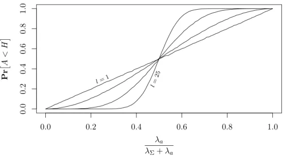
Unfortunately, it is not easy to state this probability in closed form. On the other hand, it is trivial to estimate it from a simulation. Figure 1 shows the outcome of such a simulation, using 50000 observations per parameter pair. It is worth to note, thatPrA < Hdoes not depend on the absolute values of λa and λΣ, but only on the

attackers share of solving power.

We see that for l= 1, the adversaries success probability equals its share in solving power. By increasingl, the success probability of an adversary with less than half of the solving power can be decreased and pushed towards zero. For λΣ =λa, the choice of l does not affect the success probability and for adversaries with more than half of the power, increasingl even reduces the protocol’s security.

(21)

0.0 0.2 0.4 0.6 0.8 1.0 0.0 0.2 0.4 0.6 0.8 1.0 λa λΣ+λa Pr A < H l=1 l= 25

Figure 1: Adversary’s success probability dependent on its share of solving power when using no delays (l∈ {1,2,6,25})

Delays only Now, we assume that the adversary delays messages, but is not able to produce own votes, i. e.∆>0 and λa= 0.

We analyze the following adversarial strategy. When receiving the first vote, the adversary relays it immediately to some nodes, such that the network is partitioned into two equally powerful sets. The trailing part of the network, i. e. the part that did not receive the first vote yet, might produce another vote within the maximum delay∆. If so, the partition can be maintained for more than∆ time, by letting the trailing part synchronize on the second vote, before relaying the first vote. This strategy is repeated until the protocol terminates. In the end, there must be two preferred values, each with l

votes. Since the adversary cannot produce own votes, all votes have to be generated by honest nodes.

The strategy temporally succeeds for one vote, when the trailing part of the network catches up within ∆ time. The trailing nodes produce votes at rate0.5·λΣ. Let random

variableX∼Exp(0.5·λΣ). Then, the probability of the trailing part catching up once

isPrX <∆. This has to succeed l times, each time being independent of the others. Thereby, the adversaries success probability using this strategy is Pr

X <∆l.

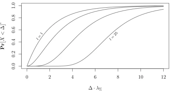
We observe, that PrX < ∆ = PrY < 0.5, where Y ∼Exp(∆·λΣ). Growing delays can be compensated by decreasing network solving power and vice versa. Figure 2 shows how the solving power measured in expected number of puzzles per network delay (∆·λΣ) affects the success probability Pr

(22)

0 2 4 6 8 10 12 0.0 0.2 0.4 0.6 0.8 1.0 ∆·λΣ Pr X < ∆ l l= 1 l= 25

Figure 2: Adversary’s success probability dependent on ∆·λΣ when using only delays

(l∈ {1,2,6,25})

We see that for low l,∆·λΣ should be near zero. This can be achieved by moderating

the puzzle such that λ∆−1. By increasingl, higher delays can be compensated. For highl, evenλ≈∆−1 is tolerable.

Combined strategy A realistic adversary would consider both techniques. It could default to the better of the two above strategies or use an even better one. Thus the two previous success probabilities constitute lower bounds.

A combined strategy might be to slow down the honest players using the second strategy, while trying to outrun their voting using the first strategy. This is the basic idea behind the so-called Selfish Mining strategy by Eyal and Sirer [14]. They proposed the strategy against a more elaborate protocol (see section 5), but the key aspects are comparable. Detailed analysis of Selfish Mining is given in [29] and [19].

(23)

5 Proceeding Consensus

In this section, we extend the consensus mechanism for single election to support an ongoing process. The previously unordered set of votes becomes an ordered list of records. Instead of electing a single value, each record contains a different value and execution is not stopped afterl records. The new protocol allows the nodes of a distributed network to find consensus on a proceeding list of values.

The previous voting mechanism is projected by counting extensions of the list as votes for the list. Voting and extending the list of values happens in parallel. Each extension needs a distinct proof-of-work, i. e. puzzle solution. This is achieved by using the complete lists as payloads for the puzzles.

Protocol 2. As before, the consensus mechanism is based on a fixed proof-of-work puzzle

(D,C, P)with verification algorithm_Verif. The procedure_Solveis a competitive solving algorithm for this puzzle.

Nodes maintain a list of values locally. Each value is in N. We refer to the list of

values as history h. Appending a value to the history requires a proof-of-work. The proofs are solutions to distinct puzzle instances and stored in a separate listp. The puzzle payloads are chosen such that a change to an historic value invalidates the successors. Together with the following validity property, the two listsh andp constitute a verifiable data structure.

valid(h, p) ⇔ |h|=|p|

∩ ∀i∈[1,|h|] :p[i]∈P(h[1, . . . , i])

Nodes follow the listing of algorithm 4. They are initialized with two empty lists and the preferred value0, using the procedure_init.

Nodes are permanently busy with solving puzzles instances. Each solved puzzle allows them to record one value in a list. Solving happens asynchronously to the rest of the algorithm. The process is started and reset using the procedure _extend. Whenever a node succeeds in extending the list, it broadcasts its extended history together with the proofs to the other nodes using the abstract procedure_send.

On the receiving side, nodes adapt the longest valid history they are aware of. Messages are pairs of lists(h, p). Receiving nodes asynchronously call procedure_receive on each received message. They verify that the received pair is valid by checking each puzzle solution, using the function_valid. If the received history is both valid and longer than their local history, they adopt the remote lists and restart their solver.

Nodes do not only interact with each other, but also with their environment. There is only one form of interaction, which allows the environment to set the preferred value and read the nodes’ local histories. The interaction is described in the procedure_request. The procedure takes a value as argument, sets it as new preferred value, restarts the solver and responds using the abstract procedure _out.

(24)

Algorithm 4Consensus on a growing history of values

1: procedure_init

2: c←0 . preferred next value, candidate

3: h←[ ] .history

4: p←[ ] .proofs

5: _extend ()

6: procedure_extend

7: terminate other instances of _extend

8: s←_Solve (h::c) . call a competitive solving algorithm

9: h←h::c 10: p←p::s 11: _send (h, p) 12: _extend () 13: procedure_request (x) 14: c←x 15: out (h::c) 16: _extend () 17: procedure_receive(h0, p0)

18: if _valid (h0, p0) and|h0|>|h|then

19: h←h0

20: extend ()

21: function_valid (h, p)

22: if |h| 6=|p|then return⊥

23: fori∈[1,|h|]do

24: if _Verif (h[1, . . . , i], p[i]) =⊥then return ⊥

(25)

5.1 Model

For the proceeding consensus, we do not only adapt the previous protocol, but also the model for the analysis. We make it bit more formal in order to reflect the strictly formal uniform composability framework [5], that is used by other blockchain protocol analyses [16, 28].

As before, we enumerate the honest participating nodes from 1ton. We will use the indicesiandj when talking about single nodes. Each honest node has a solving powerλi. Together the rates sum up toλΣ=Pλi.

Honest nodes follow protocol 2. They execute the protocols algorithm and do not modify their local states in any other way. We assume that all nodes start the execution at the same time t= 0 and are initialized using the procedure _init.

Again we assume that all computational steps except puzzle solving take zero time. The solving algorithm _Solve takes time according to the definition of the proof-of-work puzzle. We ignore problems caused by the concurrent calls to the procedures. The procedure_extend is always terminated during the call to _Solve.

Compared to the old model, communication is handled differently. Instead of giving the adversary the possibility to delay messages, we consider a worst case scenario. We allow arbitrary attackers with certain restrictions.

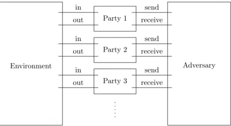
The adversary controls the network. It is responsible for message delivery. For that purpose, the procedure _send, that is used by honest nodes to broadcast messages, hands the messages over to the adversary. Only the adversary is able to hand over messages to nodes. The model assumes that it does this by invoking the_receiveprocedure on the receiving node with the message as argument.

The interaction between clients and nodes is simulated by the environment. The environment is able to make requests to each node and read their responses. The model assumes that the procedure_requestis invoked with the requested value as argument and the procedure_out hands a node’s answer over to the environment.

Figure 3 shows the described information flow in the new communication model.

Obviously, the communication model only makes sense with further assumptions. Especially the adversary has to be restricted or otherwise could simply drop all messages and prevent consensus reliably.

Thus, we assume that the adversary delivers an unaltered copy of each honestly sent message to all other nodes within maximum∆ time. Since this is the only restriction, the adversary can introduce individual delays, reorder and duplicate messages and send own messages to some nodes only. Obviously, the adversary can read all message contents and adapt its behaviour based on this knowledge.

(26)

Environment Adversary out in receive send Party 1 out in receive send Party 2 out in receive send Party 3

Figure 3: Communication model for a distributed system where the adversary is able to control the network

Executions of the protocol within the model are analyzed by observing the nodes’ outputs over time. We assume that the execution is started at timet= 0. The random process{outi,t}_t∈R+0

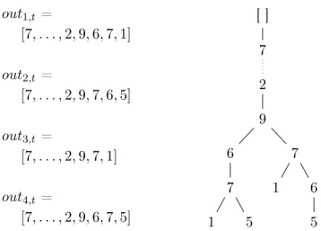
refers to the sequence of values that nodeiwould generate as output at timet.

The global view on all local outputs at time tcan be interpreted as a tree. For that purpose, consider a tree where the root node corresponds to the empty sequence and each path starting from the root corresponds to a non-empty sequence of values. From a set of sequences, the tree can be obtained by collapsing common prefixes into one path. We denote this tree view at timetastreet. The interpretation is visualized in figure 4.

The random process{treet}_t∈_R+

0 refers to this tree over time. Certain properties of

the protocol can be stated as properties of this process. For example, the inconsistency between two local views can be measured by observing the distance between the two corresponding leaves in the tree. If the local views are the same, the leaves are equal and there distance is zero. If the views are equally long and differ in the latest 3 values, the distance would between the nodes would be 6.

5.2 Desiderata

In section 4, we analysed the single election consensus protocol with respect to consistency. We rephrase consistency to fit the new protocol and model. Additionally, we add two more properties – growth and quality – that allow to derive persistence and liveness of an Bitcoin-like application build on top.

Together, the three properties ensure that the distributed system reaches consensus and stays operational. Consistency ensures, that disputes on the history are settled over time. Quality implies, that not only adversarial values are included in the history. Growth implies progress. At least some honest values will be included and the system is operational.

(27)

out1,t = [7, . . . ,2,9,6,7,1] out2,t = [7, . . . ,2,9,7,6,5] out3,t = [7, . . . ,2,9,7,1] out4,t = [7, . . . ,2,9,6,7,5] [ ] 7 2 9 6 7 1 5 7 1 6 5

Figure 4: Correspondence between global tree viewtreet and local viewsouti,t

The random nature of the execution, does not allow for absolute security guarantees. We will express all three properties by saying a certain condition is true with high probability. By increasing a security parameter, the probability of violation will be decreased.

For that purpose, we use the concept of negligible functions. A function :R→R+0

is negligible if for any polynomial p, there exists xp such that (x)·p(x) ≤ 1 for all x≥xp. This means, that a negligible function goes faster to zero than the inverse of any polynomial.

We have previously seen (section 4.2), that the security of a proof-of-work protocol can be improved, by increasing the amount of necessary votes. We transfer this concept to the new model by observing growing subsequences of the history. Growing the observed window corresponds to increasing the amount of votes. With a bigger window comes a higher probability of consistency, quality and growth.

For l∈_N and two sequencess0 ands1, lets0=ls1 denote that s0 ands1 are equal in

all but the lastl entries. Formally,

s0=ls1 ⇐⇒ ∀ k≤min(|s0|,|s1|)−l:s0[k] =s1[k].

Property 1 (Consistency). A protocol ensures consistency if there exists a negligible function1, such that for any two pointst0 andt1 in time, and for any two honest nodesi

and j,

Pr

outi,t0 =loutj,t1

≥1−1(l) .

The consistency property is similar to the consistency goal for the single election consensus in section 4. It says that all honest nodes end up in the same state after some time. Instead of an unordered set of votes for a value, we now count the number l of confirmations, i. e. the number of records that happened after a potential segmentation. With more confirmations, the probability of inconsistency goes down quickly.

(28)

We note, that the above statement allows j = i and thus implies self-consistency. Except for the last lentries, the local states do not over time.

Property 2(Growth). A protocol ensuresg-growth if there exists a negligible function2,

such that for any two pointst0 andt1 in time witht0+ ∆≤t1,

Prmin

i,j (|outi,t1| − |outj,t0|)≥g·(t1−t0)

≥1−2(t1−t0) .

The growth property gives a lower bound on the growth rate of the history. It ensures that records are added over time and prevents the adversary from stopping the proceeding consensus.

The growth property is stated relative to the sizes of the observed time window. By increasing the time window, the probability that less than g·sentries were added during this time, goes quickly towards zero. In terms of the global tree view, this means that the number of levels of the tree is growing over time at a minimum rateg.

At last, we consider how may entries are added by honest participants. We say, that an entry is honest, if it was requested for inclusion by the environment before being recorded. The amount of such honest entries should be high.

Let hl_m(outi,t)denote the number of honest records in the segment of lengthlofouti,t starting at the m-th record.

Property 3(Quality). A protocol ensuresµ-quality if there exists a negligible function3,

such that for any time t0 and honest node i,

Prhl_m(outi,t0)≥µ·l

≥1−3(l) .

The quality property ensures that the adversary cannot continuously write its own values into the persistent history. At least a certain fraction of the entries can be attributed to the honest part of the network.

The property is stated with respect to a function negligible in the length of the observed segment of the list. When increasing this lengthl, the probability that a local view contains less thanµ·lhonest entries goes towards zero quickly.

5.3 Analysis

Compared to the protocol for a single election, protocol 2 introduces new features, but does not address the previously analyzed security problems. Additionally, the new model allows for more capable adversaries. In section 4.2, we gave lower bounds on the adversaries success probability, when attempting to interrupt consensus. Intuitively, these lower bounds also apply to the new protocol. It is likely, that new problems have been introduced.

Indeed, the new protocol makes it easier to exploit selfish mining. The idea of such an attack is to use network delays and holding back of solutions to trick honest miners into extending stale sets of votes or, in this case, stale histories. Previously, chances where

(29)

high, that this succeeds only on the first few votes. The honest nodes synchronized their preferred value after the first missed catch-up by the adversary. There was no way of introducing new inconsistency into the states of honest nodes.

Now, the situation is different. With the new protocol, the adversary can fork the history at any point and thereby reintroduce inconsistency. Honest miners thus continuously waste their solving power on irrelevant puzzles. Other analyses [14, 29] show, that a selfish miner can effectively double its solving power by using a dishonest strategy. A share of one third of the global solving power enables the adversary to contribute on half of the records.

Nevertheless, it should be possible to show that protocol 2 fulfills the above properties with respect to an adversary that is limited to less than half of the overall solving power. Conjecture 1. Let α < 1₂ and the puzzle be moderated such that ∆ 1

λΣ. Then,

protocol 2 ensures consistency,λΣ-growth and(1−₁₋1_α)-quality.

This statement is proven for a similar protocol in the related models of Garay et al. [16] and Pass et al. [28]. We think, that their proofs are transferable to our model.

5.4 Related Work

In this section we introduced a less formal version of the universal composability (UC) framework. In the original work by Canetti [5] nodes are represented by interactive Turing machines (ITM). Each machine has four communication tapes. The_input and_output tapes are used for communication between environment and nodes. The environment can write requests to _input and read answers from _output. The two tapes_receiveand sendare communication between the nodes. Both the environment and the adversary are modelled as arbitrary ITMs with some restrictions.

An overlay broadcast network with guaranteed message delivery after ∆ time can be modelled by connecting the adversarial ITM A to the nodes communication tapes send and receive and let it handle delivery alone. Malicious behaviour is modelled by allowing all such ITMs forA that deliver an unaltered copy of scheduled messages within ∆time to all other nodes.

The security properties stated in section 5.2 follow the work on the Bitcoin backbone protocol by Garay et al. [16] and Pass et al. [28], who state and proof their statements in the UC framework. The former introduce an abstract blockchain protocol. They fomulate the common prefix and quality properties and proof them for their protocol using the random oracle model. They work in the synchronous setting, where messages are delivered at the end of each round. They also allow honest nodes turning rogue during execution. Pass et al. [28] explicitly add the growth property and provide proofs for all three properties in a model using a custom Ftree oracle. This oracle simulates success on extending the data structure and allows to proof the security properties in the partially asynchronous setting, where the network delay ∆may be greater than one round, but must be known a-priori. They further show that proofing properties for the random oracle based Bitcoin backbone protocol can be reduced to statements in the Ftree model. They thereby confirm and generalize the results of Garay et al. [16].

(30)

6 Practical Aspects

In section 5, we presented a basic protocol for consensus on a growing list of values. This section explores, how actual applications can be built on top of this mechanism. We start by explaining the concept of state machine replication. It allows to implement a wide range of services using the proceeding proof-of-work protocol. Afterwards, we discuss two protocol optimizations that improve performance and scalability of such distributed state machines. Although not highlighted as such, both optimizations were part of the original proposal for Bitcoin [25] and are used in all other practical implementations.

6.1 State Machine Replication

An append-only list of values can be leveraged to represent the execution of an arbitrary application using state machine replication. For that purpose, the application has to be defined as a state machine. The consensus protocol is then used for the distributed execution of the machine. Instead of recording integer values into the history, the protocol reasons on state transitions. With each recorded event, the state is updated. When nodes eventually agree on the same history up to a certain record, they thereby agree on the state of the machine at that point in time.

The concept of state machine replication is much older than consensus based on proof-of-work. Lamport [20] first proposed it in 1978 in the context of Byzantine fault tolerant protocols. He proposed, that Byzantine faults should be used to analyze the reliable exchange and ordering of messages. A distributed state machine could then be implemented on top. Later, Schneider [30] surveyed on the concept.

One example for a application based on state machine replication and proof-of-work consensus is the cryptocurrency Bitcoin [25]. Its global state describes a set of unused, previous transaction outputs. Each such unspent transaction output (UTXO) defines a value and an unlock condition. State updates are defined as small transaction scripts. Each script can contain an input that satisfies the unlock conditions of one or more UTXO. Unlocked values can be reassigned to fresh unlock conditions and thereby create fresh UTXOs.

The use of asymmetric cryptographic primitives in the transaction script enables to lock values such that a private key is necessary in order to satisfy the unlock condition. This allows to model accounts with balances, where solely the account holder is able to move parts of their balances to other accounts.

The smart contract platform Ethereum [32] takes the transaction logic one step further. State updates may persist program code in the history. Subsequent transactions can invoke functions specified within the persisted code. The program code is then executed with arguments from the calling transaction. This essentially allows to define new state machines deploy them for execution on top of Ethereum. Such applications are called smart contracts and can contain arbitrary business logic.

Unfortunately, the state machine replication approach allows application developers to quickly exceed the scalability bounds of the underlying consensus protocol. The theoretical protocol 2 requires to solve one proof-of-work puzzle per recorded value and broadcasts

(31)

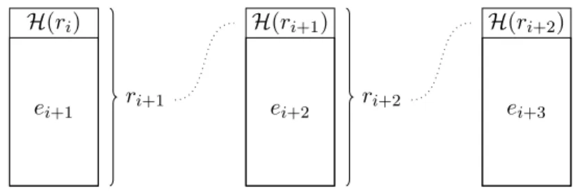
H(ri) ei+1 ri+1 H(ri+1) ei+2 ri+2 H(ri+2) ei+3

Figure 5: Elementsei+1 to ei+3 stored in a hash-linked list

the complete history of values with each found puzzle solution. In this new setting, where values are updates to distributed state machine and the list of state updates may grow forever, it can be considered a deal-breaker.

Fortunately, there are two optimizations that allow to overcome these problems. Practical implementations allow to bundle multiple events in blocks and avoid retransmis-sion of history using hash-linked lists. In sections 6.2 and 6.3, we will discuss the two optimizations separately.

6.2 Hash-Linked List

Following the protocol for proceeding consensus as presented in section 5 nodes broadcast the complete history of records with each found puzzle solution. The message size grows linear in time.

We have seen that the security of the mechanism depends on the maximal network delay∆. Naturally, the growing message size negatively affects the latency. As is, the protocol is unsuitable for long-term operation.

The message overhead can be significantly reduced by storing the records in a hash-linked list. Instead of retransmitting the whole history of events together with their proofs, only a short identifier thereof is sent over the network. These identifiers are constructed from a random oracle or a cryptographic hash function in practice.

A hash-linked list is data structure that is well suited for append-only data. It is similar to a reverse linked list. Instead of storing a pointer to the previous element, a hash of the predecessor is included in each appended elements. The concept is illustrated in figure 5.

Definition 8 (Hash-linked list). LetH:Bl×D→Bl be a random oracle. A sequence

s∈(Bl×D)n is called ahash-linked list of length n∈_N if

∀ i∈[2, n] :H(si−1) =f(si) ,

wheref maps a tuple to its first element. Dis the set of storable elements.

A central property of hash linked lists is that a change to one element of the list cuts off all successors. If an element is changed, its hash changes too. All incoming links from successors are broken. Assume element eis changed to e0. The successors was linked

(32)

toeby including the hash H(e). After the change, edoes not exist any more andH(e)

is an invalid reference. In order keep the structure of the list, s has to be updated to includeH(e0). Inductively, the same is true for all successors.

The appending of new elements can be communicated without transmitting the whole list. Fresh elements are bound to exactly one list of predecessors. Thus it is enough to send only the new element over the network. Receiving parties can infer from the included hash-link, which list has to be extended. For our consensus protocol this implies, that the transmission of new events and hash links is enough to remotely synchronize local states.

Algorithm 5 shows a modification of protocol 2 using a hash linked list. Instead of keeping proofs and events separately, everything is kept in a map using the hash of its element as keys. The modification reduces the message space from(E× C)∗ toE×Bl× C

and thereby eliminates a major scalability problem of the consensus mechanism. Instead of being proportional to the length of the history (and thereby time) the length of messages is now constant.

The presented modification of the consensus protocol relies on collision and second preimage resistance ofH. Collision resistance ensures that no two records have the same hash and each hash reference links to a unique predecessor. Missing collision resistance would lead to ambiguities in the order of the list. Second preimage resistance ensures that changes to a record break the connection to all successors of this record. Without second preimage resistance it might be possible to change a record while keeping its hash the same. This would allow for modification of the history.

6.3 Bundling Events in Blocks

Protocol 2 records values one by one. When using state machine replication to implement a distributed service, the throughput is limited to one state update per solved puzzle instance. In order to allow the network to synchronize between recorded events, the average time between found solutions must be long compared to the maximum network delay∆. Thus, the overall throughput is very low.

One way around this limitation is to bundle multiple events in blocks and treat them as a single record. For that purpose, the environment facing part of the protocol can be modified to accumulate incoming requests. Nodes order incoming events locally, execute them, check for conflicts and put them into a temporary list. The puzzle is constantly updated to match the list. As soon as a puzzle solution is found, the block of events is broadcasted to the other nodes and the node starts to build a new block from scratch.

Algorithm 6 shows the necessary changes. In practice this would be combined with the changes introduced in section 6.2, but we skip this in order to avoid convolution.

In practice, the proposed protocol extension is accompanied by a second synchronisa-tion mechanism on the level of transacsynchronisa-tions or events. After receiving a transacsynchronisa-tion from the environment, honest nodes broadcast it to the rest of the network. This allows all nodes to include a transaction equally. Inclusion happens on the next few blocks in the network instead of the next block of the nodes that received the transaction from the environment.