Accurate Segmentation of CT Male Pelvic Organs via
Regression-based Deformable Models and Multi-task Random
Forests
Yaozong Gao,
Department of Computer Science, the Department of Radiology and Biomedical Research Imaging Center, University of North Carolina, Chapel Hill, NC 27599 USA ([email protected])
Yeqin Shao,
Nantong University, Jiangsu 226019, China and also with the Department of Radiology and Biomedical Research Imaging Center, University of North Carolina, Chapel Hill, NC 27599 USA ([email protected])
Jun Lian,
Department of Radiation Oncology, University of North Carolina, Chapel Hill, NC, 27599 USA
Andrew Z. Wang,
Department of Radiation Oncology, University of North Carolina, Chapel Hill, NC, 27599 USA
Ronald C. Chen, and
Department of Radiation Oncology, University of North Carolina, Chapel Hill, NC, 27599 USA
Dinggang Shen [Senior Member, IEEE]
Department of Radiology and Biomedical Research Imaging Center, University of North Carolina, Chapel Hill, NC 27599 USA and also with Department of Brain and Cognitive Engineering, Korea University, Seoul 02841, Republic of Korea ([email protected])
Abstract
Segmenting male pelvic organs from CT images is a prerequisite for prostate cancer radiotherapy. The efficacy of radiation treatment highly depends on segmentation accuracy. However, accurate segmentation of male pelvic organs is challenging due to low tissue contrast of CT images, as well as large variations of shape and appearance of the pelvic organs. Among existing segmentation methods, deformable models are the most popular, as shape prior can be easily incorporated to regularize the segmentation. Nonetheless, the sensitivity to initialization often limits their performance, especially for segmenting organs with large shape variations. In this paper, we propose a novel approach to guide deformable models, thus making them robust against arbitrary initializations. Specifically, we learn a displacement regressor, which predicts 3D displacement from any image voxel to the target organ boundary based on the local patch appearance. This regressor provides a nonlocal external force for each vertex of deformable model, thus overcoming the initialization problem suffered by the traditional deformable models. To learn a reliable displacement regressor, two strategies are particularly proposed. 1) A multi-task random forest is
HHS Public Access
Author manuscript
IEEE Trans Med Imaging
. Author manuscript; available in PMC 2017 June 01.Published in final edited form as:
IEEE Trans Med Imaging. 2016 June ; 35(6): 1532–1543. doi:10.1109/TMI.2016.2519264.
A
uthor Man
uscr
ipt
A
uthor Man
uscr
ipt
A
uthor Man
uscr
ipt
A
uthor Man
uscr
proposed to learn the displacement regressor jointly with the organ classifier; 2) an auto-context model is used to iteratively enforce structural information during voxel-wise prediction. Extensive experiments on 313 planning CT scans of 313 patients show that our method achieves better results than alternative classification or regression based methods, and also several other existing methods in CT pelvic organ segmentation.
I. Introduction
Prostate cancer is a common type of cancer in American men. It is also the second leading cause of cancer death, behind only lung cancer, in American men [1]–[3]. External beam radiotherapy is one of the most effective treatments for prostate cancer. In the planning stage, delineation of organs at risk is a crucial task for radiation oncologists. Radiation fields are optimized with the goal of delivering the prescribed dose to the prostate volume, while sparing nearby healthy organs, such as bladder, rectum, and femoral heads. Manual delineation is normally adopted in most clinical practices, but is a time-consuming and labor-intensive process, typically taking 27–33 minutes for an experienced radiation oncologist to delineate target (prostate) and four major organs of risk, including bladder, rectum and two femoral heads. Moreover, manual delineation often suffers large inter-operator variability [4], [5]. Accordingly, it is clinically desirable to develop a robust, accurate and automatic algorithm for the segmentation of major male pelvic organs from CT images.
It is generally difficult to automatically segment male pelvic organs from CT images due to three challenges, as illustrated in Fig. 1. 1) Male pelvic organs exhibit low contrast in CT images. For example, the organ boundaries are often indistinct, especially when two nearby organs touch together. 2) The shapes of bladder and rectum are highly variable. They can change significantly across patients due to different amounts of urine in the bladder, and bowel gas in the rectum. 3) The rectum appearance is highly variable due to the uncertainty of bowel gas and filling.
Many methods have been proposed to address the aforementioned challenges, such as deformable models [5]–[11], deformable registration [4], [12] and multi-atlas-based labeling [13]. A few methods [8], [12], [13] achieved high segmentation accuracies by exploiting patient-specific information from the previous CT scans of the same patient. However, these methods cannot be directly applied to segment the planning CT scans due to the
unavailability of such patient-specific data in the beginning. In addition, most existing works [4], [6], [7], [9] segmented only one or two major pelvic organs. It is unclear whether these methods can be extended to segment other pelvic organs with good performance. Also, there are few works [5], [10] that simultaneously segment three major pelvic organs, including prostate, bladder and rectum. Although [10] obtained a good segmentation accuracy on the prostate, their performance on the bladder and rectum is still limited mainly because of the difficulty in robust model initialization for organs with highly variable shapes. The same situation applies to [5]. Since prostate cancer radiotherapy focuses on not only maximizing the dose to the prostate, but also minimizing the dose to the nearby healthy organs, it is critical to accurately segment the bladder, rectum and femoral heads, in addition to the
A
uthor Man
uscr
ipt
A
uthor Man
uscr
ipt
A
uthor Man
uscr
ipt
A
uthor Man
uscr
prostate. Radiation therapy based on inaccurate segmentation of these organs would result in severe side effects, such as persistent bleeding from the bladder and rectum [14], [15], and femoral head necrosis [16].
To this end, we propose novel regression-based deformable models to segment male pelvic organs from CT images. Compared to the conventional deformable models, the contributions of our work are three-fold:
• We propose to learn a displacement regressor for guiding deformable segmentation. Different from existing deformable models [5], [7], [8], [10], which deform each vertex by locally searching the maximum boundary response, we use the underlying image patch of each vertex to estimate a 3D displacement, pointing to the nearest voxel on the target organ boundary, for guiding shape deformation. Compared with local search, the estimated displacement provides a non-local external force, thus making our deformable models robust to initialization.
• We propose a multi-task random forest, which jointly learns the displacement regressor and organ classifier. Compared to random forest regression or classification, the proposed multi-task random forest is better in estimating displacement fields and organ classification maps.
• We re-discover the auto-context model [17] as a structural refinement method. In particular, we use it to iteratively refine the estimated displacement fields by injecting the structural prior learned from training images.
The extensive experiments on 313 CT scans of prostate cancer patients demonstrate that our method can accurately segment male pelvic organs from planning CT images, and
outperforms the published state-of-the-art methods, especially for the bladder and rectum, whose shapes are highly variable. To the best of our knowledge, this is the most accurate automatic method for segmenting male pelvic organs from planning CT images yet reported. Also, this is the largest dataset ever used in the literature for evaluating such automatic segmentation methods.
The rest of the paper is organized as follows. Section II gives an overview of related methods on both CT pelvic organ segmentation and learning-based deformable
segmentation. Section III presents different components of our method, including multi-task random forest, iterative structural refinement and regression-based deformable model. The experimental results are provided in Section IV. Finally, Section V presents the conclusion.
II. Related Works
As mentioned, we propose regression-based deformable models for segmenting male pelvic organs in CT images. The following literature review will cover both CT male pelvic organ segmentation and learning-based deformable models, respectively.
A
uthor Man
uscr
ipt
A
uthor Man
uscr
ipt
A
uthor Man
uscr
ipt
A
uthor Man
uscr
A. CT Male Pelvic Organ Segmentation
The segmentation of male pelvic organs from CT images has been investigated for a long time. Most of existing methods can be categorized into two groups, i.e., planning CT segmentation and treatment CT segmentation.
1) Planning CT Segmentation—Costa et al. [7] proposed a coupled deformable model for jointly segmenting the prostate and bladder by considering the non-overlapping constraint. Chen et al. [9] incorporated anatomical constraints from pelvic bones to segment the prostate and rectum. Lu et al. [10] combined a learning-based boundary detector with the Jensen-Shannon divergence for deformable segmentation of the prostate, bladder and rectum. Lay et al. [5] proposed to integrate local and global image context for fast segmentation of five pelvic organs from CT images.
However, due to the aforementioned challenges, the performance of most existing works is limited. In addition, many works [6], [7], [9] were specially designed for segmenting one or two pelvic organs. It is difficult to extend these methods for segmenting other pelvic organs. To avoid handcrafting methods, recent works [5], [10] showed the potential of machine learning techniques to address this segmentation problem. While these methods showed some effectiveness in segmenting organs with small shape and appearance variations, such as the prostate, their performances are still limited for organs with highly variable shapes, such as the bladder and rectum, because of the difficulty in initialization of deformable model.
2) Treatment CT Segmentation—Different from planning CT segmentation, the treatment CT segmentation can exploit the previous CT scans of the same patient to improve segmentation performance. Foskey et al. [4] segmented the prostate by deformable
registration of the segmented planning CT scan of the same patient onto the treatment image. Feng et al. [8] adopted a deformable model, which leverages both population and patient-specific statistics for segmenting the prostate. Gao et al. [18] proposed to incrementally learn landmark detectors from patient-specific CT scans for rapid prostate localization.
Although these methods obtained promising results on treatment CTs, they often require contours on one or more previous CT scans of the same patient to learn patient-specific appearance/shape models. This requirement renders them inapplicable to segmenting pelvic organs in the planning CTs, where no such patient-specific data are available in the
beginning.
B. Learning-based Deformable Models
Deformable models are popular methods for medical image segmentation. In this paper, we focus on 3D parametric deformable models represented by triangle meshes. In the
conventional deformable models, each vertex of a shape model deforms locally along the inward and outward normal directions to a position with the maximal boundary response. Instead of using intensity or gradient profiles to characterize boundaries [19], many
researches [5], [10], [20] have shown that learning a classifier to distinguish boundary voxels
A
uthor Man
uscr
ipt
A
uthor Man
uscr
ipt
A
uthor Man
uscr
ipt
A
uthor Man
uscr
from non-boundary voxels is more effective, especially for organs with indistinct boundaries. However, since each vertex still deforms locally, deformable models are sensitive to initialization, no matter whether intensity profiles or classifiers are used for boundary detection. Actually, the performance of deformable models is highly dependent on whether good initializations can be obtained. Accordingly, many researches have been conducted to address the initialization problem. Roughly, they can be categorized into two types, i.e., landmark-based initialization and box-based initialization, as briefly described below.
1) Landmark-based Initialization—Zhang et al. [21] adopted a boosting framework for landmark detection. The detected landmarks are used in the sparse shape composition to infer a rough shape for deformable model initialization. Gao et al. [22] proposed a two-layer regression forest to enforce spatial consistency between detected landmarks, which are then used for fast prostate initialization.
Despite the effectiveness, landmark-based initialization is often applicable only to organs with small shape variations, such as the bones and prostate. For organs with large shape variations and irregular shapes, such as the bladder and rectum, it is often difficult to define landmarks consistently across subjects, thus making landmark-based initialization less effective.
2) Box-based Initialization—There are two typical methods for box-based initialization. Criminisi et al. [23] proposed to use regression forest for detecting axis-aligned bounding boxes of organs in CT images. The detected bounding box can be used to initialize the position and scale of deformable model. Zheng et al. [24] proposed “marginal space learning” for detecting oriented bounding boxes of organs, which provides not only position and scale, but also orientation of the target organ.
Compared with landmark-based initialization, box-based initialization is more universal for deformable model initialization, as it is easy to define the 3D bounding box of an organ and does not suffer from the consistency issue like landmark-based initialization does. However, for organs with irregular shapes, such as tubular shapes of the rectum, a bounding box may be too rough to be considered as a good initialization. Moreover, as validated in IV-F, we found that bounding box detection does not work well for the bladder, whose shape is highly variable across subjects.
To summarize, the performance of most deformable models heavily depends on
initialization. While many learning-based methods have been proposed to address this issue, so far it is still a challenging problem to robustly initialize deformable models, especially for organs with highly variable and irregular shapes. Therefore, we think that the problem will not be essentially solved by merely improving initialization. To resolve this problem, it is necessary to change the local deformation mechanism of deformable models.
A
uthor Man
uscr
ipt
A
uthor Man
uscr
ipt
A
uthor Man
uscr
ipt
A
uthor Man
uscr
III. Method
A. Overview
As shown in Fig. 2, our method consists of two major steps, i.e., 1) displacement field estimation and 2) regression-based hierarchical deformation. The following sections are organized as follows: Section III-B describes displacement field estimation by a multi-task random forest, which learns the displacement regressor jointly with the organ classifier. Section III-C describes how structural priors can be injected into voxel-wise prediction by the auto-context model. Finally, Section III-D presents the regression-based hierarchical deformation for segmentation.
B. Multi-task Random Forest
Conventional random forest [25] focuses only on one task, such as regression or
classification. Recent researches on multi-task learning [26] suggest that learning related tasks in parallel using a shared representation could improve the generalization of learned model. Moreover, what is learned for each task can help other tasks to be learned better. Inspired by this idea, we propose a multi-task random forest for predicting the 3D displacement field.
In this paper, we consider two tasks, displacement regression and organ classification. The inputs of the two tasks are the same, which is a local patch centered at the query voxel. The difference between the two tasks is the prediction target. Displacement regression aims to predict a 3D displacement pointing from the query voxel to the nearest voxel on the boundary of target organ, while organ classification aims to predict the label/likelihood of the query voxel belonging to a specific organ (e.g., bladder). An illustration is given in Fig. 3. It is not difficult to see that these two tasks are highly related, since displacement field and classification map are just two representations of organ boundary.
To adapt random forest for multi-task learning, we modify the objective function of random forest as follows:
(1)
where f and t are the feature and threshold of one node to be optimized, respectively. wi is
the weight for each task. Gi is the gain of each task by using { f, t} to split training data
arriving at this node into left and right children nodes. Since we consider only two tasks, i.e., displacement regression and organ classification, the objective function can be further specialized as follows:
A
uthor Man
uscr
ipt
A
uthor Man
uscr
ipt
A
uthor Man
uscr
ipt
A
uthor Man
uscr
(2)
where υ, e and N are the average variance over displacement vector, the entropy of class label and the number of training samples at the current node, respectively. Symbols with superscript j ∈ {L, R} indicates the same measurements computed after splitting into left or right child node. Gregress is the gain of displacement regression, which is measured by
variance reduction. Gclass is the gain of organ classification, which is measured by entropy
reduction. Since the magnitudes of variance and entropy reductions are not of the same scale, we normalize both magnitudes by dividing the average variance and entropy at the root node (Zυ and Ze), respectively.
With this modification (Eq. 2), random forest is optimized for both displacement regression and organ classification, which means that we can use one random forest to jointly predict the 3D displacement and the organ likelihood of a query voxel. Compared to separate displacement regression and organ classification by conventional random forest, multi-task random forest could utilize the commonality between these two tasks, thus often leading to better performance. Experimental results (Section IV-D) also show that displacement regression and organ classification are mutually beneficial if jointly learned in the multi-task random forest.
Features—The input of the multi-task random forest is a local patch centered at the query voxel. The output is the 3D displacement from the query voxel to the nearest voxel on the boundary of target organ, and the likelihood of the query voxel belonging to the target organ. Since CT images are very noisy, it is unwise to directly use local intensity patch as features. A common practice is to extract several low-level appearance features from the local patch and use them as input to random forest. Among various features, we choose Haar-like features because they are robust to noises and can be efficiently computed using the integral image [27]. In this paper, we consider two types of Haar-like features: 1) one-block Haar-like features compute the average intensity at one location within the local patch; 2) two-block Haar-like features compute the average intensity difference between two locations within the local patch. Their mathematical definitions can be formulated as follows:
(3)
where Ix denotes a local patch centered at voxel x, f (Ix|c1, s1, c2, s2) denotes one Haar-like
feature with parameters {c1, s1, c2, s2}, where c1∈ℝ3 and s
1 are the center and size of the
positive block, respectively, and c2∈ℝ3 and s2 are the center and size of the negative block,
A
uthor Man
uscr
ipt
A
uthor Man
uscr
ipt
A
uthor Man
uscr
ipt
A
uthor Man
uscr
respectively. λ ∈ {0, 1} is a switch between two types of Haar-like features. When λ = 0, Eq. 3 becomes one-block Haar-like features. When λ = 1, Eq. 3 becomes two-block Haar-like features. Fig. 4 below gives the graphical illustration of Haar-like features used in this paper.
In the training stage, we train each binary tree of random forest independently. For each tree, a bunch of Haar-like features is generated by uniformly and randomly sampling parameters of Haar-like features, i.e., {c1, s1, c2, s2}, under the constraint that positive and negative
blocks should stay inside the local patch. These random Haar-like features are used as feature representation for each training sample/voxel. As random forest has built-in feature selection mechanism, it will select the optimal feature set, which are useful for both displacement regression and organ classification.
C. Iterative Structural Refinement by the Auto-context Model
Given a new testing image, multi-task random forest can be used to voxel-wisely estimate the 3D displacement field and organ classification/likelihood map. However, since both displacement and organ likelihood of each voxel are predicted independently from those of nearby voxels, the estimated displacement field and organ likelihood map are often noisy, as shown in the first row of Fig. 5(a). To overcome this drawback, neighborhood structural information needs to be considered during voxel-wise prediction.
A Revisit of Auto-context—Auto-context [17] is a classification refinement method that builds upon the idea of stacking. It uses an iterative procedure to refine likelihood map from voxel-wise classification. For simplicity, the following paragraphs explain the auto-context model in the case of binary classification. Later we will show that it is easy to extend it for multi-task random forest.
Training—The training of auto-context typically takes several iterations, e.g., 2–3 iterations. A classifier is trained at each iteration. In the first iteration, appearance features (e.g., Haar-like features) are extracted from CT image and used together with the ground-truth label of each training voxel to train the first classifier. Once the first classifier is trained, it is applied to each training image to generate a likelihood map. In the second iteration, for each training voxel, we extract not only appearance features from CT image, but also Haar-like features from the tentatively estimated likelihood map. These features from likelihood map are called “context features”, because they capture the context information, i.e., neighborhood class information. With the introduction of new features, a second classifier is trained. As the second classifier considers not only CT appearance, but also neighborhood class information, it often leads to a better likelihood map. Given a refined likelihood map by the second classifier, the context features are updated and can be used together with the appearance features to train the third classifier. The same procedure is repeated until the maximal iteration is reached. Because each iteration involves voxel-wise classification of all training images, it takes long time for training. In practice, 2–3 iterations are often used.
Testing—Given a new testing CT image, the learned classifiers are sequentially applied. In the first iteration, the first learned classifier is voxel-wisely applied on the testing image to
A
uthor Man
uscr
ipt
A
uthor Man
uscr
ipt
A
uthor Man
uscr
ipt
A
uthor Man
uscr
generate a likelihood map by using only appearance features. In the second iteration, the second learned classifier is used to predict a new likelihood map by combining appearance features from CT image with context features from the likelihood map of the previous iteration (Fig. 5). This procedure is repeated until all learned classifiers have been applied. The likelihood map output by the last classifier is the output of the auto-context model. Fig. 6 provides the schematic diagram.
Our study shows that the context features encode neighborhood structural information, which can be used to enforce the structural priors learned from training images. To justify this statement, we conduct a synthetic experiment for shape refinement. In this experiment, given a binary training image, which represents a shape, a sequence of random forest classifiers is trained in the same manner of auto-context. Then, we sequentially apply the learned classifiers onto a testing image with a different shape. Our assumption is that, if the classifiers learn the neighborhood structural information of the training shape, the testing shape would gradually evolve to be the training shape under the iterative classification. Fig. 5(b) gives the results for two cases, where the training shapes are the prostate and the bladder, respectively. We can see that the testing shapes refined by the auto-context are almost identical to the respective training shapes, which indicates that the structural information of training images can be enforced in the testing image by the auto-context model.
To extend the auto-context model for multi-task random forest, we extract context features (i.e., Haar-like features) not only from likelihood map, but also from 3D displacement field, as illustrated in Fig. 5(a). Since context features capture the structural prior of training images, by extracting them from both likelihood map and displacement field, we can enforce the structural prior on both prediction maps during voxel-wise estimation. As shown in the bottom row of Fig. 5 (a), the likelihood map and displacement field are significantly improved by the auto-context model.
D. Regression-based Hierarchical Deformation
Given a 3D displacement field estimated by multi-task random forest with auto-context, we can use it to guide a deformable model for organ segmentation. In this paper, we propose a hierarchical deformation strategy. To start segmentation, the mean shape model, calculated as the average of all training shapes, is first initialized on the center of a testing image (Fig. 2). During deformable segmentation, initially the shape model is only allowed to translate under the guidance from estimated displacement field. Once it is well positioned, we start to estimate its orientation by allowing it to rigidly rotate. Afterwards, the deformation is further relaxed to the affine transformation for estimating the scaling and shearing parameters of the shape model. Finally, the shape model is freely deformed under the guidance from the displacement field. Alg. 1 below provides the details of our regression-based hierarchical deformation strategy. It should be noted that the jointly estimated likelihood map is not used in the segmentation stage. In this paper, the organ classification task is used only to help the task of displacement regression.
Compared to conventional deformable models, the proposed regression-based deformable models have several advantages:
• Non-local deformation: Different from conventional deformable models, deformation is no longer local in the regression-based deformable models. The non-local deformation eliminates the need to specify the search range, which is often required in the conventional deformable models [28]. On the other hand, shape models, which are even initialized far away from the target organ, can still be rapidly deformed to the correct position, under the guidance from the estimated displacement field.
• Robust to initialization: An immediate benefit of nonlocal deformation is the robustness of regression-based deformable models to arbitrary initializations. In our case, it is sufficient to initialize the mean shape model on the image center, which is almost impossible for conventional deformable models to work in most applications.
• Adaptive deformation parameters: The deformation direction and step size of each vertex is adaptively determined at each iteration for optimally driving the shape model onto the target organ. This is different from conventional deformable models, which use a fixed deformation direction (e.g., normal direction) and step size. The adaptive deformation parameters make deformable models fast to converge and also less likely to fall into local minima.
In summary, regression-based deformable models provide non-local deformations, which make them insensitive to initializations. Besides, many important designs, such as search range, deformation direction, and step size, are either eliminated or automatically determined for each vertex according to the learned displacement regressor. Therefore, regression-based deformable models have much fewer parameters to tune than the conventional deformable models.
E. Multi-resolution Segmentation
To improve the efficiency and robustness of our method, the segmentation is conducted in multi-resolution. In total four resolutions are used.
Training—In the two coarsest resolutions, one multi-task random forest is trained jointly for all five organs. Specifically, the target displacement to predict is a concatenation of 3D displacements to all five pelvic organs. The entropy in Eq. 2 is measured over a multi-class distribution, where each class is a pelvic organ. Joint estimation of all displacement fields is beneficial to consider the spatial relationship between neighboring organs. In the two finest resolutions, one multi-task random forest is trained separately for each organ. Compared to the common random forest in the coarsest resolutions, learning an individual random forest captures specific appearance characteristics of each organ, which is more effective for detail boundary refinement of the shape model.
Testing—The testing image is first down-sampled to the coarsest resolution (voxel size 8 × 8 ×8 mm3), where rough segmentations of the five organs can be rapidly obtained by our method. These segmentations serve as good initializations for the next finer resolution. The
A
uthor Man
uscr
ipt
A
uthor Man
uscr
ipt
A
uthor Man
uscr
ipt
A
uthor Man
uscr
segmentation is then sequentially performed across different resolutions, until it reaches the finest resolution (voxel size 1 × 1 ×1 mm3), where the final segmentation is achieved.
Algorithm 1
Regression-based Hierarchical Deformation
Data: I - testing CT scan, - learned multi-task random forest, and init - initialized shape model
Result: - the final segmentation
Notation: World2Voxel(I, p) outputs voxel coordinate of vertex p on image I, (I, x) returns the 3D
displacement of voxel x on the image I, and Θ (K) denotes valid transform matrix set under transform type K
Subroutine Deform(I, , , K)
for Iteration ← 1 to MaxIteration do
deform =
foreach vertex p ∈ deform do
x = World2Voxel(I, p)
p = p + (I, x)
end
if K ∈ {Translation, Rigid, Affine} then Estimate transform matrix T ∈ℝ4×4:
argminT‖T ( ) − deform‖2, s.t., T ∈Θ (K)
= T ( )
else
= SmoothSurface( deform)
= RemeshSurface( )
end end
return
Algorithm HierarchicalDeform (I, , init)
=Deform(I, , init, “Translation”)
=Deform(I, , , “Rigid”) =Deform(I, , , “Affine”) =Deform(I, , , “FreeForm”)
return
The benefits of the multi-resolution strategy are straightforward. Instead of computing the displacement field for the whole image in the fine resolution, now only a sub-region of the displacement field around the initialization (given by the previous coarser resolution) has to be computed, thus significantly improving the efficiency. Apart from the efficiency, the
A
uthor Man
uscr
ipt
A
uthor Man
uscr
ipt
A
uthor Man
uscr
ipt
A
uthor Man
uscr
robustness of our method also benefits from the joint estimation of displacement fields of different organs, since the spatial relationship between organs is implicitly considered.
IV. Experimental Results
The experimental section is organized as follows: Section IV-A describes experimental data. Section IV-B defines the quantitative measurements used in the experiments. Section IV-C provides the parameter setting, sensitivity analysis of several key parameters, and
computational time of our method. Section IV-D evaluates multi-task random forest and compares it with the conventional random forest. Section IV-E evaluates the iterative structural refinement. Section IV-F compares our method with the conventional deformable models. Section IV-G compares our method with our previous published methods and other existing methods for CT pelvic organ segmentation.
A. Data Description
Our experimental data consists of 313 CT scans from 313 prostate cancer patients, where 35 of 313 CT scans are contrast enhanced. These scans were collected from the North Carolina Cancer Hospital. Five pelvic organs, including the prostate, bladder, rectum and two femoral heads, are manually contoured by two experienced radiation oncologists, whose
interpretations were averaged as the consensus. These contours serve as the ground truth in our experiments.
The image size of a CT scan is 512 × 512 × (61 ~ 508). The in-plane resolution ranges from 0.938 mm to 1.365 mm, and the inter-slice thickness ranges from 1 mm to 3 mm.
The experimental dataset is challenging because CT scans are of large diversity. For example, 1) CT scans were acquired with different fields of view, which causes substantial variation of volume dimensions and organ positions. 2) Contrast agents may be injected before image acquisition, which causes a bright area for the bladder in CT scans. 3) Fiducial markers or the catheter may be implanted into patients, thus changing the texture of major pelvic organs. These data diversities, in addition to the aforementioned anatomical variations of pelvic organs, further complicates the problem of CT male pelvic organ segmentation.
B. Evaluation
In the following experiments, two-fold cross validation is used to evaluate our method and compare it with other methods. Dice similarity coefficient (DSC) is used as a main quantitative measurement for assessing the automatic segmentation accuracy. Besides, we also use several other measurements, such as symmetric average surface distance (ASD), sensitivity (SEN) and positive predictive value (PPV), to compare our method with other existing methods. Their definitions are listed below from Eq. 4 to Eq. 6:
(4)
A
uthor Man
uscr
ipt
A
uthor Man
uscr
ipt
A
uthor Man
uscr
ipt
A
uthor Man
uscr
(5)
(6)
where Volgt and Volauto are the voxel sets of manually labeled and automatically segmented
organs, respectively, d(a, b) is the Euclidean distance between voxels a and b measured by millimeter.
C. Parameter Setting & Computational Time
Random Forest Parameters—The tree number is 10 (Note, since we randomly draw samples from each image to train each of 10 trees, there is potentially overlap between the training samples of those 10 different trees). The maximum tree depth is 100. The numbers of random features and candidate thresholds in each node as set in the training stage are 1000 and 100, respectively. The minimum number of training samples in each leaf node is 8. In our application, we observed that trees typically stop at the depth of 50. We have
evaluated these random forest parameters in many applications [29]–[32]. We found that generally the performance increases with the increase of tree number, tree depth and number of random features. The performance is not sensitive to the number of thresholds and the minimum number of training samples in each leaf node. However, the increase of tree number, tree depth and number of random features could significantly increase the training time. As a compromise, we used the above parameter setting.
Multi-resolution Parameters—The multi-resolution parameters are quite standard. The number of resolutions is 4. The spacings of four resolutions are 1 mm, 2 mm, 4 mm and 8 mm, respectively.
Other Parameters—Two iterations are used in the iterative structural refinement. Section IV-E evaluates the segmentation accuracy w.r.t. the iteration number. We found that two iterations are often sufficient for convergence. Block sizes s1 and s2 in Eq. 3 are
randomly picked from the set {3, 5} to slightly improve the robustness of Haar-like features to CT noises. The maximum number of deformation iterations is 20, and the weight w between organ classification and displacement regression in Eq. 2 is 0.5.
Fig. 8 (a) gives the sensitivity analysis of the weight w in Eq. 2. We can see that the segmentation accuracy doesn’t vary much between w = 0.25 and w = 0.75. However, when w = 1, the performance drops notably because the multi-task random forest degrades to conventional regression forest. In this figure, we didn’t plot the performance when w = 0 because pure organ classification doesn’t produce displacement fields for regression-based deformable models. In addition, Fig. 8 (b) gives the sensitivity analysis of the number of
A
uthor Man
uscr
ipt
A
uthor Man
uscr
ipt
A
uthor Man
uscr
ipt
A
uthor Man
uscr
deformation iterations. We can see that the performance converges after 20 iterations. So we choose the maximum number of deformation iterations to be 20.
Runtime—It takes about 1.8 mins for our method to segment five pelvic organs, on a laptop with an Intel i7-4710HQ CPU and 16 GB memory. The training time of our method is about 3–4 hours for each tree, with 1884000 training samples extracted from 157 training images (i.e., 12000 training samples per training image).
D. Multi-task Random Forest versus Conventional Random Forest
There are two alternative ways to generate displacement fields other than using multi-task random forest. One way is to adopt conventional regression forest. The other way is to use classification forest to predict the classification map, which can be used to generate the displacement field by distance transform. In this subsection, we compare multi-task random forest with both methods in displacement field estimation. For fair comparison, the same types of features, parameter setting and the auto-context model are used in regression forest, classification forest and multi-task random forest.
Regression Forest—Fig. 7 shows a qualitative comparison between displacement fields estimated by regression forest and multi-task random forest. We can see that regression forest may generate displacement fields with missing parts of organ boundaries, due to mis-predictions in a small region. With such displacement fields, the deformable model will be mislead, hence resulting in poor segmentation results. In contrast, with the help of organ classification, multi-task random forest generates more accurate displacement fields. As shown in Fig. 7, the problem of missing boundaries is well addressed by multi-task random forest.
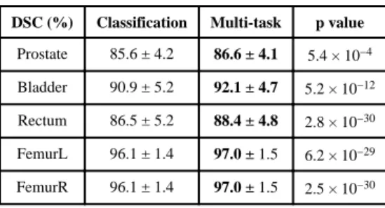
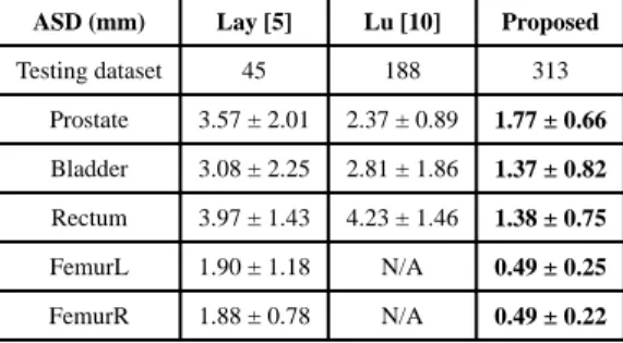
Table. I presents a quantitative comparison between regression random forest and multi-task random forest for guiding deformable segmentation. The p values show that multi-task random forest obtains significantly better results than regression forest on segmenting the prostate, bladder and rectum. For left and right femoral heads, which have high contrast in CT images, both methods perform equally well. Their slight difference is caused by one failure case of regression forest.
Classification Forest—Fig. 9 shows qualitative comparisons of classification map and displacement field between the conventional classification forest and multi-task random forest. Compared to using classification forest to generate the displacement map, it has several advantages to use multi-task random forest.
• In the multi-task random forest, organ classification and displacement regression are mutually beneficial. As we can see from both Fig. 9 (a) and (b), multi-task random forest produces better organ classification maps than conventional classification forest.
• The classification errors can be easily propagated if the displacement field is derived from classification map, especially when there are multiple positive responses in the classification map. Fig. 9 (a) provides a typical example, where mis-classifications in a small region ruin half of the displacement field.
A
uthor Man
uscr
ipt
A
uthor Man
uscr
ipt
A
uthor Man
uscr
ipt
A
uthor Man
uscr
In contrast, if the displacement field is voxel-wisely predicted by multi-task random forest, the mis-predictions are restricted only in local regions and will not be propagated.
• As illustrated in Fig. 10, near the organ boundary, the displacement field predicted by multi-task random forest is often smoother than the one generated from classification map, because binarization of classification map by simple thresholding often produces zigzag organ boundaries.
Table II presents a quantitative comparison between classification forest and multi-task random forest for displacement field prediction. The p values show that multi-task random forest is better than classification forest for displacement field estimation and guiding regression-based deformable segmentation.
E. Iterative Structural Refinement
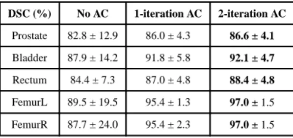
Now we evaluate the contribution of the auto-context model for refining the displacement fields. Table III shows the segmentation accuracies obtained without the auto-context model, with 1 iteration and 2 iterations of the auto-context model, respectively. We can see that the use of auto-context model significantly boosts segmentation accuracies, especially in the first iteration. With an additional iteration, segmentation accuracies further improve. However, the improvement is not as significant as the first one. Considering computational efficiency, we use 2 iterations for structural refinement in this study.
F. Comparison with Conventional Deformable Model
To show the effectiveness of regression-based deformable model, we compare it with conventional classification-based deformable model. Unlike our method, classification-based deformable models require a good initialization to work well. Once the shape model (3D mesh) is well initialized, every vertex on the shape model independently deforms along its inward and outward normal directions to a position with the maximal boundary response. After one-step deformation of all vertices, the entire shape model is often smoothed or regularized by a shape space (e.g., through PCA) before the next round of deformation. These two steps alternate until convergence or reaching the maximum number of iterations.
In this experiment, we use random forest classifier with the same type of Haar-like features and the auto-context model to classify every voxel in a testing image into either “organ” or “background”. The gradient on the obtained organ likelihood map is used as boundary response to guide conventional deformable segmentation. After one-step deformation, we use mesh smoothing and remeshing to regularize the shape model, which is the same as our regression-based deformable model.
We tried two initialization methods for classification-based methods:
• Box-based initialization: The regression-based anatomy detection method [23] is utilized to automatically detect the bounding box of the target organ. Based on the detected box, the mean shape is initialized on the box center and further scaled to fit the box size. After initialization, the shape model deforms as the conventional model.
A
uthor Man
uscr
ipt
A
uthor Man
uscr
ipt
A
uthor Man
uscr
ipt
A
uthor Man
uscr
• Multi-resolution strategy: The mean shape model is initialized to the
classification mass center in the coarsest resolution. Once initialized, the shape model deforms on the organ likelihood map until convergence. After that, the deformed shape model in the coarse resolution is used as an initialization to the next finer resolution. The deformation is hierarchically performed until it meets the finest resolution. We use the same multi-resolution parameters as described in Section IV-C.
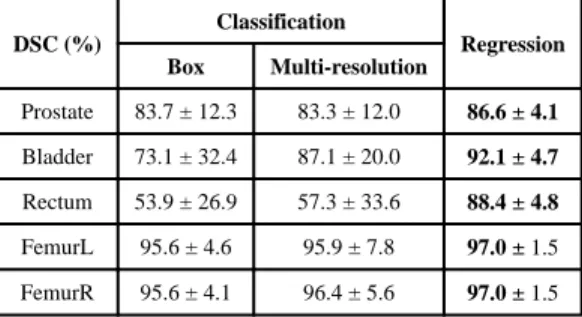
Table IV shows the segmentation accuracies obtained by classification-based deformable models with two initialization strategies, and our regression-based deformable model, respectively. Because the conventional deformable models rely on local search to deform, the parameter of search range is critical to segmentation. Therefore, we manually picked the best search range of each organ for classification-based methods, from 10 to 35 mm with a step size of 5 mm. From the results listed in Table IV, we can see that, for the organs with more rigid shapes and positions, such as the prostate and femoral heads, the conventional classification-based deformable models perform reasonably well, although their
performance is still inferior to ours. However, they fail notably when segmenting organs with highly variable shapes, such as the bladder and rectum.
The main reason for those failures is that initialization is demanded by conventional deformable models. However, a good initialization is often difficult to obtain for flexible organs such as the bladder and rectum. Fig. 11 presents several typical bounding-box-based initializations for illustration. We can see that it is challenging to accurately detect the bounding box of the bladder, due to dramatic changes of bladder size and position across subjects. For the rectum initialization, it is even more challenging. As shown in the right panel of Fig. 11, although the detected bounding boxes (green) are reasonably good, the initialized shapes (green) are still far from the true organ boundaries (red), because of the dissimilarity between the mean rectum shape and individual rectum shapes. The highly variable shapes make bounding-box based initialization less effective in initializing the rectum, compared to other organs, such as the prostate and femoral heads, which have relatively stable shapes. The same challenges also apply to the multi-resolution initialization strategy.
Besides initialization, conventional deformable models still face another challenge when segmenting the rectum. That is the difficulty in determining the search range. Due to tubular structure of the rectum, large search ranges would easily cause mesh folding as vertices of left rectum wall may find high boundary responses from the right rectum wall and vice versa. On the other hand, small search ranges are insufficient to drive the deformable model onto organ boundaries if the shape model is not well initialized. These two contradictory factors make it unfeasible to find a compromised search range. This also explains why the segmentation accuracy of the rectum by the classification-based deformable models is much lower, compared to that of other organs.
In contrast to conventional deformable models, our regression-based deformable model is guided by displacement field, which provides non-local external forces to overcome the sensitivity of deformable models to initialization. Because of this, our method does not
require a model initialization step, which is often critical in most deformable segmentation methods. This characteristic renders our method suitable for segmenting organs, such as the bladder and rectum, which are difficult to initialize. Additionally, the deformation direction and step size of each vertex are optimally predicted during the deformation, according to the underlying image appearance. This feature makes our deformable model appealing to segment organs with complex shapes, such as the rectum, where the conventional
deformation strategies (e.g., normal deformation direction and fixed step size) do not work. All these factors contribute to the success of our regression-based deformable models in CT pelvic organ segmentation.
G. Comparison with Other Segmentation Methods
Finally, we compare our method with existing methods for CT pelvic organ segmentation. The comparisons are separated into two parts. In the first part, we compare our current method with our previous methods [33], [34] on the same dataset. In the second part, we compare our method with works from other groups based on reported performance.
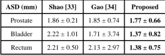
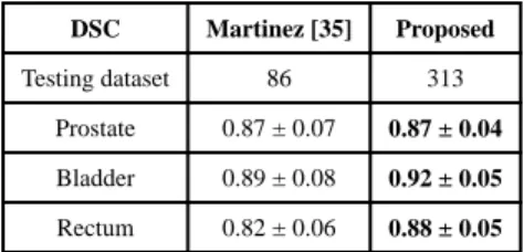
Comparison on the same dataset—Table V and VI quantitatively compares our method with two of our previous methods on the same dataset. Compared to Shao [33], our method achieves a comparable segmentation accuracy of the prostate, i.e., with slightly worse DSC but better ASD. However, in terms of bladder and rectum, the segmentation accuracy is improved a lot, i.e., with mean DSC improved by 6% for the bladder, and 4% for the rectum. The improvement is mainly contributed to the use of regression-based
deformable model, which not only solves the problem of initialization, and also increases the flexibility of deformable models in segmenting organs with complex shape.
Compared to Gao [34], the major improvement is on the rectum segmentation. In Gao [34], the estimated displacement field is used only for initialization. The final segmentation is still obtained by conventional classification-based deformable model. This strategy works reasonably well for the prostate and bladder, whose shapes are elliptic-like. However, it doesn’t work well for the rectum, whose shape is tubular and curvy. By using the estimated displacement field to fully drive deformable model from coarse-level initialization to fine-level segmentation, we obtain a big improvement on the rectum segmentation, i.e., 9% mean DSC increase.
Comparison with other works—Because different methods segment different subsets of the five pelvic organs, and use different metrics to measure their performance, we
separate the comparisons with other works into multiple tables (Tables VII – X). The results show that our method is evaluated on the largest CT dataset, and also achieves the best segmentation accuracy, except that the positive predictive value (PPV) of our method in prostate segmentation is slightly lower than Chen [9]. However, the sensitivity (SEN) of our method is much higher than theirs. Besides, a careful scrutiny on these tables reveals that the improvement of our method over other existing methods is larger on the bladder and rectum than other organs. We think this is mainly because it is difficult for conventional deformable models to segment organs that are difficult to initialize and with highly variable shapes. However, with the introduction of non-local deformation, adaptive deformation direction and
A
uthor Man
uscr
ipt
A
uthor Man
uscr
ipt
A
uthor Man
uscr
ipt
A
uthor Man
uscr
step size, these limitations can be effectively addressed by regression-based deformable models.
It is worth noting that most existing works use either sophisticated methods for model initialization [5], [10], [35], or rely on shape priors [5], [6], [7], [9], [10], [35], [36] to regularize the segmentation. In contrast, our method uses a fairly simple initialization method (i.e., initialize the mean shape model at image center), and does not rely on shape priors (e.g., PCA shape analysis, or sparse shape composition [37]). It is interesting to observe that, even with this setup, our method still results in more accurate outcomes, when compared to previous methods. This demonstrates the robustness of our method to
initialization and the effectiveness of our method in CT pelvic organ segmentation.
V. Conclusion and Discussion
In this paper, we propose to estimate a displacement field for guiding deformable
segmentation. The displacement field is estimated by multi-task random forest, which has shown better performance than conventional random forest in displacement field estimation. To overcome the limitation of independent voxel-wise prediction, we revisit the auto-context model and utilize it to iteratively incorporate the structural information learned from training images. Extensive experiments on a large CT dataset show that the proposed regression-based deformable model is robust to initialization, and achieves better segmentation accuracies than the conventional classification-based deformable models and several other existing segmentation methods for CT pelvic organ segmentation.
Acknowledgments
This work was supported by NIH grants (EB006733, EB008374, EB009634, CA140413).
References
1. American Cancer Society. Cancer facts & figures 2015. 2015
2. Shen D, Lao Z, Zeng J, Zhang W, Sesterhenn IA, Sun L, Moul JW, Herskovits EH, Fichtinger G, Davatzikos C. Optimized prostate biopsy via a statistical atlas of cancer spatial distribution. Medical Image Analysis. 2004; 8(2):139–150. [PubMed: 15063863]
3. Zhan Y, Shen D, Zeng J, Sun L, Fichtinger G, Moul J, Davatzikos C. Targeted prostate biopsy using statistical image analysis. Medical Imaging, IEEE Transactions on. 2007; 26(6):779–788.
4. Foskey M, Davis B, Goyal L, Chang S, Chaney E, Strehl N, Tomei S, Rosenman J, Joshi S. Large deformation three-dimensional image registration in image-guided radiation therapy. Phys Med Biol. 2005; 50(24):5869. [PubMed: 16333161]
5. Lay, N.; Birkbeck, N.; Zhang, J.; Zhou, S. Rapid multi-organ segmentation using context integration and discriminative models. In: Gee, J.; Joshi, S.; Pohl, K.; Wells, W.; Zllei, L., editors. Information Processing in Medical Imaging, ser. Lecture Notes in Computer Science. Vol. 7917. Berlin Heidelberg: Springer; 2013. p. 450-462.
6. Freedman D, Radke RJ, Tao Z, Yongwon J, Lovelock DM, Chen GTY. Model-based segmentation of medical imagery by matching distributions. Medical Imaging, IEEE Transactions on. 2005; 24(3):281–292.
7. Costa MJ, Delingette H, Novellas S, Ayache N. Automatic segmentation of bladder and prostate using coupled 3d deformable models. Med Image Comput Comput Assist Interv. 2007; 10(Pt 1): 252–260. [PubMed: 18051066]
8. Feng Q, Foskey M, Tang S, Chen W, Shen D. Segmenting ct prostate images using population and patient-specific statistics for radiotherapy. 2009:282–285.
9. Chen S, Lovelock DM, Radke RJ. Segmenting the prostate and rectum in ct imagery using anatomical constraints. Medical Image Analysis. 2011; 15(1):1–11. [PubMed: 20634121] 10. Lu, C.; Zheng, Y.; Birkbeck, N.; Zhang, J.; Kohlberger, T.; Tietjen, C.; Boettger, T.; Duncan, J.;
Zhou, S. Precise segmentation of multiple organs in ct volumes using learning-based approach and information theory. In: Ayache, N.; Delingette, H.; Golland, P.; Mori, K., editors. Medical Image Computing and Computer-Assisted Intervention MICCAI 2012, ser. Lecture Notes in Computer Science. Vol. 7511. Berlin Heidelberg: Springer; 2012. p. 462-469.
11. Li W, Liao S, Feng Q, Chen W, Shen D. Learning image context for segmentation of the prostate in ct-guided radiotherapy. Physics in Medicine and Biology. 2012; 57(5):1283–1308. 3. [PubMed: 22343071]
12. Lu, C.; Chelikani, S.; Papademetris, X.; Knisely, JP.; Milosevic, MF.; Chen, Z.; Jaffray, DA.; Staib, LH.; Duncan, JS. An integrated approach to segmentation and nonrigid registration for application in image-guided pelvic radiotherapy. Medical Image Analysis; special Issue on the 2010
Conference on Medical Image Computing and Computer-Assisted Intervention; 2011. p. 772-785. 13. Liao S, Gao Y, Lian J, Shen D. Sparse patch-based label propagation for accurate prostate
localization in ct images. Medical Imaging, IEEE Transactions on. 2013; 32(2):419–434. 14. Moore EM, Magrino TJ, Johnstone PAS. Rectal bleeding after radiation therapy for prostate
cancer: Endoscopic evaluation. Radiology. 2000; 217(1):215–218. pMID: 11012447. [PubMed: 11012447]
15. Hanlon AL, Bruner DW, Peter R, Hanks GE. Quality of life study in prostate cancer patients treated with three-dimensional conformal radiation therapy: Comparing late bowel and bladder quality of life symptoms to that of the normal population. International Journal of Radiation Oncology*Biology*Physics. 2001; 49(1):51–59.
16. Macdonald A, Bissett J. Avascular necrosis of the femoral head in patients with prostate cancer treated with cyproterone acetate and radiotherapy. Clinical Oncology. 2001; 13(2):135–137. [PubMed: 11373877]
17. Tu Z, Bai X. Auto-context and its application to high-level vision tasks and 3d brain image segmentation. IEEE Trans Pattern Anal Mach Intell. 2010; 32(10):1744–1757. [PubMed: 20724753]
18. Gao Y, Zhan Y, Shen D. Incremental learning with selective memory (ilsm): Towards fast prostate localization for image guided radiotherapy. Medical Imaging, IEEE Transactions on. 2014 Feb; 33(2):518–534.
19. Cootes TF, Taylor CJ, Cooper DH, Graham J. Active shape models—their training and application. Comput. Vis. Image Underst. 1995 Jan.61(1):38–59.
20. Zhan Y, Shen D. Deformable segmentation of 3-d ultrasound prostate images using statistical texture matching method. Medical Imaging, IEEE Transactions on. 2006 Mar; 25(3):256–272. 21. Zhang S, Zhan Y, Metaxas DN. Deformable segmentation via sparse representation and dictionary
learning. Medical Image Analysis. 2012; 16(7):1385–1396. [PubMed: 22959839]
22. Gao, Y.; Shen, D. Context-aware anatomical landmark detection: Application to deformable model initialization in prostate ct images. In: Wu, G.; Zhang, D.; Zhou, L., editors. Machine Learning in Medical Imaging, ser. Lecture Notes in Computer Science. Vol. 8679. Springer International Publishing; 2014. p. 165-173.
23. Criminisi A, Robertson D, Konukoglu E, Shotton J, Pathak S, White S, Siddiqui K. Regression forests for efficient anatomy detection and localization in computed tomography scans. Medical Image Analysis (MedIA). 2013
24. Zheng Y, Barbu A, Georgescu B, Scheuering M, Comaniciu D. Four-chamber heart modeling and automatic segmentation for 3-d cardiac ct volumes using marginal space learning and steerable features. Medical Imaging, IEEE Transactions on. 2008 Nov; 27(11):1668–1681.
25. Criminisi A, Shotton J, Konukoglu E. Decision forests: A unified framework for classification, regression, density estimation, manifold learning and semi-supervised learning. Foundations and Trends in Computer Graphics and Vision. 2012; 7(2–3):81–227.
26. Caruana R. Multitask learning. Machine Learning. 1997; 28(1):41–75.
27. Viola P, Jones M. Robust real-time face detection. International Journal of Computer Vision. 2004; 57(2):137–154.
28. Liu J, Udupa J. Oriented active shape models. Medical Imaging, IEEE Transactions on. 2009 Apr; 28(4):571–584.
29. Wang L, Gao Y, Shi F, Li G, Gilmore JH, Lin W, Shen D. Links: Learning-based multi-source integration framework for segmentation of infant brain images. NeuroImage. 2015; 108:160–172. [PubMed: 25541188]
30. Gao Y, Shen D. Collaborative regression-based anatomical landmark detection. Physics in Medicine and Biology. 2015; 60(24):9377. [PubMed: 26579736]
31. Zhang J, Gao Y, Wang L, Tang Z, Xia J, Shen D. Automatic craniomaxillofacial landmark digitization via segmentation-guided partially-joint regression forest model and multi-scale statistical features. Biomedical Engineering, IEEE Transactions on. 2015; PP(99):1–1. 32. Huynh T, Gao Y, Kang J, Wang L, Zhang P, Lian J, Shen D. Estimating ct image from mri data
using structured random forest and auto-context model. Medical Imaging, IEEE Transactions on. 2015; PP(99):1–1.
33. Shao Y, Gao Y, Wang Q, Yang X, Shen D. Locally-constrained boundary regression for
segmentation of prostate and rectum in the planning ct images. Medical Image Analysis. 2015 –. 34. Gao, Y.; Lian, J.; Shen, D. Joint learning of image regressor and classifier for deformable
segmentation of ct pelvic organs. In: Navab, N.; Hornegger, J.; Wells, W.; Frangi, A., editors. Medical Image Computing and Computer-Assisted Intervention MICCAI 2015, ser. Lecture Notes in Computer Science. Vol. 9351. Springer International Publishing; 2015. p. 114-122.
35. Martnez F, Romero E, Dran G, Simon A, Haigron P, de Crevoisier R, Acosta O. Segmentation of pelvic structures for planning ct using a geometrical shape model tuned by a multi-scale edge detector. Physics in Medicine and Biology. 2014; 59(6):1471. [PubMed: 24594798]
36. Rousson, M.; Khamene, A.; Diallo, M.; Celi, J.; Sauer, F. Constrained surface evolutions for prostate and bladder segmentation in ct images. In: Liu, Y.; Jiang, T.; Zhang, C., editors. Computer Vision for Biomedical Image Applications, ser. Lecture Notes in Computer Science. Vol. 3765. Berlin Heidelberg: Springer; 2005. p. 251-260.
37. Zhang S, Zhan Y, Dewan M, Huang J, Metaxas DN, Zhou XS. Towards robust and effective shape modeling: Sparse shape composition. Medical Image Analysis. 2012; 16(1):265–277. [PubMed: 21963296]
A
uthor Man
uscr
ipt
A
uthor Man
uscr
ipt
A
uthor Man
uscr
ipt
A
uthor Man
uscr
Fig. 1.
Typical CT scans and their pelvic organ segmentations. Three columns indicate images from three patients. The first, second, and third rows show an original sagittal CT slice, the same slice overlaid with segmentations, and a 3D view of segmentations of each patient. Red: Prostate; Green: Bladder; Blue: Rectum; Yellow: Left femoral head; Cyan: Right femoral head.
A
uthor Man
uscr
ipt
A
uthor Man
uscr
ipt
A
uthor Man
uscr
ipt
A
uthor Man
uscr
Fig. 2.
The basic flowchart of regression-based deformable model. Yellow contours in the leftmost and rightmost figures indicate the initialized deformable model and the final segmentation, respectively. In the middle two figures, color indicates the magnitude of estimated
displacement. Blue and red indicates small and large magnitudes, respectively. The magnitude increases with the following color ordering: blue, cyan, green, yellow and red. The colder the color is, the smaller the magnitude is.
A
uthor Man
uscr
ipt
A
uthor Man
uscr
ipt
A
uthor Man
uscr
ipt
A
uthor Man
uscr
Fig. 3.
Illustration of displacement regression and organ classification. Red point indicates a query voxel, and the red rectangle is a local patch centered at the query voxel. Colors in the displacement field indicate displacement magnitudes. The colder the color is, the smaller the magnitude is.
A
uthor Man
uscr
ipt
A
uthor Man
uscr
ipt
A
uthor Man
uscr
ipt
A
uthor Man
uscr
Fig. 4.
Left: one-block Haar-like feature. Right: two-block Haar-like feature. Red, green and blue rectangles denote the local patch, the positive block and the negative block, respectively.
A
uthor Man
uscr
ipt
A
uthor Man
uscr
ipt
A
uthor Man
uscr
ipt
A
uthor Man
uscr
Fig. 5.
(a) Flowchart of iterative structural refinement. Red point is a query point. Red rectangle is a local patch of the query point in the CT image, where appearance features are extracted. Purple rectangles are local patches of the query point in the prediction maps, where context features are extracted. (b) Shape refinements by the auto-context model (AC). Upper: Prostate. Lower: Bladder.
A
uthor Man
uscr
ipt
A
uthor Man
uscr
ipt
A
uthor Man
uscr
ipt
A
uthor Man
uscr
Fig. 6.
Schematic diagram of auto-context with n iterations.
A
uthor Man
uscr
ipt
A
uthor Man
uscr
ipt
A
uthor Man
uscr
ipt
A
uthor Man
uscr
Fig. 7.
Qualitative comparison of displacement fields predicted by conventional regression forest and multi-task random forest. The first, second and third rows show two typical cases of the prostate, bladder and rectum, respectively. Red contours are the ground-truth segmentation, manually contoured by radiation oncologists. The segmentation accuracy (DSC) obtained by using each predicted displacement field is shown as a white number in the right bottom of each color-coded image.
A
uthor Man
uscr
ipt
A
uthor Man
uscr
ipt
A
uthor Man
uscr
ipt
A
uthor Man
uscr
Fig. 8.
The sensitivity of segmentation accuracy to the weight w in Eq. 2 (left) and deformation iteration (right).
A
uthor Man
uscr
ipt
A
uthor Man
uscr
ipt
A
uthor Man
uscr
ipt
A
uthor Man
uscr
Fig. 9.
Qualitative comparisons of displacement fields estimated by conventional classification forest and multi-task random forest.
A
uthor Man
uscr
ipt
A
uthor Man
uscr
ipt
A
uthor Man
uscr
ipt
A
uthor Man
uscr
Fig. 10.
Left: displacement field derived from classification map. Right: displacement field estimated by multi-task random forest.
A
uthor Man
uscr
ipt
A
uthor Man
uscr
ipt
A
uthor Man
uscr
ipt
A
uthor Man
uscr
Fig. 11.
Typical cases of bounding-box-based initialization (Left: bladder; Right: rectum). The second row shows the initialized shapes according to the detected bounding boxes in the first row. Red and green contours indicate the ground-truth and the results obtained by anatomy detection, respectively.
A
uthor Man
uscr
ipt
A
uthor Man
uscr
ipt
A
uthor Man
uscr
ipt
A
uthor Man
uscr
A
uthor Man
uscr
ipt
A
uthor Man
uscr
ipt
A
uthor Man
uscr
ipt
A
uthor Man
uscr
ipt
TABLE I
Quantitative comparison of segmentation accuracies (DSC) obtained by regression forest (Regression) and multi-task random forest (Multi-task). Bold numbers indicate the better performance.
DSC (%) Regression Multi-task p value
Prostate 84.0 ± 12.6 86.6 ± 4.1 1.7 × 10⁻⁴
Bladder 90.6 ± 8.6 92.1 ± 4.7 2.7 × 10⁻⁵
Rectum 85.2 ± 6.6 88.4 ± 4.8 1.2 × 10−38