Properties of Shapes Applied to Hippocampi
J¨orn Schulz · Stephen M. Pizer · J.S. Marron · Fred Godtliebsen
November 20, 2013
Abstract This paper presents a novel method to test mean differences of geometrical object properties (GOPs). The method is designed for data whose repre-sentations include both Euclidean and non-Euclidean elements. It is based on advanced statistical analysis methods such as backward means on spheres. We de-velop a suitable permutation test to find global and lo-cal morphologilo-cal differences between two populations based on the GOPs. To demonstrate the sensitivity of the method, an analysis exploring differences between hippocampi of first episode schizophrenics and con-trols is presented. Each hippocampus is represented by a discrete skeletal representation (s-rep). We inves-tigate important model properties using the statistics of populations. These properties are highlighted by the s-rep model that allows accurate capture of the object interior and boundary while, by design, being suit-able for statistical analysis of populations of objects. By supporting non-Euclidean GOPs such as direction vectors, the proposed hypothesis test is novel in the study of morphological shape differences. Suitable dif-ference measures are proposed for each GOP. Both global and local analyses showed statistically signifi-cant differences between the first episode schizophren-ics and controls.
J. Schulz
Department of Mathematics and Statistics, UiT The Arctic University of Norway, Norway Tel.: +47 45696867
E-mail: [email protected]
F. Godtliebsen
Department of Mathematics and Statistics, UiT The Arctic University of Norway, E-mail: [email protected]
Stephen M. Pizer
Department of Computer Science, University of North Car-olina at Chapel Hill (UNC), USA, E-mail: [email protected]
J.S. Marron
Department of Statistics & Operations Research, UNC, USA, E-mail: [email protected]
Keywords Hippocampus·Hypothesis test · Permu-tation test·Principal nested sphere ·Schizophrenia· Skeletal representation
1 Introduction
Statistical analysis of anatomical shape differences has been broadly reported in the literature (e.g., [2,5,10, 15]). In medical settings, the study of morphological changes of human organs and body structures is of great interest. An important subfield in medical imag-ing is to understand neuroanatomical structures of the human brain (e.g., [12,14,42]). Morphological changes of brain structures can provide the physician with information about neuropsychiatric diseases such as Alzheimer’s and schizophrenia. A common interest of medical shape analysis is to test for morphological dif-ferences between healthy and diseased populations. In addition, the study of drug effects is of high interest in epidemiology. Volumetric measurements often can not distinguish between brain structure differences of two populations [45]. Therefore, sophisticated mathe-matical shape models with properties that support an accurate statistical analysis are required.
Shape differences can be quantified by hypothe-sis tests. A statistical hypothehypothe-sis test requires a null hypothesis H0 and an alternative hypothesis H1; a standard null hypothesis assumes no differences be-tween the populations. In this paper, we propose a novel approach for a hypothesis test on geometrical object properties (GOPs) of shapes with application to the hippocampus of the human brain.
method for constructing a hypothesis test based on given difference measures.
We use a discrete skeletal representation, abbrevi-ated as s-rep [36] as a shape model. The amenities of s-reps relative to other shape representations are de-scribed in Section 3. The s-reps are fit to a set of binary images of the hippocampus extracted from a mag-netic resonance imaging (MRI) data set. All skeletal shape models have Euclidean as well as non-Euclidean components. Thus, a hypothesis test based on skeletal models must support the two different types of fea-tures. The approach presented in this paper allows a sensitive hypothesis test between the components of s-reps. By using this approach, local and global shape differences of the hippocampi between schizophrenia and control populations are investigated.
The hypothesis test requiresi)fair correspondence between all skeletal models within a population and across populations, ii) a method to compute means of populations of skeletal models, iii) a test statistic with appropriate distance measures for the Euclidean and non-Euclidean components of the means, iv) a method to calculate a test statistic and the empirical distribution of the test statistic, and v) a procedure to correct for multiple comparison of local and global testing of GOPs.
The paper is presented as follows. The data set for the schizophrenia study describing two shape popu-lations is presented in Section 2. The skeletal model is discussed in Section 3 in addition to required sta-tistical properties for shape analysis of populations. Section 4 introduces the method composite principal nested great spheres (CPNG), which allows statisti-cal analysis of the Euclidean and non-Euclidean com-ponents of skeletal models such as the calculation of means. Section 5 describes the model fitting proce-dure for the two shape populations, which produces the statistical properties required for each model. A permutation test is introduced in Section 6 and spec-ified for skeletal models together with required statis-tics. Finally in Section 7, hypothesis test results of the hippocampus study are reported.
2 Schizophrenia study data set
The data consist of MRI assessments of hippocampi from patients with schizophrenia and a similar set from a healthy control group as described in [28,40]. In the original study, 238 first-episode schizophrenics and 56 controls were enrolled. First-episode schizophrenia patients have not received medical treatment prior to the MRI assessment. The hippocampi were segmented from the aligned MRI scans with an automated atlas based segmentation tool developed at the University of North Carolina [16,28].
Statistical analysis must be performed on either the left or right hippocampus as a combined analysis could bias the result. Accordingly, the left hippocam-pus is evaluated in this paper. Records of the the left hippocampus were not available for 17 patients from the schizophrenia group. Therewith, the data set con-sists of 221 first-episode schizophrenia cases (SG) and 56 control cases (CG) and is represented by binary files which reflect the segmented hippocampi. In the data provided, the hippocampi have been normalized in volume but the original volumes were reported as separate scaling features.
3 Object representation
The representation by a shape model allows calcula-tion of shape statistics of the hippocampus. The type of model, chosen to compare two shape populations, should capture a rich collection of GOPs presented in the data. In addition, small deformations in objects should be reflected by small deformations in the mod-els. Finally, the model should not introduce artificial variation across a population which is not present in the objects themselves.
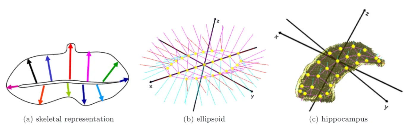
As discussed by [36], a model that fulfills these three properties is an interior-filling s-rep as depicted in Figure 1. Starting with the continuous case, this model and its properties will be discussed in the fol-lowing.
The desired GOPs of the model can be catego-rized into three groups. The first group (G1) should capture locational information of the object bound-ary. The second group (G2) should reflect the local surface curvature by incorporating directional infor-mation into the shape model. The shape model should accurately depict the local orientation of the object. The third group (G3) should describe how the object boundary is connected by the interior in order to re-flect the relationship across the interior of the object. The thickness of an object is one property of the in-terior among others. Skeletal models are designed to obtain these geometric properties.
(a) skeletal representation (b) ellipsoid (c) hippocampus
Fig. 1: Continuous skeletal representation and fitted s-reps. (a) Sectional view of a two-sided skeletal 3D object representation. Colored spokes emanate from the skeletal sheet (which is not medial) to the surface. In the continuous form there is a spoke on each point on the skeletal sheet. (b) Discrete s-rep of a non-deformed 3D ellipsoid. (c) Discrete s-rep of a hippocampus.
of the spokes. The points ofMΩdescribe the inherent symmetry of an object and therewith (G3) above.
Strictly medial representations are limited by the fact that every protruding boundary kink results in additional medial branches. Thus, two versions of the same object with small noise can have drastically dif-ferent medial representations. Skeletal models achieve additional stability by relaxing the medial constraint. Figure 1a visualizes a sectional view of a two-sided skeletal object representation in R3 composed of a skeletal sheet and spokes which emanate from a skele-tal position on the skeletal sheet to the surface. The skeletal sheet is close to midway but is not medial. An exactly medial representation of this object would re-quire the setMΩ to include an additional long branch. Elimination of such branches inMΩ is the goal of the skeletal representation. Figures 1b and 1c will be dis-cussed later.
Stability in the branching structure and stability in the skeletal sheet ensure structural case-by-case stabil-ity of the model and thus good correspondence across the samples in the full data set. The branching con-straint can be tightened for specific classes of objects where the shape is known. For an ellipsoid-like object shape, such as the hippocampus, the constraint of no branching is reasonable and is adopted. Yet, we want to retain as much as possible the medial properties, such as orthogonal spokes to the boundary and ap-proximately equal spoke length on both sides of the skeletal sheet. Therefore, the family of skeletal models is restricted by the class of interior-filling s-reps that are modeled as medial as possible [36].
In addition to the case-by-case stability, we require population stability to avoid artificial variance across a population that is solely an artifact of the individual s-rep fittings; such variance is not connected to the ob-jects themselves. Population stability can be achieved by a re-fitting step of the s-rep to the object using an
estimated shape probability distribution of the popu-lation. The re-fitting step reduces the variance of the s-rep population as described in Section 5. Both case-by-case stability and population stability ensure that the shape models have improved correspondence of both the spokes and the skeletal locations between objects, which will support accurate statistics across a population.
A discrete s-rep, as required for the numerical anal-ysis of slab-shaped objects, consists of a two-sided (folded) sheet of skeletal positions sampled as a grid of atoms, whose skeletal positions are depicted as small spheres in Figures 1b and 1c. On each side of the sheet, there is a spoke, a vector with direction and length on the top and on the bottom connecting the skele-tal sheet to the boundary. Also, for each edge grid point there is an additional spoke vector connecting the skeletal sheet fold to the crest of the slab. The sheet is close to midway consistent to the fixed branch-ing constraint between the two sides of the slab, and the spokes are approximately orthogonal to the object boundary. Each discrete s-rep is described by a feature vector
s= (p1, . . . , pna, r1, . . . , rns, u1, . . . , uns) (1)
withna =next
a +ninta the number of atoms andns=
3next
a + 2ninta is the number of radii and spoke
direc-tions. A slabular s-rep consists of next
a exterior (edge
grid points) andnint
a interior atoms. An interior atom
consists of a skeletal position p ∈ R3, two spoke di-rectionsu ∈S2
and two spoke lengthsr ∈ R+ (top, bottom) whereS2 ={x∈
R3 | kxk = 1} is the unit sphere. An exterior atom consists of a skeletal position
p∈R3, three spoke directionsu∈S2and three spoke lengthsr∈R+ (top, crest, bottom). As a result, the shape space ofs∈R3na×Rns
+ ×(S
2)nsis a product of
Euclidean and non-Euclidean spaces. Each s-rep can also be described in the spaceRns+1×S3na−4×
together with a scaling factorγ∈R+. This representa-tion is derived from a pre-shape space [22] as discussed in Section 4.
Another popular class of modeling 3D objects is a boundary point distribution model (PDM) where a solid object is defined by the positions of the sampled surface points [8,10,24]. In general, normal directions can be attached on the surface points of a PDM but to the best of our knowledge, it has not been used in practice. In addition, deformation-of-atlas models are well known, wherein the shape changes of an object in images are modeled by the deformations of a template image [34,38]. Such models can capture the local ori-entation of an object. Nevertheless, both approaches are less suitable for shape statistics of populations by the lack of the interior description of an object.
We restrict our analysis to discrete slabular s-reps which are organized into a (3×8) grid of skeletal posi-tions, i.e., each s-rep consists of 24 atoms. The choice of the grid size defines how exactly the binary images can be described by the s-rep model. We have chosen a grid of 3×8 atoms as a trade-off between captur-ing important object features, avoidcaptur-ing an overfittcaptur-ing and keeping the dimension of the shape space low. A hippocampus example with bumps that are not tightly described by a (3×8) grid is visualized in Section 1.1 of the Supplementary Material. However, we do not look at individual s-reps that may not be perfectly correct but rather at differences between groups which are not biased versus the other.
4 CPNG analysis
A hypothesis test on mean differences requires a me-thod to calculate means from populations of shape models. The method should incorporate all geomet-rical components of such models. We have presented in Section 3 an s-rep as a suitable model with Eu-clidean components and components which live on spheres. This section will discuss an approach to pro-duce means, in addition to shape distributions of pop-ulations of s-reps.
First of all, we need to understand the shape space of a discrete s-rep to apply a proper statistical analy-sis. Each discrete s-rep is described by a feature vector s∈R3na×Rns
+ ×(S 2
)nsas defined in (1), and lives in a
product of Euclidean and non-Euclidean spaces. Each element of s corresponds across the population. The points Xp = (p1, . . . , pna)
′
∈ R3na form an (na ×3)
matrix and a PDM that can be centered and normal-ized at the origin by ZH = HXp/kHXpk with H a Helmert sub-matrix which removes the origin [10,22].
H is an ((na−1)×na) matrix with rowi−1 defined by the vector
(H)i−1= (di, . . . , di,−idi,0, . . . ,0)
with di = (i(i+ 1))−1
2, i = 2, . . . , na where di is re-peated i-times. ZH is called a pre-shape with infor-mation of location and scale removed. Therewith, the Cartesian product ofpi∈R3, i= 1, . . . , na can be de-scribed by the pre-shape ZH and by a scaling term
γ=kHXpk. The pre-shapeZH lives on the (3na−4) dimensional unit sphereS3na−4⊂
R3na−3. Each spoke direction ui, i= 1, . . . , nsofslives on the unit sphere
S2. The radii ri ∈
R+, i = 1, . . . , ns and scale factor
γ ∈ R+ are log-transformed to the Euclidean space
R. Thus, a discrete s-rep s can be described in the shape space Rns+1 ×S3na−4 ×(S2)ns composed of
several spheres and a real space. Jung et al. [20] and Pizer et al. [36] have proposed a method to analyze a population of s-reps that are living in such an ab-stract space. This method is calledcomposite principal
nested spheres (CPNS) and will be discussed in the
following.
Suppose we have a population ofN s-reps. In order to analyze the covariance structure of such a popula-tion, we have to find a common coordinate system. CPNS consists of two main parts. First, the spherical parts are analyzed byprincipal nested spheres (PNS) [18,19], which analyzes data on spheres in decreas-ing dimension, i.e., usdecreas-ing abackward view. Therewith, the pre-shape ZHj and eachuij can be mapped to a Euclidean space with j = 1, . . . , N. Second, the Eu-clideanized variables are concatenated with the logri
and logγto give a matrixZcompand an array of scale factors to make all variables commensurate as dis-cussed in detail in [36]. Finally, the structure of the co-variance is investigated from the scaled matrixZcomp. PNS is a novel method to estimate the joint probabil-ity distribution of data on ad-dimensional sphereSd
by a backward view along the dimensions. The back-ward view allows dealing with one dimension at a time and thus produces better probability distributions.
In Euclidean space, the forward and backward ap-proaches to principal component analysis (PCA) are equivalent, which is not true in general non-Euclidean spaces, such as thed-dimensional unit sphereSd. Da-mon and Marron [9] have studied generalizations (e.g., PNS) of PCA across a variety of contexts, and have shown that backwards is generally more amenable to analysis, because it is equivalent to a simple adding of constraints.
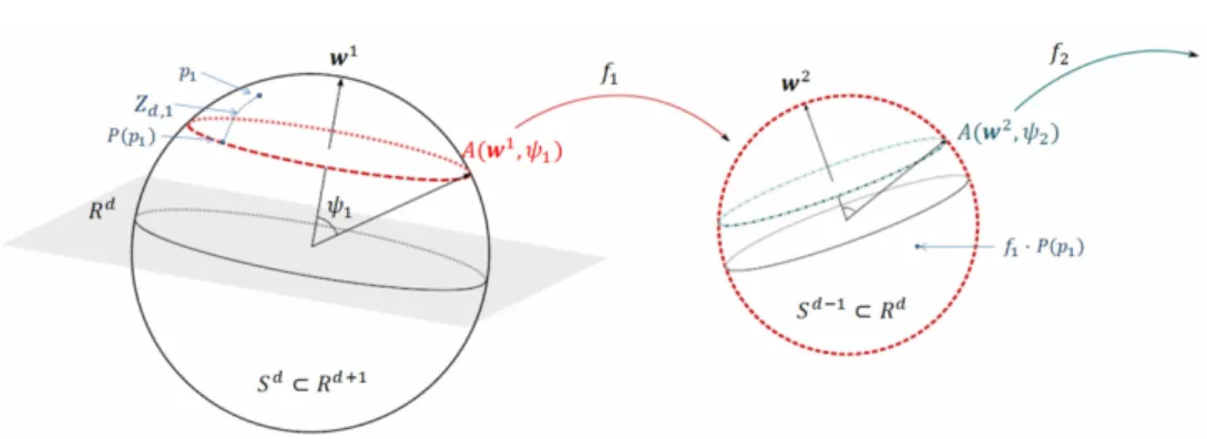
PNS is a fully backward approach that fits the best lower dimensional subsphere in each dimension start-ing with Sd. The subsphere can be great (a sphere
with radius 1) or small (less than 1). Figure 2 visu-alizes the method which takes into account variation along small circles (non-geodesic variations) as well as variation along geodesics. Thus, the decomposition is non-geodesic. Each subsphereA(wl, ψl) ofSd−l+1is defined by an axis (polar position)wlwith latitude
Fig. 2: Backwards PNS by computation of the nearest lower dimensional subsphere. In addition, the projection
P(p1) of a data pointp1 with scoreZd,1 on the subsphereA(w1, psi1) is depicted.
A(wd, ψd) is a circle. The Fr´echet mean [13,21] on the
remaining 1-dimensional subsphere can be seen as the best-fitting 0-dimensional subsphere (a point) of the data. Finally, this mean is projected back toSd
result-ing in a backward Fr´echet mean.
CPNS has been shown to be powerful in the anal-ysis of a single s-rep population. In this study, our hypothesis test of local or global shape differences in-volves the comparison of two or more CPNS statistics, which is facilitated by stable statistics and correspon-dence between populations, using a common coordi-nate system. In fact, PNS is a non-geodesic method which fits small and great subspheres. The fitting of small spheres has advantages in describing the amount of data variation inside a population with fewer princi-pal components, but two or more populations can have different decompositions into small and great spheres, which introduce additional variation across the popu-lations, e.g., reflected by a larger variation between CPNS means of several populations. Therefore, all CPNS analyses in this paper are constrained by fit-ting principal nested great spheres, called PNG and CPNG respectively. Therewith, we avoid additional variation, ensure correspondence and a common coor-dinate system across several populations. A prelimi-nary simulation study on permuted populations of s-reps confirmed the improvements of CPNG compared to CPNS. Notice, CPNG is identical to [17] in the two dimensional case. We are leaving a commensurate CPNS analysis for populations using small spheres for future work and discuss a possible approach in Sec-tion 1.2 of the Supplementary Material.
5 Model fitting
The application of the proposed hypothesis test to the hippocampi study, introduced in Section 2, requires a procedure to generate s-rep fittings with statistical object and population properties as discussed in Sec-tion 3. This secSec-tion will introduce such a procedure.
Assume we have a set of binary images and a set of corresponding signed distance images. The distance images are used during the fitting process as the tar-get data to which reference models are fitted. Follow-ing [36], the fittFollow-ing procedure can be described with 5 consecutive steps: initial alignment, atom stage, spoke stage, CPNG stage and the final spoke stage.
Initial alignment:A reference s-rep is translated, ro-tated and scaled into the space of distance images by matching of moments to the interior.
Atom stage: The atom stage defines the geometry of the object and accordingly, the case-by-case stabil-ity. Each atom, i.e., each skeletal grid point and its set of spokes are fit one by one with multiple itera-tions through these atoms. For each atom, an objec-tive function is optimized [36]. The objecobjec-tive function reflects the goodness of the fit and is calculated by a weighted sum of different optimization criteria. The function penalizes factors which are making the s-rep structurally improper, such as irregularity in the grid and crossing of adjacent spokes. In addition, it penal-izes the spoke ends deviating from the object bound-ary and their directions deviating from the boundbound-ary normal (both implied by the input distance image). The spokes are further penalized from failing to match the geometry of the crest implied by the distance im-age. The penalties are summed over spokes which are interpolated from the original s-rep.
Spoke stage: The spoke stage optimizes the spoke lengths to match the object boundary more closely. The skeletal grid points and the resulting geometry of the s-rep will not be changed during this stage. The atom and spoke stage provide appropriate s-rep fit-tings to the data with case-by-case stability.
but also yields eigenmodes and modes of variation [18]. Consequently, any s-rep can be expressed by the score of the eigenmodes in the CPNG space. Hence, corre-spondence across a population is achieved by initial-ization of each fitting with the CPNG mean s-rep and by restricting the shape space to the CPNG space. In addition, s-rep candidates from the CPNG space are penalized by the Mahalanobis distance between the candidate and the CPNG mean. As a result improved correspondence is achieved.
Final spoke stage:The final spoke stage adjusts the spokes of the CPNG stage fits to match closely the ob-ject boundary. Consequently, s-reps can be generated which are not an element of the CPNG space.
The first three stages form a preliminary stage in the fitting procedure. The fitting stages are imple-mented in a software called Pablo, developed at the University of North Carolina. The program is avail-able at [32].
6 Multiple hypothesis testing
A sensitive hypothesis test is useful for the quantifica-tion of shape differences, both to compare populaquantifica-tions globally and locally. The introduction of a suitable shape model in Section 3, a method to calculate means from populations in Section 4 and a procedure to gen-erate s-rep fittings in Section 5 provide us with tools to generate models and means that contain the desired properties for a sensitive hypothesis test. An impor-tant challenge is that the geometric object elements of each model are spatially correlated. Furthermore, a suitable hypothesis test should correct for multiple comparisons.
6.1 An overview of multiple comparison corrections
The problem of false positives with multiple statistical tests is well recognized. Statistical shape analysis must deal with a large number of hypotheses, each derived from a GOP element, for example of the s-rep. Two common categories of multiple comparison correction are familywise error rate (FWER) and false discovery rate (FDR) [3]. Let V be the number of rejected hy-potheses when the null is true (type 1 error), and S
the number rejected hypotheses when the null is false. The FWER is defined as the probability of at least one type 1 error by P(V ≥1). The FDR is defined as the expected proportion of type 1 errors among the total number of rejected hypotheses by E(V /(S+V) with V /(S+V) = 0 if (S+V) = 0. There are sev-eral approaches to control FWER and FDR. A com-monly used one is the Bonferroni correction. Another approach is using typical wavelet coefficient selection
methods [1,6,44]. In addition, variable selection based on threshold random field theory (RFT) have been used [7,23,33]. Permutation tests allow multiple com-parison correction by estimating the empirical null-distribution and the covariance structure of the test statistics [30,35,43]. This paper uses multiple compar-ison correction by FWER.
The Bonferroni correction has several major draw-backs; the Bonferroni threshold can be conservative if the GOPs are dependent of each other. In partic-ular, spatial autocorrelations result in fewer effective variables. Spatial correlation can be expected between neighbor spokes and skeletal positions of an s-rep. In addition, the Bonferroni correction reduces the power of a test as the probability of false negatives increases, because it controls only the probability of false pos-itives. RFT requires strong assumptions such as the same parametric distribution at each spatial location (e.g., multivariate Gaussian), sufficient smoothness as well as stationarity. The assumption of a parametric distribution can not be fulfilled in case of an s-rep model, and the assumption of stationarity can also be doubtful.
Permutation tests have advantages over the ap-proaches above that make them particularly suitable for s-reps. S-reps are defined on a product of Euclidean and non-Euclidean spaces with unknown probability distributions of the geometric object elements. In con-trast to standard parametric methods such as Bonfer-roni and RFT, a permutation test is a non-parametric approach using the data to estimate the sampling dis-tribution of the test statistic under the null-hypothesis
H0. Permutation tests are also adaptive to underlying correlation patterns in the data.
A minimal assumption of permutation testing is the exchangeability underH0such as identical distri-butions of populations 1 and 2. The underlying idea of a permutation test is that any permutation of the observations has the same probability to occur under the assumptionH0. Given the permuted populations, a common test statistic measures differences between population means. The test statistic may calculate fea-ture by feafea-ture differences or combine feafea-tures to mea-sure differences between GOPs. The permuted pop-ulations can be used to estimate the distribution of the test statistic as well as to estimate the correlation structure.
6.2 A permutation test for s-reps
Suppose we have two populations of s-reps described by a set ˜A1 ={˜s11, . . . ,˜s1N1} of N1 s-reps and a set
˜
A2 ={˜s21, . . . ,˜s2N2} ofN2 s-reps with ˜sil as defined
The permutation test for populations of s-reps can be divided into four steps.
First, observed and permuted population CPNG means are generated as described in Section 6.2.2. Second, appropriate Euclidean or non-Euclidean GOP differences are calculated between the means of the observed populations ˜A1 and ˜A2, and between the means of corresponding permuted populations as de-scribed in Sections 6.2.3 and 6.2.4. Third, p-values are calculated for each GOP difference as described in Section 6.2.5. Each of these p-value is uniformly distributed and mapped by probability integral trans-formations to standard normal distributed variables. Hence, the GOPs can be mapped from a non-linear to a linear space with the same coordinate system for each GOP. Finally, the covariance matrix of these standard normal distributed variables is estimated, in order to incorporate the true multivariate nature of the data and the correlation between the GOPs as de-scribed in Section 6.2.6. As a result, the partial tests of the GOPs can be combined into a single summary statistic by the Mahalanobis distance. In addition, a feature-by-feature test can be constructed as described in Section 6.2.7.
6.2.1 Pre-processing
In a first pre-processing step, global translational and rotational variations should be removed from all s-reps in order to analyze only shape variations. To make the alignment unbiased with respect to the population, the overall backwards CPNG mean ˜µ is estimated from the set union
˜
A= ˜A1
[ ˜
A2={˜s11, . . . ,˜s1N1,˜s21, . . . ,˜s2N2}.
The CPNG mean ˜µ is translationally aligned by the subtraction of the mean of the locational components. In addition, the eigenvectors of the second moments about the center of the skeletal positions yields a ro-tational alignment to the x,y andz-axis. The trans-lationally and rotationally aligned CPNG mean ˜µ is called µ. Afterwards, each s-rep ˜s∈ A˜ is translated, rotated and scaled toµby standard Procrustes align-ment (see [10]) based on the hub-positions of each s-rep. For each aligned s-reps, the scaling factorτ ∈R+ is kept as a variable. The global translation and rota-tion informarota-tion is not considered of interest in the shape analysis of hippocampi. Moreover, we have cho-sen to use features which can be understood by the user (e.g., physicians). Therefore, the skeletal posi-tions are considered in R3na instead on S3na−4 as in Section 4. Thus, each aligned s-rep is described by a feature vector t = (τ,s), where t contains n = 1 +na+ 2ns features and is an element of the shape spaceR3na×Rns+1
+ ×(S
2)ns. SetA
1={t11, . . . ,t1N1}, A2={t21, . . . ,t2N2}and A=A1
S
A2.
6.2.2 Generation of observed and permuted sample means
First, a method to calculate means for the observed and permuted samples of the two populations is re-quired in order to create a hypothesis test of mean differences.
Observed sample means.For each set Ai,i= 1,2 the observed sample mean is ˆµi = (¯τi,µi¯ ) ∈ R3na× Rns+1
+ ×(S 2
)ns. The component ¯µi is a CPNG
back-wards mean as described in Section 4. The mean scal-ing factor ¯τi ∈R+ is computed as a geometric mean (which is natural for scaling factors) by
¯
τi = exp
1
Ni Ni
X
j=1
log(τij)
, i= 1,2. (2)
In fact, the CPNG backwards mean ¯µiconsists ofns+ 1 PNG backwards means, one for the skeletal position andnsfor the spoke directions, andnsmeans for the spoke lengths respective to (2).
Permuted sample means.The number of all possi-ble permutations of the index setI={1, . . . , N1+N2} is
N
1+N2
N1
=(N1+N2)!
N1!N2! .
Random sample sets Il, l = 1, . . . , P of P = 30,000 permutations of the index set I were generated, a number comparable to the suggested number in [11] and [26]. Larger numbers of permutations increase the accuracy of the p-values but require more computa-tion time. The permutacomputa-tion group A1l ⊂A contains
all s-reps indexed by the first N1 indices of Il. The group A2l = A\A1l contains the remaining N2 s-reps. For each permutationIl the means ˆνil, i= 1,2 are estimated by ˆν1l = (¯κ1l,ν¯1l) for the group A1,
ˆ
ν2l = (¯κ2l,ν¯2l) for the group A2. ¯νil is estimated by
the CPNG backwards mean and ¯κil is the mean scal-ing factor of the correspondscal-ing permutation respective to (2).
6.2.3 Test statistics
Equality of distributions between populationsA1 and
A2 can be tested by a nonparametric combination of a finite number of dependentpartial tests as proposed in Pesarin [35]. The global null hypothesis is given by
H0:{A1
d
=A2}, where
d
= denotes the equality in dis-tribution. LetH1be the global alternative hypothesis. In general, the test requires the definition of astatistic
T in testing a null hypothesis. A natural test statistic is
where ˆµ1 and ˆµ2 are the observed sample means as defined in Section 6.2.2 andd is a difference measure on the nonlinear manifold describing the GOPs. The test statisticT consists ofK different partial tests de-pending on the difference measure. Thus, the global null hypothesis can be written in terms of K sub-hypotheses H0 : {TKk=1H0k} and the alternative as H1 : {SKk=1H1k}. Usually, the dependence relation
among partial tests are unknown even though they are functions of the same data. Pesarin [35] has shown that a suitable combining function (described in Sec-tion 6.2.6) will produce an unbiased test for the global hypothesis H0 against H1 if all partial tests are as-sumed to be marginally unbiased, consistent and sig-nificant for large values. The partial tests Tk, k = 1, . . . , K are defined by the partial difference mea-sures. Therewith, a hypothesis test for identical sta-tistical distribution of two s-rep populations is given by mean differences,
H0 :{µ1=µ2}versusH1 : {µ1> µ2} (4)
for a one-sided test in case the difference measures are unsigned and
H0 :{µ1=µ2}versusH1 : {µ16=µ2} (5)
for a two-sided test in case of signed differences. The hypothesisH0will be rejected if the probabil-ity of observingT(A1, A2) underH0 from the empir-ical distribution is smaller than a chosen significance level α; otherwise we do not reject. The significance level describes the probability of type 1 error, i.e.,H0 is wrongly rejected. Alternatively, the type 2 error oc-curs when H0 is not rejected but it is in fact false.
6.2.4 Difference measures
This section defines a signed difference measured2for the test statistic (3). An alternative unsigned differ-ence measured1
is defined in Section 1.3 of the Sup-plementary Material. Suppose we have two s-reps
ti= (τi, pi1, . . . , pina, ri1, . . . , rins, ui1, . . . , uins) ′
,
i = 1,2 with the skeletal positions pij,∈ R3 and the scale factors log(τi),log(rij) ∈Ras Euclidean GOPs and the spoke directions uij ∈ S2 as non-Euclidean GOPs. Thus, a suitable difference measure is required as defined in the following.
The measured2 is a vector of differences
d2
(t1,t2) := (d1(τ1, τ2),
d2(p11, p21), . . . , d2(p1na, p2na),
d3(r11, r21), . . . , d3(r1ns, r2ns),
d4(u11, u21), . . . , d4(u1ns, u2ns)) ′
(6)
with appropriate partial difference measures: d1 for the scaling factors τi, d2 for the positions pik, d3 for the spoke lengths rij and d4 for the spoke directions
uij withi= 1,2,k= 1, . . . , na andj = 1, . . . , nsby
d1(τ1, τ2) = log(τ2)−log(τ1),
d2(p1k, p2k) =p2k−p1k,
d3(r1j, r2j) = log(r2j)−log(r1j), d4(u1j, u2j) =dgs(u1j, u2j).
The partial difference measuredgsis defined by longi-tude and latilongi-tude differences of the spoke directions (u1j, u2j) using a normalization by the shift of the
geodesic mean as explained in the next paragraph. The components of
d2
: (R3na×Rns+1
+ ×(S 2
)ns)×
(R3na×Rns+1
+ ×(S 2
)ns)−→R3na+3ns+1
are not metrics because they can take on negative val-ues.
Shift by the geodesic mean.The spoke directions (u1j, u2j)∈S2×S2can be mapped by spherical
para-metrization to latitudesφ1j, φ2jand longitudesθ1j, θ2j
in the base coordinate system of all aligned hippo-campi. The spherical mapping can be defined by
φij(uij) = atan2(uij3, q
u2
ij1+u 2
ij2),
θij(uij) = atan2(u2
ij2, u 2
ij1),
with φij ∈ [−π/2, π/2] and θij ∈ (−π, π]; the two-argument function atan2(x2, x1)∈(−π, π] is the sign-ed angle between two vectorse1= (1,0)′and (x1, x2)′ ∈R2. The longitudeφis measured from the x-y plane. The spherical mapping is not uniquely defined in general. Furthermore, it does not establish an appro-priate correspondence. Two points close to the equator with identical geodesic distance as two points close to the north pole have different latitude and longi-tude differences, and are therefore not commensurate. For that reason, longitude and latitude pair differ-ences will be normalized by shifting the geodesic mean of (u1j, u2j) along its meridian to the equator by a
rotation about an axis c ∈ S2
with rotation angle
ψ ∈ [0, π/2). Then, the directions (u1j, u2j) are
ro-tated along small circles on the sphere about the same axis c with the same rotation angle ψ towards the equator.
In more detail, consider a pair (u1j, u2j) of spoke
directions on S2 with northpole Np = (0,0,1)′
. At first, find its geodesic mean by
µg(u1j, u2j) = u
1j+u2j
ku1j+u2jk.
We assume acos(|µ′
gNp|))>1e−3; otherwise choose
R1(c, ψ), the rotation ofµg along its meridian to the equator is ˜µg=R1µg with
R1(c, ψ) =I3+ sinψ[c]×+ (1−cosψ)(cc ′
−I3), (7)
whereI3is the three-dimensional unit matrix and [c]×
is the cross product matrix satisfying [c]×v=c×vfor
any v∈R3. To avoid discontinuity problems between −π and π for θij, let R2 be the rotation matrix as defined by (7) that rotates ˜µg towards (1,0,0)′
, i.e.,
R2µg˜ = (1,0,0)
′
. Now, shift each pair (u1j, u2j) by
applying ˜u1j =R2R1u1j and ˜u2j =R2R1u2j. Finally,
we calculate the latitudes φ1j(˜u1j), φ2j(˜u2j) and
lon-gitudesθ1j(˜u1j), θ2j(˜u2j) and define the differences of
the transported spoke directions by the delta latitude
∆φj=φ2j−φ1j and delta longitude∆θj =θ2j−θ1j.
Therewith, the difference measure dgs is defined by
dgs(u1j, u2j) := (∆φj, ∆θj).
6.2.5 Mapping of GOP differences to standard normally distributed variables
Suppose we have the test statistic T0 := T(A1, A2) of the underlying observed sample. The idea is to esti-mate the sampling distribution of the statisticT0from test statistics of the permuted samples
Tl:=T(A1l, A2l), l= 1, . . . , P.
The test statistic measures the GOP differences in dif-ferent units. The vectorTl= (Tl1, . . . , TlK) containsK partial tests, whereKis the number of components of the difference measured2. The elements of the vector
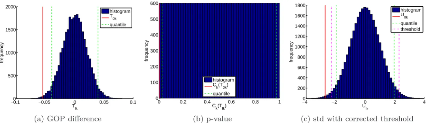
Tl are not commensurate as required for the estima-tion of the covariance structure. Thus, the GOP differ-ences must be normalized and mapped to a common coordinate system in a way that preserves the multi-variate dependence structure between the GOPs. The procedure is explained in the following and depicted in Figure 3 on the basis of a selected GOP using dis-tance measure d2
. The figure is discussed further in the text.
Calculating p-values for GOP differences. Af-ter the calculation of Tl, we estimate for each GOP difference k= 1, . . . , K the empirical cumulative dis-tribution function (CDF) by
Ck(Tlk) = 1
P P
X
l′=1
I(Tl′k, Tlk)
withI(Tl′k, Tlk) =
1 : Tl′k≤Tlk,
0 : otherwise.
Respectively, we can calculate Ck(T0k).
Mapping of p-values to N(0,1). By construction the p-values have a uniform distribution. Thus, the GOP differences can be represented as
Ulk =Φ−1˜
Ck(Tlk), (8)
whereΦ−1 is the inverse standard Gaussian CDF,
˜
Ck(Tlk) =sc−2
sc Ck(Tlk) +
1
sc,
k= 1, . . . , K, l = 1, . . . , P andsc is a scaling factor. The inverse standard Gaussian CDF requires values greater than 0 or less than 1; otherwise Ulk = ±∞. Therefore, all p-values are scaled by ˜Ck(Tlk) withsc= 10000. Simulations have shown numerical instabilities for larger values ofsc. The marginal distribution ofUlk
is standard Gaussian for everyk, i.e,Ulk∼ N(0,1). Using the estimated inverse empirical CDFCk, the observed GOP differencesT0k are mapped toU0k,
re-spectively.
6.2.6 Global test with multivariate comparisons correction
Given Ulk ∼ N(0,1), the K×K covariance matrix
ΣU of theP×KmatrixU = (U1, . . . , UP)′ withUl= (Ul1, . . . , UlK),l= 1, . . . , P is estimated by
ˆ
ΣU = 1
K−1U
′
U.
A corrected test statistic is then given by the Maha-lanobis distances
M0=U
′
0Σˆ
−1
U U0, Ml=U
′
lΣˆ
−1
U Ul, l= 1, . . . , P,
which defines a suitable combining function [35, Sec-tion 6.2.4] that includes the GOP correlaSec-tion struc-ture. The sampling distribution of the final test statis-tic under the null-hypothesis H0 can be estimated fromMl by an empirical CDF. The probability of ob-servingM0underH0from the empirical null-distribu-tion is given by
p(M0) = 1
P P
X
l=1
H(Ml, M0), (9)
withH(Ml, M0) =
1 : Ml≥M0, 0 : Ml< M0.
−0.10 −0.05 0 0.05 0.1 500
1000 1500 2000
T lk
frequency
histogram T
0k quantile
(a) GOP difference
0 0.2 0.4 0.6 0.8 1
0 100 200 300 400 500 600
C k(Tlk)
frequency
histogram C
k(T0k) quantile
(b) p-value
−40 −2 0 2 4
200 400 600 800 1000 1200 1400 1600 1800
U lk
frequency
histogram U
0k quantile threshold
(c) std with corrected threshold
Fig. 3: Mapping of GOP differences to standard normally distributed variables using the example of a skeletal z-position (k= 3) with distance measured2. The 2.5% and 97.5% quantiles are visualized in each plot. (a) GOP differences Tlk of the permuted samples with l = 1, . . . ,30,000 and T0k of the underlying observed sample.
(b) Calculated p-valuesCk(Tlk) andCk(T0k) using the empirical cumulative distribution function. (c) Standard
normal distributed variablesUlk andU0k. The dotted-dashed line depict the corrected thresholdλfor the GOP
as described in Section 6.2.7.
6.2.7 Feature-by-feature test with multivariate comparisons correction
The global shape analysis in the previous section can not indicate local shape differences, which motivates the introduction of an FWER threshold correction for a feature-by-feature test. The permutation test ap-proach on each variable Tlk yields an empirical dis-tribution Ck, dependent standard Gaussian variables
Ulk and the empirical covariance matrix ˆΣU. As a re-sult,Ul= (Ul1, . . . , UlK) is approximately distributed as NK(0,ΣUˆ ), where NK is a multivariate Gaussian
distribution with mean 0, covariance ˆΣU and density functionψ such that each marginal isUlk∼ N(0,1).
Because each random variableUlkis standard Gaus-sian, the threshold for each standard Gaussian variable should be the same. Thus, given a significance levelα, we wish to find the thresholdλsuch that
P(Ul1< λ, . . . , UlK < λ) = 1−
α
2.
The function P is a multiple integral from −∞to λ
in each variable ofUl∼ NK(0,ΣUˆ ) and can be
under-stood as a function g(λ) of the single variableλ. The functiong(λ) is monotonic increasing with asymptotes at 0 and 1. The numerical calculation of the p-values is based on the approximation over an appropriate in-terval ofλ. Recall thatλ≥λcorr with
λcorr=Φ−1 1−α
2
is the threshold for a single standard Gaussian vari-able. Letl∈ {1, . . . , P} be fixed. The thresholdλcorr
is applicable if all U·k are perfectly correlated.
Fur-thermore, we know thatλ≤λindepwith
λindep=Φ−1
1−α
2
1/K
because the thresholdλindepis applicable if allU·k are
independent. The desired level 1−α/2 will be rather near 1. Thus, the functiong(λ) will be concave down-ward in the interval [λcorr, λindep].
The valuesg(λcorr) andg(λindep) can be estimated from a large number NSamp of random samplesYn ∼ NK(0,ΣUˆ ) withn= 1, . . . , NSamp by
ˆ
g(λ) =
PNSamp
n=1 Iλ(ψ(yn1, . . . , ynK))
PNSamp
n=1 ψ(yn1, . . . , ynK)
with Iλ(ψ(yn)) =
ψ(yn) : ψ(yn)< λ,
0 : otherwise,
andyn = (yn1, . . . , ynK). We have chosen a number of
NSamp = 200,000 samples.
The computation ofg(λindep) requires the compar-ison ofyn values only for those identified as not in the accepted subset for the smaller valueλcorrand adding into the accumulated sum for the newly accepted sam-ples. Finally, the standard regula falsi method can be used to iteratively solve the equation g(λ) = 1−α/2 with initial evaluationsg(λcorr) andg(λindep).
The dashed-dotted line (labeled as “threshold”) in Figure 3c shows the correctedλfor a selected GOP.
7 Results
7.1 Fitting of s-reps to hippocampi
and spoke stage were produced as described in Sec-tion 5. This preliminary stage is described in detail in Section 1.4 of the Supplementary Material. In order to control the manual work during the preliminary stage, we considered only the first 96 of 221 cases of SG as discussed in the Supplementary Material. Let ˜A1 be the set of 96 preliminary fits for SG and ˜A2be the set of 56 preliminary fits for CG. All preliminary fits were translated and rotated to the CPNG mean of the set union ˜A1∪A˜2by standard Procrustes alignment [10] in order to remove global variation from the preliminary fits. Let ¯A1 be the set of 96 aligned SG preliminary fits and ¯A2 the set of 56 aligned CG preliminary fits. Finally, CPNG statistics were calculated for the s-rep populations as described in Sections 4 and 5.
A challenging question is the appropriate estima-tion of the shape distribuestima-tions of both populaestima-tions (SG and CG) during the CPNG stage. An option is to cal-culate the CPNG statistic of each population ( ¯A1and
¯
A2), resulting in two means and shape distributions. Another option is to calculate the CPNG statistic of the pooled population ( ¯A1∪A¯2), resulting in a single mean and shape distribution. The use of two individ-ual shape distributions result in independent fittings between the two populations. On the other hand, the fittings should not be biased and have good correspon-dence between the populations, which is provided by a pooled shape distribution. A pooled CPNG statistic also removes possible bias from the manual adjust-ments during the preliminary stage.
The final fitting results obtained from two separate shape distributions showed extraordinary high separa-tion properties and indicated a large bias. Thus, the main focus was the analysis of fittings using a pooled CPNG statistic from ¯A1∪A¯2. In addition, we have generated a second group of final fittings derived from CPNG stages using a pooled shape distribution, two individual shape distributions and two individual in-terchanged shape distributions. The second group is a compromise between independence and a small bias, and is discussed in Section 3 of the Supplementary Material.
Each CPNG statistic contains a backward mean, the eigenmodes and the corresponding CPNG scores. Figure 4 shows the explained amount of variation by the first 25 eigenmodes for the aligned preliminary fittings after atom and spokes stages (1st fittings), i.e., for ¯A1 (subset of SG), ¯A2 (CG) and ¯A1 ∪A¯2. The number of eigenmodes was selected to describe more than 75% of the total cumulative variance. This number compromises on capturing enough shape vari-ation while limiting the shape space in order to avoid overfitting. Accordingly, the first 21 eigenmodes of the pooled shape distribution were selected for the CPNG stage describing 75.2% total variance. 18 eigenmodes are required to describe 75.3% of the total cumulative
variance of ¯A1, and 15 eigenmodes to describe 75.7% for ¯A2.
In the CPNG stage, the obtained backward mean of ¯A1∪A¯2was translationally and rotationally aligned to the 221 SG cases and the 56 CG cases. An ad-ditional scaling of the means would bias the CPNG statistic because the principal components already con-tain size information. Afterwards, the aligned means were optimized inside the CPNG shape space and un-der the penalty of a Mahalanobis distance match term. A high penalty term leads to better correspondence between cases but to less accurate fits. An appropri-ate penalty term was chosen by a simulation study, the report of which is omitted. At the end, the final spoke stage was performed to ensure that the spoke directions match the boundary.
Figure 4 also shows CPNG analyses for the ob-tained 2nd fittings of the corresponding cases to ¯A1,
¯
A2and ¯A1∪A¯2using a pooled shape space during the CPNG stage. The respective numbers of eigenmodes explain an increased amount of variation compared to the first fittings as a result of improved correspondence across the populations. Now, 18 eigenmodes describe 94.9% of the total variance for the subset of SG, 15 eigenmodes describe 93.5% for CG and 21 eigenmodes describe 95.3% for the pooled group.
The final fittings were re-scaled into a world coor-dinate system (units of mm) with the stored scaling factor from the normalization step described in Sec-tion 2. We denote the re-scaled sets of final fittings by the set A1 of 221 s-reps for SG and the setA2 of 56 s-reps for CG. The total cumulative variance of the CPNG analysis ofA1(SG) andA2(CG) is depicted in Figure 4 (final). Now, 18 eigenmodes describe 94.8% of the total variance of SG and 15 eigenmodes describe 94.5% for CG. More than 75% of the total cumulative variance of CPNG shape space is now described by using only 5 eigenmodes compared to 18 and 15 as shown previously.
The average volume in mm3
(and standard de-viation) of the final fittings was 3,036 (343) for SG and 3,137 (295) for CG. The observed hippocampal volume reduction for schizophrenia patients is consis-tent with previous studies (e.g., [25]). The average volume overlap between fittings and binary images was 94% for SG and CG (depicted in Section 3 of the Supplementary Material) which is fairly accurate. The percent-volume overlap was measured by the Dice coefficient as defined in the Supplementary Material. The variance of the Dice coefficient is small for both groups. Nevertheless, a larger variance inside SG is ob-served. Schizophrenia is a heterogeneous disease and also contains hippocampi variations between healthy patients.
0 5 10 15 20 25 0
20 40 60 80 100
Number of Eigenmodes
Percentage contribution
1st fittings 2nd fittings final
(a) SG
0 5 10 15 20 25
0 20 40 60 80 100
Number of Eigenmodes
Percentage contribution
1st fittings 2nd fittings final
(b) CG
0 5 10 15 20 25
0 20 40 60 80 100
Number of Eigenmodes
Percentage contribution
1st fittings 2nd fittings
(c) pooled group
Fig. 4: CPNG analysis of s-reps before the CPNG stage (1st fittings), after CPNG and final spoke stage (2nd fittings) and after scaling into the world coordinate system (final). The variance contribution of the first 25 eigenmodes are depicted together with the cumulative variance for the CPNG analysis of the (a) SG group, (b) CG group and (c) pooled group. The set of 1st and 2nd fittings consist of 96 s-reps for SG, 56 s-reps for CG and 152 s-reps for the pooled group. The set of final fittings consist of 221 s-reps for SG and 56 s-reps for CG. The dashed vertical line in (c) depicts the number 21 of used eigenmodes for the description of the shape space during the CPNG stage.
CPNG scores matrix ZComp (see Section 4) onto the distance weighted discrimination (DWD) direction. DWD is a discrimination method which avoids the data piling problems of support vector machine [27, 37]. The projected distributions of SG and CG fit-tings for the pooled class are estimated by kernel den-sity estimates (KDEs). The different areas under the CG and SG curves are due to unbalanced population sizes (56 for CG compared to 221 for SG). A differ-ence between the populations is visible but not very strong. Thus, it is an interesting question whether the proposed hypothesis test in Section 6.2 will be able to find significant differences between SG and CG for both fittings classes.
−2 −1.5 −1 −0.5 0 0.5 1 1.5 0
0.1 0.2 0.3 0.4 0.5 0.6 0.7
DWD direction all
SG CG
Fig. 5: Jitterplot and KDEs showing the distributions of final SG and CG fittings projected onto the DWD direction. Additionally, the KDE of the pooled dis-tribution of SG and CG is shown (all). A difference between the populations is visible but not very strong.
7.2 Global test results
The obtained final fittings were used to test the hy-pothesis (5) by the proposed procedure in Section 6.2 with a significance level of α = 0.05. An alternative pre-processing step (called PP2) is applied in addi-tion to the pre-processing described in Secaddi-tion 6.2.1 (called PP1 in the following). PP2 translates and ro-tates each s-rep ˜s∈A˜ to an overall CPNG backward meanµwithout scaling. Thus, each aligned s-rep is de-scribed by a feature vector t=s. The global scaling information was previously described by the featureτ
in PP1. In contrast, this is captured by the skeletal positions and spoke length using PP2.
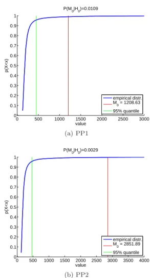
Figure 6 shows the global test results for the dif-ference measure d2
using PP1 and PP2. The global hypothesis of equal sample means is rejected and a statistically significant difference between the shape distribution of SG and CG is established (p= 0.0109 for PP1 andp= 0.0029 for PP2 withp=P(M0|H0)). The smaller p-value for PP2 seems to be due to the volume information being spread into the 24 skeletal positions instead of into a single feature. The feature-by-feature test will highlight this fact in the next sec-tion. Intermediate results of the proposed hypothesis test procedure are shown in Figure 3 on the basis of a selected GOP. Further visualizations of the procedure can be found in the Supplementary Material.
0 500 1000 1500 2000 2500 3000 0
0.1 0.2 0.3 0.4 0.5 0.6 0.7 0.8 0.9 1
value
p(X<x)
P(M
0|H0)=0.0109
empirical distr. M
0 = 1208.63 95% quantile
(a) PP1
0 500 1000 1500 2000 2500 3000 3500 4000 0
0.1 0.2 0.3 0.4 0.5 0.6 0.7 0.8 0.9 1
value
p(X<x)
P(M
0|H0)=0.0029
empirical distr. M
0 = 2851.89 95% quantile
(b) PP2
Fig. 6: Global test results using PP1 in (a) and PP2 in (b). The empirical distribution of Ml, l = 1, . . . ,30,000 is shown together withM0and the 95% quantile of the empirical distribution.
evaluation of the scaled CPNG scores matrix ZComp
(see Section 4). The CPNG scores matrix is calculated for SG and CG using both pre-processing methods. Thus, the DiProPerm test is calculated in Euclidean space using standard Euclidean statistics in contrast to the proposed hypothesis test, which is performed in the non-Euclidean s-rep space using the CPNG back-ward means. An interesting open problem is to ex-tend a method such as DiProPerm in an intrinsic way: in other words to perform DiProPerm using Manifold geodesic distances.
Table 1 summarizes all global test results. We used 30,000 permutations in all settings to be consistent with Section 6.2.2. The DiProPerm test does not re-quire such a high number of permutations in contrast to the proposed global test. Simulations, reported in the Supplementary Material, reveals that a large per-mutation size is needed to obtain stable results be-cause of the Mahalanobis distance. DiProPerm was carried out using a mean difference (MD) test statistic as recommended in [46]. The DWD-DiProPerm
per-Table 1: Empirical p-value results using difference measured2
for the proposed global hypothesis test in comparison with results obtained by DiProPerm. Two different pre-processing steps were applied: (PP1) Full Procrustes alignment with scaling. (PP2) Full Pro-crustes alignment without scaling. Three different pro-jection directions were used for DiProPerm.
method empirical p-value
PP1 PP2
Mahalanobis distance
difference measured2 0.0109 0.0029
DiProPerm using MD-statistic DWD direction vector 0.0074 0.0038
SVM direction vector 0.0119 0.0136
formance was comparable to the Mahalanobis distance results. The support vector machine (SVM) results of DiProPerm were less powerful, probably due to data pilling effects. All results are statistically significant at the level ofα= 0.05.
7.3 Single GOP test results
The global shape analysis of hippocampi in the pre-vious section can not indicate local shape differences. Interesting structural changes of the surface are often reflected by a few GOPs, e.g., the local bending of an area. Therefore, the proposed threshold correction for a feature-by-feature test in Section 6.2.7 is useful. Such a feature-by-feature test is not available from DiProPerm.
As our feature-by-feature test approach is novel for nonlinear hypotheses, there is no competing method to compare with. However, a method to evaluate the test is needed. The performance of the feature-by-feature test was evaluated using Receiver Operating Charac-teristic (ROC) curves. Selected examples of this anal-ysis are reported in Section 2.4 of the Supplementary Material. For each permutation, an ROC curve was generated from the cumulative histograms of the two permuted samples, which results in an envelope under the null distribution. In addition, an ROC curve be-tween the two true observed samples was obtained. A significant feature is indicated if the ROC curve of the observed data is close to the boundary or outside the envelope, otherwise not. A comparison of the hypoth-esis test results to this reveals the high quality of the proposed method.
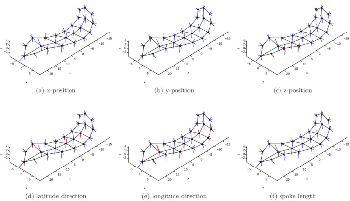
−15 −10 −5 0 5 10 15 20 −5 0 5 −2 0 2 4 x y z (a) x-position −15 −10 −5 0 5 10 15 20 −5 0 5 −2 0 2 4 x y z (b) y-position −15 −10 −5 0 5 10 15 20 −5 0 5 −2 0 2 4 x y z (c) z-position −15 −10 −5 0 5 10 15 20 −5 0 5 −2 0 2 4 x y z
(d) latitude direction
−15 −10 −5 0 5 10 15 20 −5 0 5 −2 0 2 4 x y z
(e) longitude direction
−15 −10 −5 0 5 10 15 20 −5 0 5 −2 0 2 4 x y z
(f) spoke length
Fig. 7: Significant GOPs using PP1 based on the 3×8 skeletal sheet of the SG CPNG mean. Test results are shown in (a)-(c) for the skeletal x, y and z-positions, in (d) for the latitude spoke directions, in (e) for the longitude spoke directions and in (f) for the spoke lengths. Non-significant skeletal positions are marked by small blue points and significant skeletal positions are marked by large red points. Similar, non-significant spoke directions and lengths are marked by small blue lines whereas significant spoke directions and lengths are marked by wide red lines.
y and z-positions), 66 GOPs for the latitude spoke directions (bottom, crest and top), 66 GOPs for the longitude spoke directions (bottom, crest and top), 66 GOPs for the spoke lengths (bottom, crest and top) and 1 GOP for the global scaling factor. The corrected threshold isλ= 2.2917 as defined in Section 6.2.7.
Figure 7 indicates local shape changes by highlight-ing local parts of the s-rep. Red points mark signifi-cant skeletal x, y and z-positions in the Figures (a)-(c). Non-significant skeletal positions are marked by smal-ler blue points in these figures. Five significant skeletal positions can be observed at the crest of the sheet, one in the x and y-direction and three in the z-direction. Moreover, significant spoke directions and lengths are marked by wide red lines and non-significant by thin-ner blue lines in the Figures (d)-(f). Several latitude and longitude spoke directions indicate locally signifi-cant deformations between the two groups in the Fig-ures (d)-(e). The most latitude differences that are statistically significant are on the bottom side of the skeletal sheet whereas more longitude differences are significant on the top side. Furthermore, we observe no spoke direction with simultaneously significant lat-itude and longlat-itude. This behavior should be
inves-tigated in future studies. The latitude and longitude differences could indicate local bending around the y and z-axis, respectively. Figure (f) highlights one sig-nificant spoke length on the front bottom side of the skeletal sheet.
In addition to the results presented in Figures 7, the global scaling factor τ between SG and CG was found statistically significant. The GOP |U0K| was
2.7627 where the index K corresponds to the global scale factor.
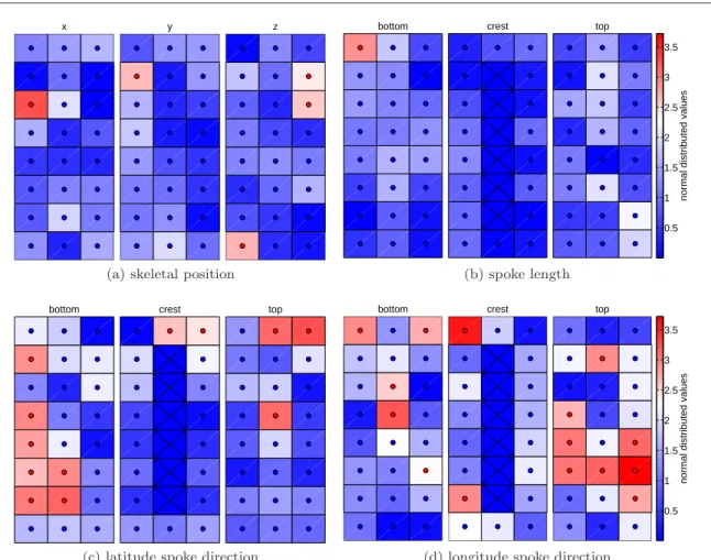
These observations and results are also emphasized by Figure 8, which shows the magnitude of signifi-cance of all GOPs except the scaling factor. In order to simplify the visualization all standard normal val-ues U0k, k = 1, . . . , K−1 are presented in absolute values. The color map is non-linear defined from blue to white to red. The corrected thresholdλdefines the color white. Blue and red visualize non-significant and significant values, respectively. The blue small circle inside a block marks whether a U0k is less than or
equal to the thresholdλ. Red small circles mark if a
U0k is greater than the threshold λand thus
Partic-x y z
(a) skeletal position
bottom crest top
normal distributed values
0.5 1 1.5 2 2.5 3 3.5
(b) spoke length
bottom crest top
(c) latitude spoke direction
bottom crest top
normal distributed values
0.5 1 1.5 2 2.5 3 3.5
(d) longitude spoke direction
Fig. 8: Colored significance map of U0k with a corrected thresholdλ= 2.2917 using PP1. Each box represents
a GOP which correspond to a skeletal atom. The color map on the left side is non-linear and has a range from blue (not significant) to white (λ) to red (significant). The circle inside each box marks whether an U0k is less
or equal than the thresholdλ(symbolized by blue) or if anU0k is greater than the thresholdλ(symbolized by
red).
ularly, several latitude and longitude spoke directions show a highly significant magnitude in Figure 8.
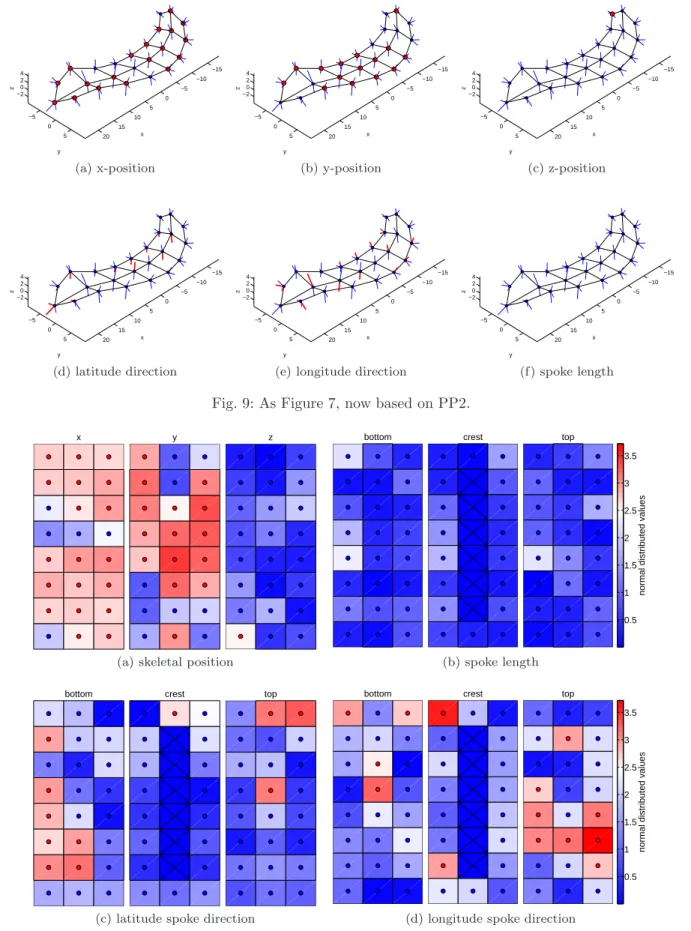
Figures 9 and 10 are identical to the two previ-ous figures except for the use of PP2 instead of PP1. Several skeletal x and y-positions are statistically sig-nificant in contrast to Figures 7 and 8 with only one significant skeletal x and y-position. The volume dif-ference between the two populations is reflected by the skeletal x and y-positions using PP2. Thus, the signif-icant skeletal x and y-positions show rather signifsignif-icant differences from a global deformation than from local deformations. However, we observe only one statisti-cally significant skeletal z-position because the skeletal sheet of the hippocampus is rather flat, as medial as possible and therefore located close to the x-y plane, wherez= 0. As a result, several skeletal z-coordinates are scaling invariant.
Nevertheless, the observation of only one signif-icant skeletal z-position in addition to no observed statistically significant spoke length in Figure 9f im-plies that we only observe statistically significant vol-ume differences in the x-y direction but not in the
z-direction. Skeletal x and y-positions equal to x = 0 and y = 0 are scaling invariant in the x and y-directions respectively. As a result, no statistically sig-nificant x-positions can be observed close tox= 0 in Figure 9a. Moreover, Figures 10c and 10d show only small differences compared to Figures 8c and 8d. Sim-ilar results between spoke directions are expected be-cause of the scaling invariance ofuij ∈S2
. The slightly different color scheme is also due to a different thresh-old.
−15 −10 −5 0 5 10 15 20 −5
0 5 −2
0 2 4
x
y
z
(a) x-position
−15 −10 −5 0 5 10 15 20 −5
0 5 −2
0 2 4
x
y
z
(b) y-position
−15 −10 −5 0 5 10 15 20 −5
0 5 −2
0 2 4
x
y
z
(c) z-position
−15 −10 −5 0 5 10 15 20 −5
0 5 −2
0 2 4
x
y
z
(d) latitude direction
−15 −10 −5 0 5 10 15 20 −5
0 5 −2
0 2 4
x
y
z
(e) longitude direction
−15 −10 −5 0 5 10 15 20 −5
0 5 −2
0 2 4
x
y
z
(f) spoke length
Fig. 9: As Figure 7, now based on PP2.
x y z
(a) skeletal position
bottom crest top
normal distributed values
0.5 1 1.5 2 2.5 3 3.5
(b) spoke length
bottom crest top
(c) latitude spoke direction
bottom crest top
normal distributed values
0.5 1 1.5 2 2.5 3 3.5
(d) longitude spoke direction
derived from 5 independent CPNG stages in Section 5 by using a pooled shape distribution, two individual shape distributions and two individual interchanged shape distributions. The second group of final fittings is described in detail in Section 3 of the Supplemen-tary Material.
8 Discussion
This paper proposes a novel method to test global and local hypotheses on Euclidean and non-Euclidean data. Important requirements of shape models are pointed out in order to test for population differences. Fur-thermore, suitable statistical methods are proposed to analyze the Euclidean and non-Euclidean elements of the models. In addition, the estimation of appropri-ate shape distributions of populations is worked out. Finally, the analysis of first episode schizophrenia pa-tients compared to controls demonstrated the power of the hypothesis test given a proper pre-processing. The effect of different pre-processings of the data are highlighted. The developed feature-by-feature test is novel and important for physicians in order to under-stand local shape changes. The method can easily be adapted for desired GOPs depending on underlying research questions. A difference measure for the anal-ysis of s-reps is proposed. The visualization of local shape changes is of great interest for the study of lo-cal rotational deformations [39] which is a subject of future studies.
The s-rep model, statistics and the fitting proce-dure resulted in accurate fittings with a high concen-tration of variance in relatively few eigenmodes. This reflects the high correspondence between the s-reps. The introduced test found significant differences be-tween the two populations. First, a statistically sig-nificant loss of hippocampal volume was observed by the global scaling factor which is in agreement with [25,28,29]. Second, a significant volume difference was observed in the x and y-directions but not in the z -direction for the aligned hippocampi. Third, several spoke directions were found as statistically significant. This study is the first study that examines direc-tional information using s-reps. The significant differ-ences of several spoke directions confirm the impor-tance of our contribution in the research of morpho-logical shape changes and encourages further research. Later studies should more deeply investigate if spoke direction differences are due to independent local de-formation of GOPs or due to local rotational defor-mation. Styner et al. [42] indicated a potential local bending of the hippocampi between the two groups. Furthermore, this study is the first study that could identify directions driving the volume change.
In general, results are challenging to compare be-tween studies of brain morphology because of different models, features and metrics. Narr et al. [29] calcu-lated a radial distance measure in addition to a mea-sure that examined the signal intensity on the basis of a surface based mesh modelling method. Also, Mamah et al. [25] used a triangulated graph representation of the hippocampi. Such models are limited compared to s-reps because the interior of an object is not de-scribed by the model itself. The model representation in McClure et al. [28] is a skeleton type which leads to less correspondence between populations and con-tains further disadvantages, e.g., all spoke length are identical on each atom. Furthermore, McClure et al. [28] applied an FDR based test approach in contrast to the FWER based approach proposed in this paper. The FDR is a less strict multiple testing criteria than the FWER. However, the discussed results are consis-tent between the studies. The s-rep model provides a relatively rich description of an object. Moreover, the proposed test procedure offers global and local linear hypothesis tests based on Euclidean and non-Euclidean GOPs. Thus, the test supports more con-sistent and sensitive interpretations of morphological changes.
This paper motivates several areas of further re-search. 1) A simplification of the s-rep fitting pro-cedure is desirable that depends on correct choice of several fitting parameters. The choice of a large num-ber of parameters might be an avoidable difficulty in the use of s-reps in clinical practice. 2) The defini-tion of an adaptive s-rep model that finds an opti-mal skeletal grid could be of relevance for the future. The grid need not to be rectangular but must corre-spond across cases of a population. 3) The hypothesis test might be extended by including image intensities in addition to morphological features. An interesting research question is the study of correlation between morphological changes and intensities. 4) An alterna-tive combining function might decrease the required large number of permutations for a global test. 5) A power study on the basis of simulated data to elab-orate further the proposed method. 6) A comparison of hippocampi between two treatment groups of first episode schizophrenia. 7) Extension of the method to hippocampi from longitudinal data. In addition, a sim-ilar hypothesis test based on the sample variance in-stead of the sample mean could be of future interest.