THE EFFECTS OF URBANIZATION ON RIPARIAN FOREST PLANT COMMUNITIES IN THE RESEARCH TRIANGLE AREA OF NORTH CAROLINA
Bianca E. Lopez
A dissertation submitted to the faculty at the University of North Carolina at Chapel Hill in partial fulfillment of the requirements for the degree of Doctor of Philosophy in the Curriculum
for the Environment and Ecology.
Chapel Hill 2017
iii ABSTRACT
Bianca E. Lopez: The effects of urbanization on riparian forest plant communities in the Research Triangle area of North Carolina
(Under the direction of Peter S. White)
Ongoing urban development is having profound impacts on ecosystems worldwide, by reducing the amount and connectivity of natural habitat and changing the local environmental conditions. Despite the ubiquity and the continued growth of urban areas, the effects of urban development on the diversity and composition of plant communities remain poorly understood. In this dissertation, I address this issue by investigating the effects of urban development on patches of remnant riparian forest in the Research Triangle area of North Carolina. To do this, I used a rural-to-urban gradient approach, comparing the plant species and environmental
and spatial variables describing habitat connectivity to explain variation in plant species
v
I dedicate this work to my parents, Kimberly Ann Moore and Alvaro Benito Lopez, who have supported me and inspired me with their continued excitement for learning about the world
around them, and to my great friend Brendan Patrick Galvin, who has seen me through.
ACKNOWLEDGMENTS
This dissertation would not have been possible without the help of many, many people. First, I would like to thank my committee members, who offered guidance, practical help, and intellectual challenges. Melissa McHale has been encouraging but also grounding, and
challenged me to place my work within the broader urban ecology field, to my benefit. Allen Hurlbert and Dean Urban provided critical statistical and theoretical advice, and Dean and Bob Peet provided logistical support for my data collection. Bob was also a reference for all questions regarding the plant communities in North Carolina, and improved my work by questioning my assumptions. Above all, Peter White was an excellent advisor, who let me work at my own pace while providing lively intellectual conversation and encouragement. My committee members have been inspiring models of scientists and academics, and if I have any regret it is that I did not make more use of their expertise.
vii
helped me in the field as well, including Dennis Tarasi, Julie Tuttle, Kyle Palmquist, Megan McClung, Peter Wilfahrt, Naomi Schwartz, Bren Galvin, and Seth Rifkin.
The Plant Ecology Lab has been a unique setting in which to pursue a graduate degree, and I have enjoyed being part of it. The students and faculty of PEL have been a crucial
sounding board, as well as a source of help with plant identification and fieldwork. Of the many individuals that have passed through PEL during my seven-year tenure, several offered particular assistance with my dissertation work. Liz Matthews was an incredibly helpful senior grad student during my first year, and continued to give me advice (and let me use her data) as my research developed. Kyle Palmquist was a mentor and a pal. Sam Tessel, Derrick Poindexter, and Alan Weakley helped me with plant ID (especially with the sedges), and Carol Ann McCormick facilitated my use of the herbarium for reference. Pat Gensel has been a role model and a source of solid advice on research and career choices. Like Pat, Michael Lee could always be counted on for great questions and suggestions on my research. Michael also made the office a fun place to be, and was equal parts helpful and mischievous. Chris Payne and Dennis Tarasi were like my little brothers, and Alissa “Toots” Brown was my partner in crime. Peter Wilfahrt started when I did, left a year before me, and spent the time in between (when not dissertating, of course) plotting schemes for pizza shacks on the beach, drawing pterodactyls on the office chalkboard, and generally making going to work that much better.
Brian Evans and Robbie Burger were excellent resources to talk urban ecology, and were always down for a trip to Linda’s. I benefited so much from talking to CEE students in other fields about ecology, and some of these talks have led me to move outside of my comfort zone in my future research. Naomi Schwartz, Tony Mayer, Diamond Ebanks, Catie Alves, Chris Hakkenberg, Sierra Woodruff, and Clare Fieseler, among others, have always been game to talk to me about my research and give me a different perspective on my work. Ultimately, my writing
companions, Sierra Woodruff, Peter Wilfahrt, Dennis Tarasi, Alissa Brown, and Alan Kinlaw, made starting and finishing this dissertation possible. I will be forever indebted to Alan for helping me format my dissertation and saving me a seat at coffee shops.
ix
TABLE OF CONTENTS
LIST OF TABLES ... xiii
LIST OF FIGURES ... xv
CHAPTER 1: Introduction ... 1
Introduction ... 1
Description of study area and research scope ... 4
Chapter summaries ... 6
References ... 8
CHAPTER 2: The four filters of urbanization and their effects on forest plant taxonomic, functional, and phylogenetic diversity ... 12
Introduction ... 12
Methods... 15
Study area and site selection ... 15
Plant community data ... 16
Trait data ... 16
Phylogeny construction ... 17
Diversity measures ... 18
Four filters of urbanization ... 20
Metamodel development ... 22
Results ... 25
Discussion ... 27
Effects of the urban environment ... 28
Habitat transformation, fragmentation, and human pressure ... 29
Implications for urban conservation ... 31
The four filters of urbanization and comparative urban ecology ... 33
References ... 44
CHAPTER 3: Using plant traits to determine the opportunities and limitations of riparian forest restoration in urban areas ... 52
Introduction ... 52
Methods... 55
Plant community data ... 55
Reference community data ... 56
Trait data ... 57
Environmental and land cover data ... 58
Data analysis: Comparison to restoration targets ... 59
Data analysis: Changes in traits with urbanization ... 63
Results ... 64
Dissimilarity between sample sites and reference community types ... 64
Differences in species composition between urban sites and restoration targets ... 65
xi
Changes in traits with urbanization ... 69
Comparison of urban sites to reference community types ... 70
Implications for restoration ... 72
References ... 85
CHAPTER 4: Plant species’ responses to habitat connectivity and urban environments depend on nativity and seed dispersal mode ... 91
Introduction ... 91
Methods... 95
Study system ... 95
Site selection ... 95
Plant community data ... 96
Environmental and landscape data ... 97
Statistical analyses: Habitat connectivity models ... 98
Statistical analyses: Redundancy analysis ... 101
Results ... 102
Connectivity model- and variable selection ... 103
Environmental and landscape variable selection ... 104
Variance partitioning ... 105
Discussion ... 106
Effects of land use on habitat connectivity and dispersal limitation ... 107
Environmental effects on species composition ... 110
Effects of urban land cover surrounding sites ... 111
Implications for conservation in urban areas ... 111
CHAPTER 5: Conclusion ... 132
Habitat area ... 132
Habitat fragmentation ... 134
Environmental effects ... 135
Species introductions ... 138
Limitations and future directions ... 140
References ... 143
APPENDIX A: Categorical trait data for species in dataset ... 146
APPENDIX B: Trait data acquisition and processing from try database ... 174
APPENDIX C: Missing and added species from urban sites compared to reference community types ... 178
APPENDIX D: Categorization of land use/land cover data for creation of resistance rasters to make least-cost paths ... 180
xiii
LIST OF TABLES
Table 2.1. Predictions of the net effects of the four filters of urbanization
on plant biodiversity... 35
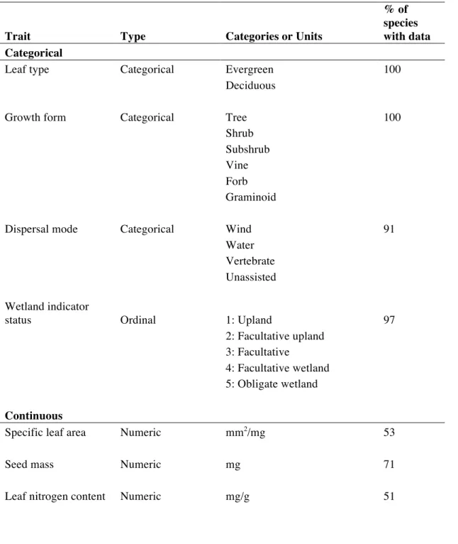
Table 2.2. Information on traits used in analyses of functional diversity... 36
Table 2.3. Model fit statistics for structural equation models...37
Table 2.4. Overview of observed effects of biodiversity “filters” on measures
of biodiversity... 38
Table 3.1. Traits used in analyses with predicted responses to urbanization
and hypothesized mechanisms... 74
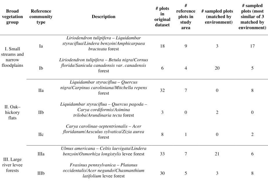
Table 3.2. Descriptions of reference community types (from Matthews et al.
2011) with number of plots matched with each... 76
Table 3.3. Results of Fisher's exact test comparing the ratio of species in each trait category between missing or added species and a larger
species group...78
Table 3.4. Results of multiple regression analyses of the prevalence of species’ traits in communities in response to urbanization
measures...79
Table 4.1. Description of variables used in redundancy analyses...114
Table 4.2. Forward-selected spatial, environmental, and landscape variables predicting species composition of species groups in redundancy
analysis...115
Table 4.3. Results of variance partitioning with tests of significance for pure fractions of variation in species composition explained by spatial,
environmental, and landscape variables... 116
Table A.1. Categorical trait data used in analyses...146
Table B.1. Matches between species in community dataset and species in TRY
Table B.2. Database sources of data on each continuous trait, accessed from
the TRY database... 179
Table C.1. Species frequently missing from and species frequently added to the 14 most urban plots in the dataset, when compared to reference
community type descriptions... 182
Table D.1. Comparison of land use/land cover categories from the National Land Cover Dataset in 1992 and 2011, with designated resistance
xv
LIST OF FIGURES
Figure 2.1. Meta-model diagram of relationships between predictor variables
(urbanization filters) and plant biodiversity... 45
Figure 2.2. Bivariate relationships between diversity measures and population
density with standard errors... 46
Figure 2.3. Bivariate relationships between diversity measures and forest cover,
with standard errors... 47
Figure 2.4. Results of structural equation models predicting taxonomic richness, native and exotic species richness, phylogenetic richness, and
phylogenetic evenness... 48
Figure 3.1. Changes in the proportions of traits of added and missing species
with increasing urbanization... 74
Figure 3.2. Changes in the proportions of categorical traits of all species with
increasing urbanization... 75
Figure 4.1. Map of impervious surface cover in the Research Triangle area (30 m-resolution data from the National Land Cover Dataset)
and sample sites... 76
Figure 4.2. Maps depicting connectivity networks, minimum spanning trees connecting sites, and graphed MEM eigenvectors for Euclidean distance, 1992 least-cost paths, 2011 least-cost paths, and
along-stream distance... 85
Figure F.1. Risk function for at least one redeemed antibiotic prescription, by age (in months) through the first year of life, stratified by
season of birth, Denmark 2004-2012... 104
Figure 4.3. Conceptual flow diagram of data analysis steps... 105
Figure 4.4. Effective distance along least-cost paths was generally higher
using 2011 land use data than using 1992 data... 108
Figure 4.5. Variation in species composition of each species group explained
by spatial variables for different connectivity models... 109
Figure 4.6. Results of variance partitioning of species composition explained
CHAPTER 1: INTRODUCTION
INTRODUCTION
Over half of the people in the world live in cities (United Nations 2015) and urban areas are continuing to grow both globally (Seto et al. 2011) and across the Southeastern United States (Terando et al. 2014). Despite the ubiquity of human settlements and well-documented effects of urban development on the environment (e.g., the urban heat island effect [Oke 1995], reductions in air and water quality [Pickett et al. 2011]), the impacts of urbanization on ecosystems remain poorly understood. This is because until the 1970’s, ecologists mainly chose to study relatively pristine ecosystems rather than pursue research in urban areas (McDonnell and Pickett 1990, McDonnell 2011). Since that time, the field of urban ecology has emerged to address this knowledge gap.
Early research in urban ecology focused on documenting changes in the abundance and diversity of organisms as well as ecological processes (e.g., nitrogen cycling, leaf litter
decomposition) with urbanization (McDonnell et al. 1997). Although some studies have used herbarium records and other historical accounts of species occurrences to identify changes in species composition in cities over time (Van der Veken et al. 2004, Stehlik et al. 2007, Hahs et al. 2009, Duncan et al. 2011), most have used a spatial urban-to-rural gradient approach,
2
sites (e.g., impervious surface cover, population density; McDonnell and Hahs 2008). These spatial gradients stand in as a space-for-time substitution for the process of urbanization, which is generally more difficult to study, as historical pre-urbanization records are somewhat scarce. These studies have collectively shown several general trends across cities. One is an increase in exotic species in many urban areas (Lososová et al. 2012, Aronson et al. 2015), which contribute to a global homogenization of species composition across cities (McKinney 2006, Groffman et al. 2014). Early on, some researchers recognized that different species respond to urbanization differently; some species act as “urban avoiders”, while others tend to be “urban tolerators” or “urban exploiters” (Blair 1996). Changes to the local environment, the amount and configuration of habitat, and the introductions of novel species can all have effects on natural communities within and around cities (Williams et al. 2009). Some ecologists have suggested that these changes create "novel ecosystems" that require their own theories and considerations for management (Seastedt et al. 2008, Kowarik 2011), while others have pointed out similarities between many of the effects seen in urban areas and examples in more “natural” settings, suggesting that existing ecological theories (e.g., Island Biogeography, metacommunity theory) can and should be applied to urban ecosystems (Niemelä 1999, Faeth et al. 2011).
One aspect of urban areas that makes them markedly different from many other ecosystems is the strength of the effects of human decisions, both at the individual and
institutional level. This has led some urban ecologists to work collaboratively with researchers from the social sciences to treat cities as socio-ecological systems. Research of this nature has been termed “ecology of cities”, in contrast with “ecology in cities”, the single-discipline
the two urban Long Term Ecological Research centers in Baltimore, MD and Phoenix, AZ. Recently, Childers et al. (2015) proposed a third emphasis for urban ecology research, “ecology for cities”, which attempts to make connections between ecological research, urban planning and design, and the needs of urban residents to create more sustainable, livable cities. While ecology in cities remains the most common type of urban ecology research being carried out today, the rise of ecology of and for cities has increased recognition of people as being an important
component of urban ecosystems (Pickett et al. 2013, Wu 2014, McDonnell and MacGregor-Fors 2016, McPhearson et al. 2016, Schwarz and Herrmann 2016).
However, there is still much to learn about ecology in cities. In particular, since the early years of urban-to-rural gradient analysis, there has been a push towards moving past the simple documenting of patterns to understanding changes in ecosystem processes such as resource availability, disturbance, species interactions, and dispersal (Shochat et al. 2006, Faeth et al. 2011). McDonnell and Hahs (2013) have called this “moving beyond the ‘low-hanging fruit’” of urban biodiversity research. They propose that in order to provide robust and useful
recommendations to conservation practitioners and urban planners, it is critical to have a general, synthetic understanding of the mechanisms underlying observed responses of natural
4
In this dissertation, I carried out three studies based on one dataset of plant communities spanning an urban-to-rural gradient to answer the broad research question: How is urban
development influencing the plant species that are found in remnant riparian forest? I
emphasized the use of informative measures of ecological drivers influenced by urbanization (e.g., habitat connectivity, environmental conditions) and plant community responses. In these three studies (Chapters 2-4), I use different analytical methods and different response variables describing measures of community structure: diversity, trait composition, and beta diversity (species turnover or changes in species composition across sites). Here, I briefly summarize each of these chapters, highlighting their contributions to understanding mechanisms underlying community changes with urbanization and to promoting comparability with other urban ecology studies.
DESCRIPTION OF STUDY AREA AND RESEARCH SCOPE
Australia. Few studies have been conducted in the southeastern U.S. (but see Price et al. 2006, Burton and Samuelson 2008, Minor and Urban 2009, Nagy and Lockaby 2011), despite ongoing urban development in this region (Brown et al. 2005, Terando et al. 2014). However, in the last several years the Research Triangle has become a hotspot for new urban ecology research, specifically regarding changes to streams and insect populations (Sudduth et al. 2011, Inkilainen et al. 2013, Somers et al. 2013, Dale and Frank 2014, Youngsteadt et al. 2015, Meineke et al. 2016).
The large amount of forest in the Research Triangle area makes it an ideal study system for assessing the effects of urbanization on forests. This forest is mostly secondary, having been cleared for agriculture or grazing, or selectively harvested for timber. Much of the forest in the Triangle is found in riparian buffers that are protected from development by ordinances. Riparian forests in the North Carolina Piedmont (which includes the Research Triangle) have high plant biodiversity, particularly in the floodplains of small streams (Matthews et al. 2011), which I focused on for my dissertation. Riparian forest also provides important ecosystem services, such as maintaining water quality and moderating flooding (Peterjohn and Correl 1984, Sweeney et al. 2004, Newham et al. 2011).
I sampled sites along an urbanization gradient defined by the amount of impervious surface cover surrounding sites within a 1 km buffer. The urbanization gradient I sampled was short, with a maximum impervious surface cover of about 25%. This partially reflects the fact that all sites were located within forest on public lands (for purposes of gaining legal access), which are mostly relatively large patches compared to small forested areas on private lands. Study sites were also limited by the size of the forest plots I used (300-500 m2
6
many other studies, the gradient actually captured here spans mainly from rural to suburban areas, as few sites are located close to the center of a city.
CHAPTER SUMMARIES
In Chapter 2, I use structural equation modeling to examine the effects of forest cover, forest fragmentation, environmental variables related to urbanization (temperature, soil
phosphorus content, and stream incision), and human population density on plant biodiversity. This analysis tests predictions made by Williams et al. (2009) for how the “four filters” of urbanization (habitat transformation, fragmentation, the urban environment, and human preferences) influence plant taxonomic, functional, and phylogenetic diversity. I describe how this analysis can be applied in multiple different urban areas, and how I expect the results to differ in different settings.
In Chapter 3, I analyze changes in the composition of species’ traits relating to
In Chapter 4, I assess the ability of environmental variables and spatial variables
representing habitat connectivity to explain variation in plant species composition across sites. I create multiple models of habitat connectivity between sites and use these to determine whether land use between sites influences species’ distributions across space. This chapter speaks to the importance of different ecological processes (environmental filtering and dispersal) for
structuring plant communities in an urban landscape.
8
REFERENCES
Aronson, M. F. J., S. N. Handel, I. P. La Puma, and S. E. Clemants. 2015. Urbanization promotes non-native woody species and diverse plant assemblages in the New York metropolitan region. Urban Ecosystems 18:31–45.
Blair, R. B. 1996. Land use and avian species diversity along an urban gradient. Ecological Applications 6:506–519.
Brown, D. G., K. M. Johnson, T. R. Loveland, and D. M. Theobald. 2005. Rural land-use trends in the conterminous United States, 1950-2000. Ecological Applications 15:1851–1863. Burton, M. L., and L. J. Samuelson. 2008. Influence of urbanization on riparian forest diversity
and structure in the Georgia Piedmont, US. Plant Ecology 195:99–115.
Childers, D. L., M. L. Cadenasso, J. M. Grove, V. Marshall, B. McGrath, and S. T. A. Pickett. 2015. An ecology for cities: A transformational nexus of design and ecology to advance climate change resilience and urban sustainability. Sustainability 7:3774–3791.
Dale, A. G., and S. D. Frank. 2014. Urban warming trumps natural enemy regulation of herbivorous pests. Ecological Applications 24:1596–1607.
Duncan, R. P., S. E. Clemants, R. T. Corlett, A. K. Hahs, M. A. McCarthy, M. J. McDonnell, M. W. Schwartz, K. Thompson, P. A. Vesk, and N. S. G. Williams. 2011. Plant traits and extinction in urban areas: a meta-analysis of 11 cities. Global Ecology and Biogeography 20:509–519.
Faeth, S. H., C. Bang, and S. Saari. 2011. Urban biodiversity: Patterns and mechanisms. Annals of the New York Academy of Sciences 1223:69–81.
Grimm, N. B., J. M. Grove, S. T. A. Pickett, and C. L. Redman. 2000. Integrated approaches to long-term studies of urban ecological systems. BioScience 50:571–584.
Groffman, P. M., J. Cavender-Bares, N. D. Bettez, J. M. Grove, S. J. Hall, J. B. Heffernan, S. E. Hobbie, K. L. Larson, J. L. Morse, C. Neill, and K. Nelson. 2014. Ecological
homogenization of urban America. Frontiers in Ecology and the Environment 12:74–81. Hahs, A. K., M. J. McDonnell, M. A. McCarthy, P. A. Vesk, R. T. Corlett, B. A. Norton, S. E.
Clemants, R. P. Duncan, K. Thompson, M. W. Schwartz, and N. S. G. Williams. 2009. A global synthesis of plant extinction rates in urban areas. Ecology Letters 12:1165–1173. Inkilainen, E. N. M., M. R. McHale, G. B. Blank, A. L. James, and E. Nikinmaa. 2013. The role
of residential urban forest in regulating throughfall: A case study in Raleigh, North Carolina, USA. Landscape and Urban Planning 119:91–103.
Lososová, Z., M. Chytrý, L. Tichý, J. Danihelka, K. Fajmon, O. Hájek, K. Kintrová, I. Kühn, D. Láníková, Z. Otýpková, and V. Řehořek. 2012. Native and alien floras in urban habitats: A comparison across 32 cities of central Europe. Global Ecology and Biogeography 21:545– 555.
Matthews, E. R., R. K. Peet, and A. S. Weakley. 2011. Classification and description of alluvial plant communities of the Piedmont region, North Carolina, USA. Applied Vegetation Science 14:485–505.
McDonnell, M. 2011. The history of urban ecology: An ecologist’s perspective. Pages 5–13 in Urban ecology: Patterns, processes and application. Oxford University Press, Oxford, United Kingdom.
McDonnell, M. J., and A. K. Hahs. 2008. The use of gradient analysis studies in advacing our understanding of the ecology of urbanizing landscapes: Current status and future directions. Landscape Ecology 23:1143–1155.
McDonnell, M. J., and A. K. Hahs. 2013. The future of urban biodiversity: Moving beyond the low hanging fruit. Urban Ecosystems 16:397–409.
McDonnell, M. J., and I. MacGregor-Fors. 2016. The ecological future of cities. Science 352:936–938.
McDonnell, M. J., and S. T. A. Pickett. 1990. Ecosystem structure and function along gradients: An unexploited urban-rural opportunity for ecology. Ecology 71:1232–1237.
McDonnell, M. J., S. T. A. Pickett, P. Groffman, P. Bohlen, R. V. Pouyat, W. C. Zipperer, R. W. Parmelee, M. M. Carreiro, and K. Medley. 1997. Ecosystem processes along an urban to rural gradient. Urban Ecosystems 1:21–36.
McKinney, M. L. 2006. Urbanization as a major cause of biotic homogenization. Biological Conservation 127:247–260.
McPhearson, T., S. T. A. Pickett, and N. B. Grimm. 2016. Advancing urban ecology toward a science of cities. BioScience 66:198–212.
Meineke, E., E. Youngsteadt, R. R. Dunn, and S. D. Frank. 2016. Urban warming reduces aboveground carbon storage. Proceedings of the Royal Society B: Biological Sciences 283. Minor, E. S., and D. Urban. 2009. Forest bird communities across a gradient of urban
development. Urban Ecosystems 13:51–71.
10 180.
Niemelä, J. 1999. Is there a need for a theory of urban ecology? Urban Ecosystems 3:57–65. Oke, T. R. 1995. The heat island of the urban boundary layer: Characteristics, causes and effects.
Pages 81–107 in Wind Climate in Cities. Springer Netherlands, Dordrecht.
Peterjohn, W. P., and D. L. Correl. 1984. Nutrient Dynamics in an Agricultural Watershed : Observations on the Role of A Riparian Forest. Ecology 65:1466–1475.
Pickett, S. T. A., C. G. Boone, B. P. McGrath, M. L. Cadenasso, D. L. Childers, L. A. Ogden, M. McHale, and J. M. Grove. 2013. Ecological science and transformation to the sustainable city. Cities 32:S10–S20.
Pickett, S. T. A., W. R. Burch Jr., S. E. Dalton, T. W. Foresman, J. M. Grove, and R. Rowntree. 1997. A conceptual framework for the study of human ecosystems in urban areas. Urban Ecosystems 1:185–199.
Pickett, S. T. A., M. L. Cadenasso, J. M. Grove, C. G. Boone, P. M. Groffman, E. Irwin, S. S. Kaushal, V. Marshall, B. P. McGrath, C. H. Nilon, R. V. Pouyat, K. Szlavecz, A. Troy, and P. Warren. 2011. Urban ecological systems: Scientific foundations and a decade of
progress. Journal of Environmental Management 92:331–362.
Price, S. J., M. E. Dorcas, A. L. Gallant, R. W. Klaver, and J. D. Willson. 2006. Three decades of urbanization: Estimating the impact of land-cover change on stream salamander
populations. Biological Conservation 133:436–441.
Schwarz, K., and D. L. Herrmann. 2016. The subtle, yet radical, shift to ecology for cities. Frontiers in Ecology and the Environment 14:296–297.
Seastedt, T. R., R. J. Hobbs, and K. N. Suding. 2008. Management of novel ecosystems: Are novel approaches required? Frontiers in Ecology and the Environment 6:547–553.
Seto, K. C., M. Fragkias, B. Güneralp, and M. K. Reilly. 2011. A meta-analysis of global urban land expansion. PloS One 6:e23777.
Shochat, E., P. S. Warren, S. H. Faeth, N. E. McIntyre, and D. Hope. 2006. From patterns to emerging process in mechanistic urban ecology. Trends in Ecology and Evolution 21:186– 191.
Somers, K. A., E. S. Bernhardt, J. B. Grace, B. A. Hassett, E. B. Sudduth, S. Wang, and D. L. Urban. 2013. Streams in the urban heat island: Spatial and temporal variability in
temperature. Freshwater Science 32:309–326.
Sudduth, E. B., B. A. Hassett, and P. Cada. 2011. Testing the field of dreams hypothesis: Functional responses to urbanization and restoration in stream ecosystems. Ecological Applications 21:1972–1988.
Sweeney, B. W., T. L. Bott, J. K. Jackson, L. A. Kaplan, J. . D. Newbold, L. J. Standley, W. C. Hession, and R. J. Horwitz. 2004. Riparian deforestation, stream narrowing, and loss of stream ecosystem services. Proceedings of the National Academy of Sciences of the United States of America 101:14132–14137.
Terando, A. J., J. Costanza, C. Belyea, R. R. Dunn, A. Mckerrow, and J. A. Collazo. 2014. The southern megalopolis: Using the past to predict the future of urban sprawl in the Southeast U.S. PloS one 9.
U.S. Census Bureau Population Division. 2016. Annual estimates of the resident population by sex, race, and Hispanic origin for the United States, states, and counties: April 1, 2010 to July 1, 2015.
United Nations. 2015. World urbanization prospects: The 2014 revision. New York. Van der Veken, S., K. Verheyen, and M. Hermy. 2004. Plant species loss in an urban area
(Turnhout, Belgium) from 1880 to 1999 and its environmental determinants. Flora 199:516–523.
Williams, N. S. G., M. W. Schwartz, P. A. Vesk, M. A. McCarthy, A. K. Hahs, S. E. Clemants, R. T. Corlett, R. P. Duncan, B. A. Norton, K. Thompson, and M. J. McDonnell. 2009. A conceptual framework for predicting the effects of urban environments on floras. Journal of Ecology 97:4–9.
Wu, J. 2014. Urban ecology and sustainability: The state of the science and future directions. Landscape and Urban Planning 125:209–221.
Youngsteadt, E., A. G. Dale, A. J. Terando, R. R. Dunn, and S. D. Frank. 2015. Do cities
12
CHAPTER 2: THE FOUR FILTERS OF URBANIZATION AND THEIR EFFECTS ON FOREST PLANT TAXONOMIC, FUNCTIONAL, AND PHYLOGENETIC DIVERSITY
INTRODUCTION
Conserving biodiversity in urban areas is important for maintaining functioning ecosystems and the services they provide, such as clean air and water, aesthetic value, and connections to nature, to the billions of people that live in cities (Dearborn and Kark 2010). However, urban development can also have major impacts on biodiversity, often limiting the suite of native species that persist in urban environments while encouraging the establishment of introduced and anthropophilic species such as ornamental plants and pigeons (Blair 1996, Zerbe et al. 2003). Over the last several decades, many studies have documented changes in species richness along urban-to-rural spatial gradients (reviewed by McKinney 2008, McDonnell and Hahs 2008). A few studies have also examined the effects of urbanization on functional or phylogenetic diversity, measures that describe the distribution of functional traits or the phylogenetic relationships between co-occurring species (Knapp et al. 2008, 2012, Nock et al. 2013, Swan et al. 2016). While this body of work has acted as an important step in the growth of the urban ecology field, its contributions to the development of tangible predictions for the effects of urbanization on biodiversity remain limited. For instance, a number of different
Difficulty in predicting the effects of urbanization on biodiversity arises from the variety of changes to ecosystems caused by urban development. Urbanization creates a spatially
heterogeneous landscape of land cover patches and alters local climate, hydrology, and
biogeochemical cycles (reviewed by Grimm et al. 2008). In recent years, research focused on the response of biodiversity to one or more of these specific drivers has increased our understanding of urban ecosystems. For example, studies have explored the effects of fine-scale land cover (Godefroid and Koedam 2007), habitat fragmentation (Angold et al. 2006, Burton and
Samuelson 2008), and trampling of vegetation (Hamberg et al. 2008) on plant species richness in urban areas. Some have gone a step further, investigating the relative importance of multiple effects of urbanization on biodiversity. Many of these studies assess the relative importance of multiple environmental changes associated with urbanization, such as warmer temperatures, added soil nutrients, and higher heavy metal concentrations, on plant species richness (e.g., Godefroid et al. 2007, Albrecht and Haider 2013, Huang et al. 2013, Schmidt et al. 2014). These studies help to identify which effects of urbanization are most important for determining plant species richness and thus should be targeted in attempts to mitigate those effects. However, few studies have assessed multiple types of drivers, such as socioeconomic factors and environmental conditions (Hope et al. 2003) or habitat fragmentation and disturbance (Hamberg et al. 2008, Ramalho et al. 2014).
14
species from establishing in urban areas (i.e., acts as a biodiversity filter) while encouraging colonization by other species (Williams et al. 2009). Habitat transformation reduces total remnant area, decreasing the total number of species that can inhabit remaining natural areas by causing the loss of habitat specialists, but can benefit species that thrive in edge habitat (Fahrig 2003, Godefroid and Koedam 2003). Fragmentation may inhibit species with limited dispersal ability from persisting in urban areas, but can also facilitate the spread of exotic species that are introduced in the matrix between remnant fragments (Fahrig 2003, von Der Lippe and Kowarik 2007, Vilà and Ibáñez 2011, Concepción et al. 2015). The urban environment filters species that cannot tolerate the novel environmental conditions, but also benefits species adapted to warmer temperatures, high nutrient availability, and other conditions created by urban development (Williams et al. 2015). Finally, human preferences are responsible for the removal of undesirable species from urban areas, but also the introduction of many new species such as ornamental plants sold in the horticultural industry (Reichard and White 2001). In addition to describing the positive and negative effects of these filters on plant diversity, Williams and colleagues (2009) make predictions for the net effect of each filter on taxonomic, functional, and phylogenetic diversity (Table 2.1). For example, they predict that urban environments have a net negative effect on taxonomic, functional, and phylogenetic diversity by creating novel environmental conditions where only a subset of the regional species pool with traits suited to those conditions are able to establish (as observed for phylogenetic diversity by Knapp et al. 2008).
This framework creates a conceptual model with which to evaluate the multiple effects of urbanization on plants, allowing for potential comparisons across studies and a more synthetic understanding of urban ecosystems. However, while many studies have referenced this
one study. Further, no study has specifically used this conceptual model to test the relative ability of the four filters of urbanization to predict plant biodiversity in urban areas. In this chapter, I use data on plant species taxonomic, functional, and phylogenetic diversity and predictor variables representing each of the four urbanization filters described by Williams et al. (2009) to test their predicted relationships between urbanization filters and diversity (Table 2.1) and evaluate the relative predictive ability of each filter. I use structural equation modeling, which allows me to assess a holistic model of the urban ecosystem, including relationships between the urbanization filters, and observe direct and indirect effects of each filter on biodiversity.
METHODS
Study area and site selection
The study was conducted in the Research Triangle area (RTA) of North Carolina, including the cities of Durham, Raleigh, Chapel Hill, and Cary. The RTA is estimated to be home to over 1.8 million people and is a rapidly growing metropolitan region (U.S. Census Bureau Population Division 2016). Urban development has been increasing in the RTA for the past several decades, particularly around the southern and central portions of the region (Cary and the Research Triangle Park), but the landscape remains highly forested (nearly 50% of land cover based on the National Land Cover Dataset [NLCD]; Homer et al. 2015). Most of the forest in this region has been exposed to prolonged human disturbance, particularly since European settlement, and much was cleared for agriculture or selectively harvested for timber.
16
fourth-order streams). Sites were selected to span a gradient of urbanization, defined as mean impervious surface cover (%) within a 1 km buffer (calculated from 30 m-resolution land cover data from the NLCD in 2006; Fry et al. 2011). The 42-500 m2
plots used in this study covered the entire sampled urbanization gradient (0-26% impervious surface cover within 1 km).
Plant community data
Plant species data were collected in the summers (May-September) of 2012-2014. At each site, I sampled vegetation within one randomly placed, rectangular plot. Plots were 10 m wide and 50 m long. Plots were placed roughly parallel to the stream and as close to the stream as possible. Within each plot, I identified and estimated the cover (a proxy for abundance) of all vascular plant species within three strata: the herbaceous layer (0-1m in height), shrub layer (1-4 m in height), and tree layer (4+ m in height). Species cover sampling followed the protocol laid out by the Carolina Vegetation Survey (Peet et al. 1998), with cover estimated to classes on a roughly logarithmic scale (0-1%, 1-2%, 2-5%, 5-10%, 10-25%, 25-50%, 50-75%, 75-95%, or 95-100%). Plants were identified to the species level when possible, but some taxa were only identified to genus or were lumped with another species when the two were difficult to
distinguish (e.g. Symphiotrichum sp., Vitis [cinerea + vulpina]).Identification was based on the Flora of Virginia (Weakley et al. 2012).
For this study, I considered only species' cover estimates from the herbaceous layer, which I expected would show more significant effects of urbanization than the larger, often longer-lived overstory. This data includes low-growing vines and shrubs as well as tree seedlings but no adult trees, tall shrubs, or canopy lianas.
Trait data
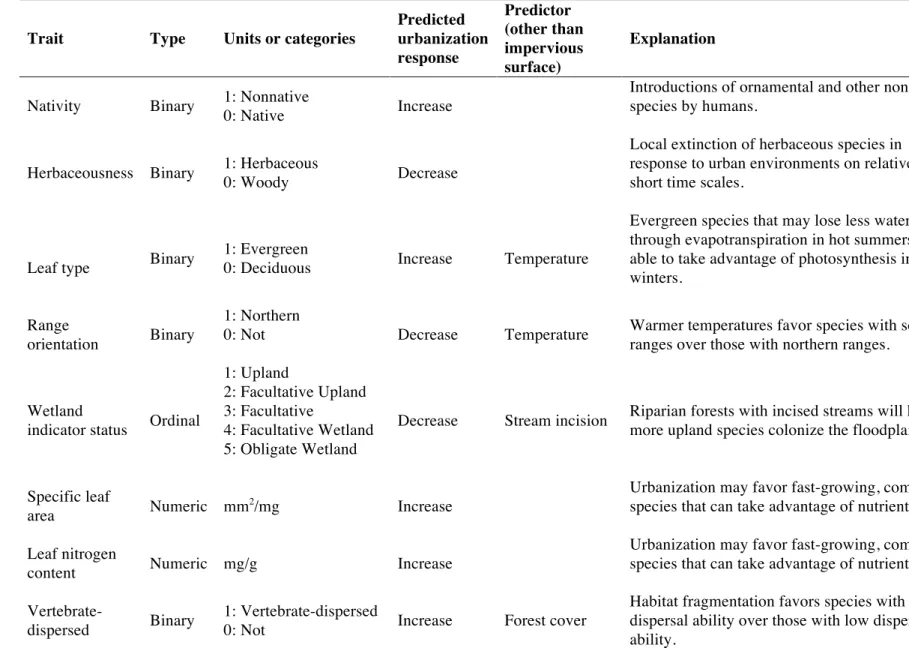
dispersal mode, wetland indicator status, specific leaf area, seed mass, and leaf nitrogen content (Table 2.2). I chose these traits because they are related to variation in dispersal ability (dispersal mode and seed mass); growth strategy, competitiveness, and stress tolerance (growth form, specific leaf area, and leaf nitrogen content); and habitat type (wetland indicator status).
Critically, these traits were also selected because I was able to find data for many of the several hundred species in the community dataset (Table 2.2). Leaf type and growth form categorization came from Weakley (2010), and wetland indicator status data came from the U.S. Army Corps of Engineers’s Wetland Plant List (Lichvar et al. 2014). Dispersal mode classification was based on a variety of published sources (but mainly from Matthews 2011 and sources within; Appendix A). Species were allowed to be categorized with more than one dispersal mode. Trait data for categorical traits can be found in Appendix A.
Continuous trait data came from the TRY database (Kattge et al. 2011), which compiles data on plant traits from many data collection efforts. For details on data selection and processing from TRY, see Appendix B. I supplemented data on seed mass and leaf nitrogen for some
species missing from TRY with a dataset compiled by Coyle et al. (2014) for Eastern North American tree species. I also found data from other sources for three of several species missing from the TRY database that had high cover within plots (maximum relative cover >10%; Appendix B). I calculated mean trait values for each species and each trait across all
observations. Seed mass, which ranged over several orders of magnitude, was log-transformed prior to calculation of functional diversity measures.
18
2016) in R (R Core Development Team 2015) to construct the phylogeny for the species in the dataset, after matching species names using the Plant List (http://www.theplantlist.org/). The S. Phylomaker function provides three options for adding missing species to the phylogeny; I used Scenario 3, which adds taxa as polytomies within parental taxa and estimates branch lengths using BLADJ (Webb and Donoghue 2005, Webb et al. 2008). This scenario is appropriate to use when calculating phylogenetic diversity to compare trends across environmental gradients (Qian and Jin 2016). After matching species names, there were several species from the community dataset still missing from the phylogeny. For those that were considered to be synonymous in the Plant List (e.g., Acer floridanum and Acer leucoderme, which are both considered subspecies of Acer saccharum) or were closely related and somewhat difficult to distinguish in the field (e.g., Carex typhina, C. aureolensis, and C. squarrosa) I lumped these combinations of species together into a single branch tip, and combined them into one species in the community data as well.
Diversity measures
Urbanization may influence plant communities by changing which species are present or absent from sites, but also by changing the relative abundance of species that are present at both rural and urban sites (Nock et al. 2013). To capture these effects, I analyzed changes in both richness measures and evenness measures, those that include information on species' relative abundances and thus capture species dominance or rarity in addition to richness. For taxonomic diversity, I calculated species richness and the Gini-Simpson index or the probability of
interspecific encounter (Hurlbert 1971), a measure of evenness that gives the probability that two randomly selected individuals in a community belong to different species.
Gaston 2006, Tucker et al. 2016). I chose to include a richness and an evenness measure for each and to use measures that I could compare easily to one another. I calculated the sum of all
pairwise functional trait differences between species (Functional Attribute Diversity [FAD]; Walker et al. 1999) as a measure of functional richness and the sum of all pairwise distances between species along a phylogenetic tree for phylogenetic richness. Functional differences between species were calculated as Gower's distances. Phylogenetic distances were calculated as phylogenetic branch lengths to the most recent common ancestor or each species pair. To
measure functional and phylogenetic evenness, I used Rao’s Quadratic Entropy, or the expected difference between any two individuals in a community, calculated as:
𝑑!" !
!!!
𝑝!𝑝!
!
!!!
where 𝑝! is the relative abundance of species 𝑖 in the community, and 𝑑!" is the difference
(functional or phylogenetic distance) between species 𝑖 and 𝑗 (Rao 1982, Botta-Dukát 2005). For
taxonomic diversity, 𝑑!" is equal to 0 when species are the same and 1 when species are different
(i.e., all species are considered to be completely and equally distinct from one another), making it equivalent to the Gini-Simpson index (Botta-Dukát 2005). Prior to calculating functional and phylogenetic diversity measures, I scaled all functional and phylogenetic distances by the maximum distance so that all pairwise distances ranged between 0 and 1 (Botta-Dukát 2005, de Bello et al. 2010). I also calculated functional diversity for each trait separately, in order to assess which traits were driving observed trends in functional diversity.
20
are effective numbers of equally abundant, equally distinct species. Hill’s numbers have the advantages of being more easily interpretable than abstract measures like Rao’s Q and obey a replication principle, meaning that they scale linearly with the pooling of unique, equally
abundant assemblages (Jost 2006, Chao et al. 2014). I calculated Hill’s numbers using equations provided by Chao et al. (2014) and de Bello et al. (2010).
Four filters of urbanization
I collected environmental data in the field to measure aspects of the urban environment and used publicly available remotely sensed and census data as proxies for habitat
transformation, fragmentation, and human preferences. To quantify habitat transformation and fragmentation, I used land cover data from the NLCD from 2011 (Homer et al. 2015) to calculate the amount and configuration of forest surrounding sample sites. As a measure of habitat
transformation, I calculated the area of forest cover present within a 1 km buffer around each site. This measure represents the amount of habitat remaining after land transformation has taken place. While it ignores past habitat area and land use legacies, which can be important for current plant diversity and species composition (Zerbe et al. 2003, Helm et al. 2006, Ramalho et al. 2014), remaining forest cover is likely an important predictor of current plant diversity based on habitat area. I calculated this measure by reclassifying 30 m-resolution land cover data into forest versus non-forest. To measure fragmentation, I defined clusters of raster cells classified as forest into patches and calculated the Landscape Division Index (LDI) of these patches. LDI is
site, first dividing the area of each forest patch by the total forest area within the buffer. I considered two variables as proxies of human preferences. These were human population density (hereafter “population density”) and median household income (hereafter “income”), both measured at the block group scale from the American Community Survey 2015 5-year estimates (Social Explorer 2017). I expected that the major effect of human preferences would be the introduction of ornamental species to the landscape, and that this effect would be higher in areas with both more people and higher income (Hope et al. 2003, Spear et al. 2013, Concepción et al. 2016). I expected that income alone would be a weaker predictor of plant diversity than population density. However, population density is a crude measure of overall human impacts (Thompson and Jones 1999), including inputs of nutrients via fertilizer
application, trampling of vegetation, and creation of pollutants and warmer temperatures from vehicles and other forms of combustion, among other effects.
I measured three components of urban development, related to the urban heat island effect (UHI), the urban stream syndrome (USS), and additions of soil nutrients to urban areas. The UHI is the phenomenon of cities being warmer than surrounding rural areas, and is a
function of waste heat from human activities such as driving and absorption of radiation by built surfaces that is released at night (Oke 1995). As a measure of the UHI, I measured air
22
bring large volumes of water into streams along with fertilizer, pollutants, and other materials (Walsh et al. 2005b). One facet of the USS is stream incision, or stream channel deepening, which occurs as a result of rapid water flow in streams during and following storms, and can lead to lowered water tables and changes in flood regimes (Groffman et al. 2003). I quantified stream incision by estimating the width and depth of the stream at each sample site and calculated a depth:width ratio. Finally, I collected soil samples at each site and measured available
phosphorus content as an indicator of nutrient addition from fertilizer runoff (Pouyat et al. 2010). Soil chemical analyses were performed by Brookside Labs, Ohio, USA.
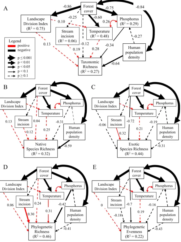
Metamodel development
I constructed a meta-model based on the predictions of Williams et al. (2009) for the effects of the four urbanization filters on biodiversity (Figure 2.1A). Because the four filters of urbanization act simultaneously to influence biodiversity and are not independent of one another, I included relationships between them in the model. Specifically, I hypothesized that habitat transformation contributes to fragmentation (Stenhouse 2004), and both habitat conversion and fragmentation promote changes to environmental conditions such as warmer temperatures (Coseo and Larsen 2014; Figure 2.1A). I then made some modifications to this model to accommodate the specific data that I used to represent each filter, which I will describe below (Figure 2.1).
filters to plant biodiversity (e.g., pollutants such as heavy metals and ozone), while others may encourage plant growth and actually increase the number of species that can inhabit urban environments. Of the three aspects of the urban environment that I measured, I expected that phosphorus would have a negative effect on biodiversity but temperature and stream incision would have positive effects on biodiversity. Additions of phosphorus and other nutrients result in decreases in species richness in some systems by favoring weedy or invasive species that
24
The model I tested with data was slightly different from this modified meta-model because of the proxy variables I used to represent habitat transformation, fragmentation, and human preferences. Since I used forest cover as a measure of habitat transformation, I expected that sites with higher forest cover (and thus presumably lower habitat transformation) would experience lower levels of fragmentation, temperature, phosphorus content, and stream incision (Figure 2.1C). As measures of human preferences, I expected that income and population density would both have positive effects on biodiversity; however, the effect of population density on biodiversity is less certain, since it represents not only species introductions but also other effects of people that may reduce biodiversity. I also expected that population density may have a positive effect on phosphorus via fertilizer inputs by people (Figure 2.1C).
Statistical analyses
I used the lavaan package in R (Rosseel 2012) to fit separate structural equation models (SEMs) for each diversity measure, using the structure shown in Figure 2.1C. Before fitting the models, I examined variable distributions and bivariate relationships between all variables. Population density was log-transformed prior to analysis to reduce skewness. The results of bivariate regressions caused us to make two changes to the model structure: I removed income as a variable from the analyses since it was unrelated to any other variables, and I added an estimate of the correlation between temperature and phosphorus. Prior to model construction, I scaled the range of some predictor variables by multiplying them by factors of 10 to reduce the difference in variances. (For example, forest cover, LDI, and stream incision all ranged from 0 to 1 and were multiplied by 100 prior to SEM analysis.).
errors and p-values (Grace 2006). Census data used in this study were collected within the block group and some plots were found in the same block group unit; therefore I also used the
lavaan.survey package (Oberski 2014) to adjust the standard errors and p-values of each model for the structure of census block groups using the Satorra-Bentler correction. I report the p-values from the lavaan.survey results in the few cases when bootstrapping led to the
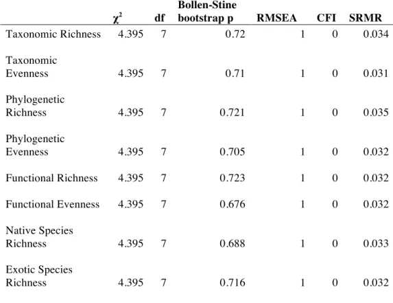
interpretation of a significant path but p-values provided by the Satorra-Bentler Robust method led to a different interpretation. I used the chi-square, RMSEA, CFI, and SRMR tests to evaluate the fit of models, as recommended by Kline (2012). I was interested in evaluating the
hypothesized model rather than comparing the fits of different models. Therefore I left non-significant paths in the models (Grace 2006). I assessed the signs of non-significant paths (p < 0.05) to test hypothesized relationships between variables. I also report marginally significant paths (p < 0.1).
In order to help interpret the results of each SEM, I performed some additional analyses on subsets of the data, including analyzing data on species richness of native and exotic plant species separately. I also used linear regression to analyze changes in the diversity of individual traits to help interpret patterns of functional diversity.
RESULTS
26
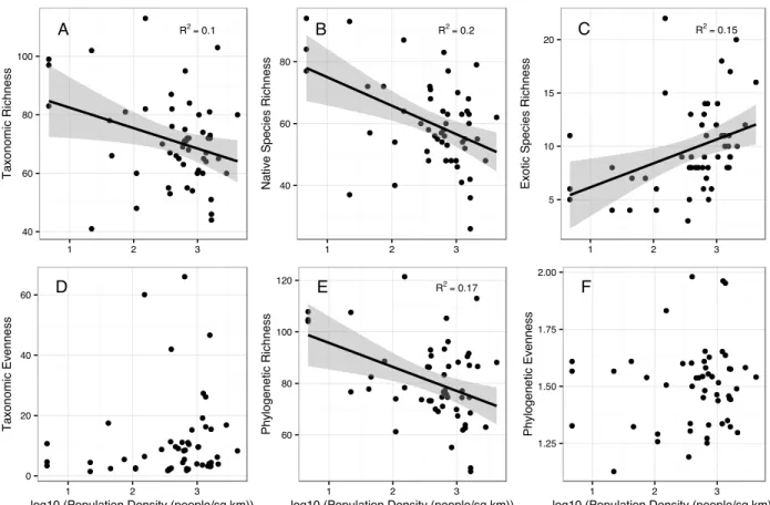
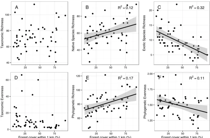
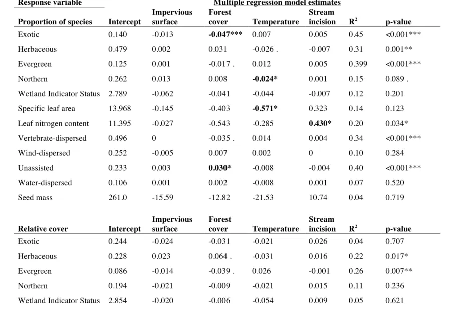
Bivariate relationships between variables showed that there were strong relationships between forest cover and LDI (r = -0.86), temperature (r = -0.69), population density (r = -0.84), and phosphorus (r = -0.51). Temperature was also correlated with LDI (r = 0.61), population density (r = 0.49), and phosphorus (r = 0.53). There was significant correlation between diversity measures, particularly between taxonomic and phylogenetic richness (r = 0.83). Taxonomic richness had a negative relationship with population density, as did native species richness and phylogenetic richness (Figure 2). Native species richness increased and exotic species richness decreased with increasing forest cover, while taxonomic richness overall showed no change with forest cover (Figure 3). In addition, phylogenetic richness increased and phylogenetic evenness decreased with increasing forest cover (Figure 3). Phylogenetic richness was also negatively correlated with LDI (r = -0.37) and phosphorus (r = -0.42), while phylogenetic evenness was positively correlated with LDI (r = 0.32) and temperature (r = 0.33). Functional evenness was positively correlated with stream incision (r = 0.45). Neither taxonomic evenness nor functional richness showed significant relationships with any predictors.
All SEMs fit the data (Table 2.3) and explained between 14 and 46% of the variation in diversity measures (Figure 2.4). Most of the variation in LDI was explained by forest cover (R2
= 0.75; Figure 2.4A). The model also explained much of the variation in temperature (R2
= 0.48), which was significantly related to forest cover (p = 0.008) but not LDI (p = 0.660). Phosphorus content was significantly explained by forest cover (R2
= 0.29, p=0.001) but not population density (p = 0.215), and was correlated with temperature (p = 0.078). Stream incision was not explained by the other predictors in the model.
decreased with increasing population density (R2
= 0.27, p = 0.033; Figure 2.4A), which was also true for native species richness (R2
= 0.32, p = 0.021; Figure 2.4B). Exotic species richness decreased with increasing forest cover (R2
= 0.44; p = 0.051; Figure 2.4C) and increased with increasing stream incision (p = 0.096). Species evenness was not explained by any predictor variables.
Phylogenetic richness was predicted by the three environmental variables (R2
= 0.46; Figure 4D), with lower phylogenetic richness in sites with high phosphorus content (p = 0.017) but higher phylogenetic richness in sites with warmer temperatures (p = 0.086) and more incised streams (p = 0.048). In contrast, phylogenetic evenness decreased with increasing forest cover (R2
= 0.22, p = 0.054; Figure 2.4E).
Functional richness was not significantly related to any predictors in the SEM, but functional evenness increased with increasing stream incision (R2
= 0.22, p = 0.004). This trend was explained to some extent by a positive relationship between functional evenness of species' leaf nitrogen content and stream incision (R2
= 0.25, p<0.001). Data for continuous functional traits such as leaf nitrogen content were not available for many species in the dataset, accounting for less than 50% of the cover for 8 of the 42 plots. However, when I removed these plots from functional diversity analyses, I saw no significant changes in the results.
DISCUSSION
28
limiting the diversity of plant communities, while others increased diversity. In addition, some predictors such as forest cover had both indirect and direct effects on biodiversity.
Effects of the urban environment
I included multiple measures of the urban environment in this study because I expected that many of them would be important predictors of biodiversity but that not all would act as biodiversity filters. Indeed, I found both negative and positive effects of the urban environment on diversity.
Phosphorus content appears to act as a biodiversity filter in my study system, supporting Williams and colleagues’ (2009) prediction that urban environments would lead to lower plant diversity. I found that sites with high phosphorus content had lower taxonomic and phylogenetic richness. I expected that this trend would result from a loss of native plant species with
Unlike phosphorus, temperature and incision had positive effects on some measures of diversity in SEMs. Warmer sites had relatively high phylogenetic richness (a marginally significant relationship), suggesting that warmer temperatures may allow phylogenetically distinct species to move into urban forest patches. These may be species with southern ranges or phylogenetically conserved traits that allow them to take advantage of the warmer temperatures, such as evergreen leaves. Stream incision had a positive relationship with functional evenness, which appeared to be driven primarily by an increase in functional evenness for leaf nitrogen. This suggests that forests adjacent to incised streams may have a higher diversity of growth strategies, on the spectrum from fast growth and high resource use to slow growth and low resource use (Wright et al. 2004). This may be due in part to changes in the flooding regime associated with stream incision and the USS. Flooding acts as a strong environmental filter in floodplains, and changes to the flooding regime could allow plants with different growth
strategies (i.e., upland and flood-intolerant species, including some exotic species) to establish in floodplains (Groffman et al. 2003, Sung et al. 2011, Catford and Jansson 2014, Brice et al. 2016). However, I did not see a corresponding change in the diversity of species' wetland
indicator statuses with stream incision. Another potential mechanism for the change in functional diversity of leaf nitrogen content is that stream incision may be correlated with other symptoms of the USS, such as nitrogen additions from stormwater runoff.
Habitat transformation, fragmentation, and human pressure
30
phylogenetic diversity are due to an increase in exotic, upland species in small forest patches. Although many exotic species in the study system come from the same families or even genera as native species, some are members of plant families unrepresented in the local native species pool that could increase phylogenetic diversity at these sites (e.g., Berberidaceae, Araliaceae, Elaeagnaceae). In addition to these direct effects, increasing forest cover had indirect positive effects on native species richness and phylogenetic richness via a decrease in phosphorus and increase in temperature.
I did not find any effects of fragmentation on diversity, but this may be due to the strong relationship between fragmentation and forest cover in the dataset. Indeed, some of the effects of fragmentation on dispersal may be accounted for in this study by differences in habitat area across sites. I found an increase in exotic species richness in sites with low forest cover, suggesting that exotics are better able to disperse into these sites or are facilitated by edge effects. Alternately, there may be effects of fragmentation on diversity that are not captured by the measure I used because it did not take any characteristics of the matrix between forest patches into account. Finally, it is also possible that fragmentation is truly not very important for diversity in the study landscape, where remnant forest is highly connected compared to some larger metropolitan areas. High connectivity between forest sites may make fragmentation effects less pronounced than they would be in landscapes with higher land cover heterogeneity.
urbanization that may influence plants, including forest cover. Although population density was not a great measure of human preferences, it did have a significant negative effect on multiple measures of diversity, apparently by reducing the number of phylogenetically distinct native species from areas of high human impact. Unfortunately, the mechanisms for this loss are not clear, and may be due to unmeasured effects such as trampling, changes in herbivore densities, or environmental effects such as pollutant additions.
Implications for urban conservation
I found both positive and negative effects of urbanization on taxonomic, functional, and phylogenetic diversity. However, it is important to note that positive effects were often
attributable to increases in exotic species, a response that may not be desirable for purposes of conserving biodiversity in urban areas and may create novel communities (Hobbs et al. 2006, Kowarik 2011). In addition, decreases in taxonomic and phylogenetic diversity in response to increased human impact and altered urban environments are concerning. These effects may mean that urban forests will be less able than rural forests to respond to changing environmental
conditions in the future (Knapp et al. 2008). Considering measures of diversity other than species richness and looking at patterns for both native and exotic species help to illuminate these
different effects.
32
effects on herbivore density and environmental conditions (Ramalho et al. 2014). However, conservation of large areas is not often feasible, particular in urban areas where land prices are high. Thus it is also important to consider ways to manage smaller habitat patches to improve their ability to harbor biodiversity.
I also found that environmental conditions associated with urbanization can have
significant impacts on biodiversity. Therefore attempting to mitigate some of the environmental impacts of urbanization could be another important strategy for conservation, particularly in small forest patches. Of the environmental variables I considered in this study, soil phosphorus availability is the clearest target for mitigation because of its negative effects on taxonomic and phylogenetic richness. Stream incision may also be a good target for mitigation since it is
associated with increased exotic species richness. Both stream incision and nutrient additions are related to the USS, resulting from stormwater runoff (Walsh et al. 2005b). Local stream
restoration, a common practice in urban areas, can reduce stream incision, but restoring flooding regimes and reducing nutrient inputs may require watershed-scale efforts (Walsh et al. 2005a, Bernhardt and Palmer 2007). Plans to maintain riparian buffers and increase green infrastructure may help to reduce the impacts of the USS.
environmental change (Cadotte et al. 2012, Srivastava et al. 2012). Thus the question of how much emphasis should be placed on exotic species management remains open. If exotic species in urban forests is a concern, education about the potential negative effects of exotic species may be a useful strategy for changing the effects of human preferences on plant communities. Future work to identify the contribution of people’s choices of what plants to keep in their yards could provide further insight into opportunities to mitigate the effects of urbanization on biodiversity.
The four filters of urbanization and comparative urban ecology
The utility of the conceptual framework developed by Williams ans colleagues (2009) is that it can apply to many urban ecosystems and allow for comparison between them. In this paper, I used this framework to develop a meta-model that can be tested in multiple cities to gain a more synthetic understanding of the effects of urbanization on biodiversity. I expect that other cities will show different trends that will improve our understanding of contingencies on the effects of urbanization on ecosystems. My system is somewhat unique in that it has lots of remnant forest and high baseline plant biodiversity. I would expect that the effects of
fragmentation are higher in cities with less connected remnant vegetation and that the effects of individual environmental factors and environmental filtering as a whole will be different in cities with different background environments, such as in different climates. Human preferences are likely more important in actively managed sites and in studies where the focus is an entire urban flora or non-remnant habitat patches.
34
maximizes the applicability of my methodology to other study systems, at least in places like the United States where remotely sensed data products and census data have comprehensive
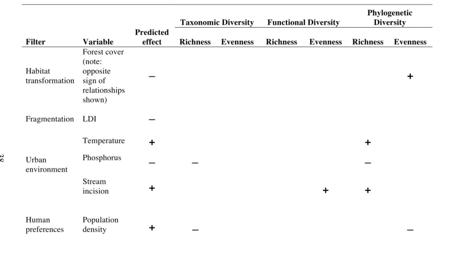
Table 2.1. Predictions of the net effects of the four filters of urbanization on plant biodiversity (modified from Williams et al. 2009).
Predicted effects on diversity
Filter Taxonomic Functional Phylogenetic Explanation
Habitat
transformation decrease decrease
Loss of specialist species from the most frequently converted habitats (e.g. wetlands). Loss of sink species.
Fragmentation decrease decrease decrease
Loss of species with limited dispersal or reproductive output and species with specialist mutualists. Gain of exotic species.
Urban
environment decrease decrease decrease
Loss of species that cannot tolerate novel environmental conditions.
Human
preferences increase increase
36
Table 2.2. Information on traits used in analyses of functional diversity.
Trait Type Categories or Units
% of species with data Categorical
Leaf type Categorical Evergreen 100
Deciduous
Growth form Categorical Tree 100
Shrub Subshrub Vine Forb Graminoid
Dispersal mode Categorical Wind 91
Water Vertebrate Unassisted
Wetland indicator
status Ordinal 1: Upland 97
2: Facultative upland 3: Facultative
4: Facultative wetland 5: Obligate wetland
Continuous
Specific leaf area Numeric mm2/mg 53
Seed mass Numeric mg 71
Table 2.3. Model fit statistics for structural equation models.
χ2 df
Bollen-Stine
bootstrap p RMSEA CFI SRMR
Taxonomic Richness 4.395 7 0.72 1 0 0.034
Taxonomic
Evenness 4.395 7 0.71 1 0 0.031
Phylogenetic
Richness 4.395 7 0.721 1 0 0.035
Phylogenetic
Evenness 4.395 7 0.705 1 0 0.032
Functional Richness 4.395 7 0.723 1 0 0.032
Functional Evenness 4.395 7 0.676 1 0 0.032
Native Species
Richness 4.395 7 0.688 1 0 0.033
Exotic Species
Table 2.4. Overview of observed effects of biodiversity “filters” on measures of biodiversity.
Taxonomic Diversity Functional Diversity
Phylogenetic Diversity
Filter Variable
Predicted
effect Richness Evenness Richness Evenness Richness Evenness
Habitat transformation
Forest cover (note: opposite sign of relationships shown)
—
+
Fragmentation LDI —
Urban environment
Temperature
+
+
Phosphorus
— — —
Stream
incision
+
+
+
Human preferences
Population
density
+
— —Figure 2.1. Meta-model diagram of relationships between predictor variables (urbanization filters) and plant biodiversity. Conceptual variables are outlined in dashed boxes and measured variables are outlined in solid boxes. Black arrows represent negative hypothesized relationships and red arrows represent positive hypothesized relationships. I hypothesized that habitat
40
Habitat transformation
Urban environment
Plant biodiversity
Habitat transformation
Fragmentation
Human preferences
Plant biodiversity
Stream incision
Temperature
Phosphorus
Human preferences Fragmentation
Forest cover Landscape
Division Index
Human population
density
Plant biodiversity
Stream incision
Temperature
Phosphorus
A
B
C
Figure 2.2. Bivariate relationships between diversity measures and population density with standard errors. Relationships with population density depend on whether analyzing data on richness for all species (A), native species (B), or exotic species (C) and whether using
presence/absence (A, E) or abundance (D, F) data. Phylogenetic richness shows a similar pattern with population density to that shown by taxonomic richness, but the relationship is slightly stronger. Linear relationships and R2
are shown only when relationship was significant (p < 0.05).
A R2=0.1
40 60 80 100
1 2 3
T axonomic Richness D 0 20 40 60
1 2 3
log10 (Population Density (people/sq km))
T
axonomic
E
venness
B R2=0.2
40 60 80
1 2 3
Nat
ive
S
pecies
Richness
E R2=0.17
60 80 100 120
1 2 3
log10 (Population Density (people/sq km))
P
hylogenet
ic
Richness
C R2=0.15
5 10 15 20
1 2 3
E xot ic S pecies Richness F 1.25 1.50 1.75 2.00
1 2 3
log10 (Population Density (people/sq km))
P
hylogenet
ic
E