FINANCIAL LOSSES FROM GENERATION OVERSUPPLY IN HYDROPOWER-DOMINANTED SYSTEMS WITH GROWING WIND CAPACITY
Yufei Su
A thesis submitted to the faculty of the University of North Carolina at Chapel Hill in partial fulfillment of the requirements of the degree of Master of Science in the Department of Environmental Sciences and Engineering in the Gillings School of Global Public Health.
Chapel Hill 2016
Approved by:
Gregory W. Characklis
J. Jason West
ii
© 2016 Yufei Su
iii
ABSTRACT
Yufei Su: Financial Losses from Generation Oversupply in Hydropower-Dominated System with Growing Wind Capacity
(Under the direction of Gregory Characklis)
The rapid expansion of intermittent forms of renewable energy makes it difficult to
balance electricity supply and demand at the grid-scale. While much attention has focused on
the risk of shortfall, oversupply (supply > demand) also presents challenges that can lead to
financial losses by utilities and/or consumers when renewable energy is “curtailed”. Few studies
have addressed this problem, so an integrated hydro-economic systems model is developed for
the Columbia Basin to assess the frequency and severity of financial losses arising from
oversupply due to wind power generation, particularly during wet years in which hydropower is
abundant. Losses are evaluated under several future scenarios including increased wind capacity,
changing natural gas prices and greater transmission capacity for moving excess electricity to
export markets. Results indicate that oversupply losses increase as a function of installed wind
capacity, but the cost of additional transmission capacity is substantially more than the resulting
iv
ACKNOWLEDGEMENTS
Firstly, I would like to thank advisor Dr. Greg Characklis for his guidance and insight.
His teaching and counsel were critical for this research.
I would also like to thank my colleague Dr. Jordan Kern for his suggestions and ideas on
this project. His invaluable help was critical in getting this research to where it is today.
Lastly I would like to thank my colleagues, friends, and family for their support,
v
TABLE OF CONTENTS
LIST OF TABLES……….vii
LIST OF FIGURES………..viii
LIST OF ABBREVIATIONS….……….……x
CHAPTER 1: INTRODUCTION………1
CHAPTER 2: METHOD………..………8
2.1 Integrated Modeling………...9
2.2 Synthetic Unregulated Streamflow………10
2.3 Wind Power Time Series……….12
2.4 Temperature Modelling………...17
2.5 Demand Modelling………..…………18
2.6 Transmission Exports and Thermal Generation………..22
2.7 Daily Reservoir Operations (Modified HYSSER Model)………...23
2.8 Hourly Scheduling Model………26
CHAPTER 3: RESULTS & DISCUSSION……….29
vi
3.2 Annual Oversupply Losses………..………31
3.3 Comparing Simulated Result with BPA’s Financial Analysis………33
3.4 Sensitivity Analysis: Electricity Price……….34
3.5 Long Term Net Present Value Loss……….36
3.6 Sensitivity Analysis: Transmission Upgrade………...…37
3.7 Study Limitations and Future Work………39
CHAPTER 4: CONCLUSIONS………41
APPENDIX: TABLE OF ALL THE DAMS IN BPA SYSTEM……….……….43
vii
LIST OF TABLES
viii
LIST OF FIGURES
Figure 1 – Wind Capacity Factor Loss from Curtailment due to Wind Capacity Growth………..2
Figure 2 - A Schematic View of Oversupply Events Faced By BPA……….5
Figure 3 - BPA's Preliminary Analysis Missed a Wide Range of Potential Flow Conditions …...6
Figure 4 - BPA's Preliminary Analysis Did Not Consider Growth in Wind Generation Capacity………...6
Figure 5 – Map of Hydroelectric Dams in the FCRPS………...……….9
Figure 6 – Model Integration Overview……….……….10
Figure 7 – Relationship Between Installed Wind Capacity And Standard Deviation of Daily Wind Power Generation ……….…....16
Figure 8 – Historical and Simulated Wind Power Production Autocorrelation…………..…….17
Figure 9 – Historical and Simulated Wind Power Production Seasonality………..…….17
Figure 10- – Temperature Effect on Demand……….………...19
Figure 11 – Historical and Simulated Electricity Demand Autocorrelation ……….22
Figure 12 – Historical and Simulated Electricity Demand Seasonality……….22
Figure 13 – HYSSR Model Schematic of Dams in the FCRPS….………...23
Figure 14 – Hydropower Generation Validation…...……….………...30
Figure 15 – Spill Validation…………...……….………...30
Figure 16 – Annual Wind Power Production Loss……….………...31
Figure 17 – Distribution of Annual Oversupply Losses………….………...32
Figure 18 – Electricity Price Effect on Annual Oversupply Loss….………35
Figure 19 – NPV of Oversupply Losses under Different Wind Growth Scenarios Over 25 Years……….………….………36
ix
x
LIST OF ABBREVIATIONS
ARMA AutoRegressive-Moving-Average
BPA Bonneville Power Administration
CAISO California Independent System Operator
ERCOT Electric Reliability Council of Texas
FCRPS Federal Columbia River Power System
HYSSR Hydro System Seasonal Regulation model
K-NN K-nearest neighbor
MISO Midcontinent Independent System Operator
NPV Net Present Value
1
CHAPTER 1: INTRODUCTION
Wind power capacity worldwide is increasing at a rapid rate, with installed global wind
capacity having increased roughly 2400% in the 15-year period from 2000 to 2015 (GWEC
2016). Nonetheless, an ongoing challenge with increasing wind capacity is managing wind
power’s intermittency (Bélanger & Gagnon 2002; Nrel 2011). Wind speeds can change
dramatically on a sub-hourly basis, and existing power systems sometimes struggle to
accommodate these sudden changes (Bélanger & Gagnon 2002; NREL 2011; Jaramillo et al.
2004). One challenge associated with the intermittency of wind is generation “oversupply”.
Oversupply occurs when the total electricity generation in a region exceeds the electricity
demand (Lew et al. 2013; Olson et al. 2014). In general, generation oversupply happens due to
the combination of “must run” thermal generation (e.g., nuclear) and hydropower (especially
during extremely wet periods) resources that cannot be turned off or sufficiently ramped down—
with variable renewable energy, such as wind or solar. During over supply events, excess
electricity that cannot be exported to another region due to grid congestion or stored via batteries
or pumped storage (Li et al. 2015) must be curtailed in order to maintain the integrity of the
electricity grid. In many cases of oversupply, renewables like wind and solar power are curtailed
because it is the most economically or/and viable way to balance load (electricity demand) and
generation (Bird et al. 2014; Lew et al. 2013). Without significant improvements in transmission,
energy storage and demand side management, over supply is likely to become a greater
2
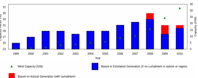
Tran 2012; Olson et al. 2014; Bird et al. 2014). Figure 1, which shows data from the U.S.
illustrates how curtailment increases as wind power capacity increases. The capacity factor,
which is the ratio of the actual output over its nameplate capacity, decreases as more wind power
is installed and subsequently curtailed.
Figure 1. Wind Capacity Factor Loss from Curtailment due to Wind Capacity Growth (Wiser et al. 2015)
Many studies have looked at the renewable energy curtailment from an economic
perspective. Some point out that the renewable curtailment is a waste of energy that leads to
economic losses for both utilities and society (Denhol & Tran, 2012). Others, however, have
concluded that, given the cost of transmission and energy storage options, renewable energy
curtailment may be a socially optimal choice (Klinge Jacobsen & Schrroder, 2012). The range of
conclusions drawn from previous studies suggests that oversupply problems in different systems
can be very distinct, suggesting that system-specific models are required to study this problem.
The financial losses associated with curtailment may depend on a number of factors, including
complex interactions between different types of generation, as well as climatic and
environmental factors, making for challenges in both characterizing the problem and solving it.
H H H H
H H H H H H H H
1999 2000 2001 2002 2003 2004 2005 2006 2007 2008 2009 2010 23 25 27 29 31 33 35 37 0 5 10 15 20 25 30 35 C a p a c it y F a c to r (% ) C a p a c it y ( G W ) Year
Based in Estimated Generation (if no curtailment in subset or region) Based on Actural Generation (with curtailment)
3
Power systems in Germany and China, as well as regional energy systems in the U.S. (e.g.,
PJM Interconnection and ERCOT (Electric Reliability Council of Texas) and MISO
(Midcontinent Independent System Operator)) have experienced generation oversupply due to
the combination of must run thermal generation and a growing penetration of renewables, in
particular wind power. Another form of generation oversupply occurs in hydropower dominated
systems, especially in situations where high levels of renewables are present (Bird et al. 2014).
Hydropower, due to its operational flexibility, is often regarded as an ideal resource to
compensate for the intermittency and unpredictability of wind power (Kern et al. 2014).
However, as more wind penetrates the electricity mix, hydroelectric dams may be limited in their
ability to accommodate wind power by reducing generation when wind is available.
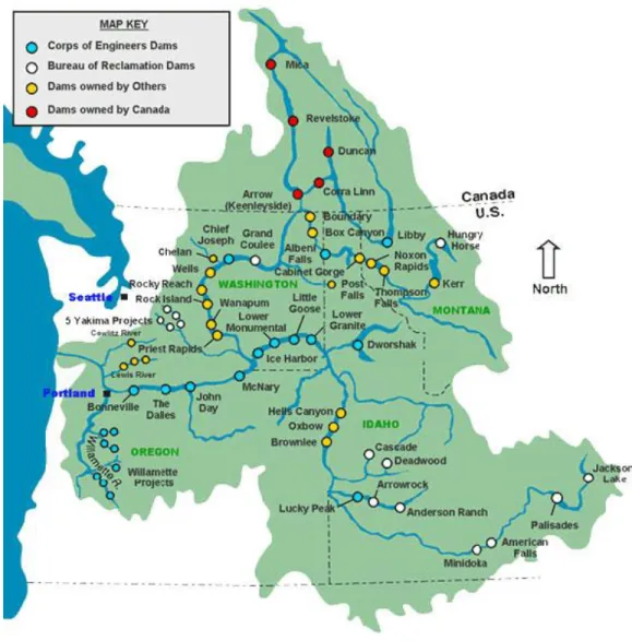
Perhaps the most prominent example of oversupply in hydropower dominated systems is
the U.S. Pacific Northwest, where hydropower meets more than 60% of regional electricity
demand, with most generation coming from the Federal Columbia River Power System (FCRPS),
a network of hydroelectric dams spanning several states. Most of the Pacific Northwest’s electric
power system is operated by Bonneville Power Administration (BPA), a federal agency that is in
charge of power plant operations, transmission, and grid balancing (BPA 2015). Within BPA’s
footprint, there are 31 federal hydroelectric dams, many additional non-federal dams, and 1
nuclear plant (BPA 2015). This system has experienced rapid growth in wind power capacity and
is already experiencing oversupply issues, with two major wind related oversupply events
occurring in 2011 and 2012.
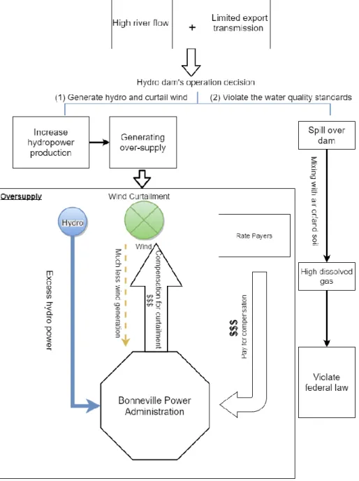
The occurrence of oversupply events and the compensation scheme is as following
(Figure 2): During high flow periods (typically summer snowmelt), hydroelectric dams in the
4
down or ramped down to their operational limits (EIA 2011; BPA 2012; Bonneville Power
Administration & Corps 2011), to maximize the use of hydropower. Nonetheless, with wind
power capacity in the region growing quickly, the combination of summer hydropower
production and wind power can create periods of regional generation over supply. During
oversupply periods, dam operators may wish to reduce hydropower production (thereby
maximizing the use of wind power) and store water for release at a later time. However, high
flow periods drive reservoir levels higher, constraining the ability of dam operators to store
additional flows. The next option available to dam operators to reduce generation is to “spill”
water (discharge it from reservoirs without generating electricity). In the FCRPS, however,
environmental regulations on flows downstream of some hydroelectric dams can obligate them
to operate in more ecologically friendly way, which can limit the dams’ ability to accommodate
high wind energy penetration. Specifically, spilling large volumes of water via spillways can
cause elevated downstream levels of total dissolved gases, primarily nitrogen (Sale 2006), and
violate federal water quality standards. Thus the combination of high reservoir levels and water
quality concerns can effectively turn dams in the FCRPS into “must run” resources that have no
choice but to generate electricity. At the same time, transmission capacity (i.e., the ability to
export excess electricity out of the region) is limited. As a result, during over supply events, it is
often wind producers in the region who ordered to shut down in order to maintain a grid balance
between supply and demand. Wind power curtailment results in the loss of revenues from wind
power generation, which is further compounded by the loss of associated renewable credits and
tax credits that producers could receive only when the generators are active. Wind producers’
losses are then compensated by BPA, and this bill is ultimately passed to all the rate payers
5
The financial losses caused by these recent oversupply events in BPA’s system (as well
as discussion of strategies for mitigating future losses) have drawn significant media attention
(Peter 2011). Wind power capacity in this region is expected to grow dramatically in coming
decades, potentially leading to more severe financially consequences from oversupply. Installed
wind capacity increased from almost 0 MW in 2000 to 4782MW by the end of 2014. An
6
(BPA, 2016). BPA has conducted a preliminary analysis of potential oversupply losses moving
forward, suggesting that annual losses could be as much as $50 million U.S. dollars (Peter 2011).
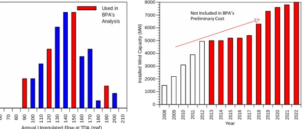
However, the analysis is limited in the following ways. First, BPA assessed potential
oversupply losses in only four, non-consecutive sample years from the historical hydrological
record, neglecting large swaths of the distribution (Figure 3) and making no effort to project
losses over longer, representative time frames. In addition, BPA’s preliminary analysis also
assumed static or very limited changes in installed wind capacity, transmission availability and
electricity prices over time. Given the projected rapid growth of wind power in the system
(Figure 4), and the uncertainty with respect to these other factors, a more comprehensive
approach is desired to understand how the challenge of managing over supply in hydropower
dominated systems like BPA’s may evolve in the future, and how transmission planning and
electricity price behavior may contribute to either lessening or worsening the problem.
To address these issues, this study uses a system-based hydro economic model, one built
specifically for the combined reservoir-power system in the Pacific Northwest, to investigate the Figure 3. BPA's preliminary analysis missed a wide
range of potential flow conditions
6 0 7 0 8 0 9 0 1 0 0 1 1 0 1 2 0 1 3 0 1 4 0 1 5 0 1 6 0 1 7 0 1 8 0 1 9 0 2 0 0 2 1 0 0 2 4 6 8 10 12 14 16 18 P ro b a b il it y ( % )
Annual Unregulated Flow at TDA (maf) Used in BPA's Analysis
Figure4. BPA's Preliminary analysis did not consider growth in wind generation capacity
2 0 0 8 2 0 0 9 2 0 1 0 2 0 11 2 0 1 2 2 0 1 3 2 0 1 4 2 0 1 5 2 0 1 6 2 0 1 7 2 0 1 8 2 0 1 9 2 0 2 0 2 0 2 1 2 0 2 2 0 1000 2000 3000 4000 5000 6000 7000 8000 In s ta lle d W in d C a p a ci ty ( M W ) Year
7
oversupply problem faced by BPA. The BPA system is evaluated dynamically to characterize the
dollar value of wind power loss from curtailment in both current and future scenarios. A
synthetic hydrologic record, based on the historical streamflow distribution, is generated to
capture a wider range of streamflow dynamics on multiple time scales. This is combined with
models of daily reservoir operations, wind generation, electricity demand and transmission
exports (mostly to California Independent System Operators), and hydropower scheduling, to
develop a probabilistic estimate of potential oversupply losses. This integrated model is then
used to assess Net Present Value (NPV) losses from oversupply over a 25-year period providing
a basis for making estimates of the value of potential mitigation strategies (e.g., construction of
additional export transmission capacity). The results of this work provide a more integrated and
improved understanding of financial losses from over supply in hydropower dominated systems,
8
CHAPTER 2: METHODS
As a federal power market administration whose system is well established and
monitored, BPA has large amounts of publicly available operating data and operates the majority
of the electricity generation and transmission capacity in the region. All data used in this study
are publicly available. Inflow data at hydropower dams in the FCRPS (Figure 5) were obtained
from BPA’s modified flow dataset. This dataset provides 80 years of river flow data (from
1928-2008) that account for factors such as withdrawals and return flows from irrigation, evaporation
and other water consumption in the region. Eight years (from 2007 to 2014) of wind, regional
electricity demand, transmission exports and thermal generation data are available from BPA’s
balancing authority website (BPA, 2015). Eighty years of daily temperature data, from 1928 and
9
2.1 Integrated Modeling
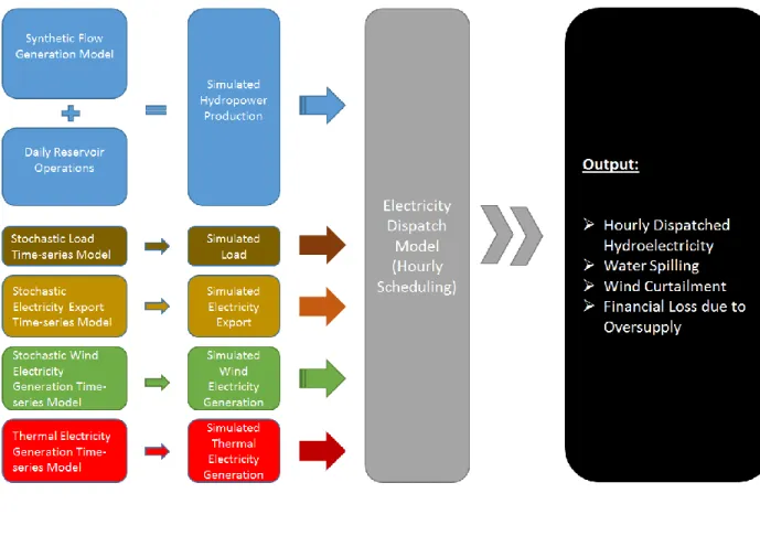
Several independent modules are integrated in order to develop the entire modelling
platform (Figure 6). Exogenous drivers of the model are simulated first (i.e., synthetic
streamflow, electricity demand, wind energy production, and transmission exports). These
simulated products then serve as inputs to the power system “decision making” process, which
includes the daily reservoir operations and hourly power scheduling models. The output of the
10
2.2 Synthetic unregulated streamflow
A primary goal of this study is to gain a more robust probabilistic understanding of the
potential for financial losses caused by oversupply events in the BPA system. Meeting this goal
requires use of an expanded hydrological dataset longer than the historical record (1928-2008).
Two main challenges exist in developing synthetic unregulated streamflow data for use in the
daily reservoir operations model. First, the synthetized streamflow has to be able to replicate
statistical characteristics of historical flows at hydroelectric dams in the FCRPS. Second, the
method must be able to generate daily values that demonstrate accurate spatial cross-correlations,
as well as temporal autocorrelations.
11
Many synthetic streamflow generation methods exist in the literature. One method that
sufficiently addresses both the aforementioned challenges is presented by Nowak et al. (2010).
This is a nonparametric stochastic approach for generation of synthetic daily flows for multiple
sites using a K-nearest neighbor (K-NN) resampling. Use of this method can be briefly
explained as follows:
1) For each site in the reservoir system, daily observed unregulated streamflow values
are converted to a proportion of the total annual flow of that particular year. This
generates P, a three-dimensional matrix (years × sites × 365). In this study, years = 81
and sites= 48.
2) A corresponding two-dimensional matrix [Z] (years × sites) is generated. Each
location (row, column) of Zis equal to the total annual flow in each year (row) at
each site (column).
3) A (1 x years) vector, zsum, is also calculated with each element equal to the total
annual unregulated streamflow across all 48 sites.
4) An theoretically unlimited number of synthetic members of zsum is then generated
(this can be done using an daily AR(1) model fit to zsum or a lag 1 K-nearest neighbor
method, as presented by Lall and Sharma (1996)). For each synthesized value, we
identify its K-nearest neighbors within historical observations of zsum, with:
K = √𝑦𝑒𝑎𝑟𝑠 (1)
Neighbors are identified within zsum as those observations that are closest to the
12
following equation, where i is the “neighbor index” with i=1 being the closest and K
is the number of nearest neighbors.
W(i) =( 1
𝑖)
∑𝐾 1/𝑖 𝑖=1
⁄ (2)
5) One of the K-nearest neighbors (a historical year y) is chosen randomly based on the
weighted resample present in equation (2). The ythrow of matrix Z isselected (zy, i.e.,
annual streamflow totals in year y for each site), as is the ythplane in P (Py, i.e., daily
flow proportions at each site in year y). A matrix of daily unregulated streamflows at
each site is then calculated by multiplying each element of zy times the vector in Py
corresponding to the same site.
2.3 Wind Power Time Series
A number of methods exist for modeling wind power production, with different methods
able to excel under different conditions and study requirements (Billinton & Chen 1996; Castino
et al. 1998; Morgan et al. 2011). For this study, an integrated representation of wind power
production in the BPA system across four temporal scales: annual, seasonal, daily and hourly
was developed. On an annual basis, the gradual increase of wind power capacity need to be
accounted for. Wind power generation in the BPA system also demonstrates strong seasonality,
with production tending to peak during from mid-summer to early fall. On a daily basis, wind
power generation demonstrates significant levels of autocorrelation; and on an hourly level, wind
power generation demonstrates a diurnal pattern (i.e. wind speed and production is higher during
13
In this study, a series of ARMA (AutoRegressive-Moving-Average) models is used to
represent these multi-scale processes and their connections. This method is able to take into
account the appropriate statistical properties of monthly and daily wind energy generation, while
maintaining similar level of autocorrelation and diurnal patterns. This approach also provides an
ability to simulate hourly wind power production conditioned on any theoretical amount of
installed wind capacity. The synthetic wind power generation method employed in this work is
described below.
First, the original dataset need to be transformed to a normalized hourly wind power
production, for a given month and year can be approximated by applying the following equation:
Normalized_Windℎ,𝑚,𝑦 =𝑂𝑏𝑠𝑒𝑟𝑣𝑒𝑑_𝑊𝑖𝑛𝑑ℎ,𝑚,𝑦− 𝑂𝑏𝑠𝑒𝑟𝑣𝑒𝑑_𝜇𝑚,𝑦
𝑂𝑏𝑠𝑒𝑟𝑣𝑒𝑑_𝜎𝑚,𝑦 (3)
Where:
h = hour of the day, ∈{1, 2, 3…24}
m = month of the year, ∈ {1, 2, 3….12}
y =sampling year, ∈ {2007, 2008…2014}
Observed_Windh,m,y = observed wind production data at hour h, month m and year y,
Observed_µm,y = the mean of all observed hourly wind production in month m and year y,
Observed_σm,y = the standard deviation of all observed wind production in month m and
year y
The above transformation generates a matrix Normalized_Windh,m,y, which is the hourly
14
Normalized_Windh,m,y contains negative numbers (i.e. low production day minus monthly
average), which need to be adjusted before log-transformation.
𝑁𝑜𝑟𝑚𝑎𝑙𝑖𝑧𝑒𝑑_𝑊𝑜𝑚𝑑′ℎ,𝑚,𝑦 = 𝑁𝑜𝑟𝑚𝑎𝑙𝑖𝑧𝑒𝑑_𝑊𝑖𝑛𝑑ℎ,𝑚,𝑦− min(𝑌𝑚) + 1 (4)
Where:
Ym = Normalized_Windm = all normalized data in month m across all years.
This adjustment makes Normalized_Wind’h,m,y a matrix that only contains positive
numbers with the minimum value of 1, enabling log transformation this leads to,
Log_Normalized_Wind’h,m,y = the log-transformed, adjusted, and normalized wind
matrix at hour h month m and year y,
Then the mean and standard deviation of all log-transformed, adjusted, and normalized
wind energy datafor each of the 8760 hours in all observed years were calculated, resulting in:
𝜇̃ = ℎ,𝑚 Log_Normalized_µ’h,m = the mean of Log_Normalized_Wind’h,m,y in hour h and
month m, across all years
𝜎̃ = ℎ,𝑚 Log_Normalized_σ’h,m= the standard deviation of Log_Normalized_Wind’h,m,y
in hour h and month m, across all years
Finally, the diurnal pattern in hourly wind power production is removed from
Log_Normalized_Wind’h,m,y by subtracting the expected hourly values and dividing by their
standard deviation. This leads to the calculation of following,
U = (LogNormalized Wind ′
15
U is a matrix of hourly wind energy data with annual capacity, seasonality (monthly
patterns) and diurnal signals removed. Next, twelve separate ARMA models are constructed, one
for each month, in order to capture the hourly statistics and time series characteristics of the
remaining signals. In this study, an ARMA(3,2), which is a combination of lag 3 autoregressive
model and a lag 2 moving average model, process was selected as the best fit for the models in
terms of autocorrelation (Figure 8). A set of optimizations are run to fit the best parameter for the
ARMA(3,2) models.
The resulting 12 monthly ARMA(3,2) models are used to simulate the hourly wind
energy data process with annual capacity, seasonality (monthly patterns), diurnal signal, over any
desired length of time, resulting in a vector called 𝐔∗. To this time series of any length, the
diurnal signal is then re-applied, the log transform is reversed, the adjustment is rescinded, and
the data is converted back to its original, non-Normal form.
Synthetic Wind = ((𝐸𝑥𝑝(𝑈∗× 𝜎̃ )+𝜇ℎ,𝑚 ̃ℎ,𝑚+ min{Y
𝑚} − 1 ) × σ𝑚,𝑀𝑊) + μ𝑚,𝑀𝑊 (6)
Where
𝜇𝑚,𝑀𝑊= mean hourly wind generation in month m, given wind capacity MW
𝜎𝑚,𝑀𝑊 = std. deviation of hourly wind generation in month m, given wind capacity
MW
In order to project the mean and standard deviation of hourly wind energy for each month
under much greater levels of installed wind capacity than what exists today in BPA’s system, we
16
capacity in BPA’s system has led to increased standard deviation of daily wind production
(Figure 7).
Figure7. Relationship between installed wind capacity and standard deviation of daily wind power generation. Figure 8 and Figure 9 show the comparison of the synthetic wind energy time series
model result against historical observations as a means of validation and the autocorrelation and
seasonality of the historical observations appears well preserved. Note that observed wind
production in Figure 9 (red line) does not have error bar. Since wind capacity in BPA’s system
has grown each year, year-on-year observed wind energy data do not provide a good direct
comparison in terms of seasonality. Thus only wind data from 2014 is used in this comparison,
providing a qualitative sense of model accuracy, albeit one that falls a little short of formal
validation. It is also important to note that, the synthetic wind energy model performs best in
terms of reproducing seasonal effects during the months most important in driving over supply in
the BPA system, i.e., June-August.
0 200 400 600 800 1000 1200 1400 1600
0 500 1000 1500 2000 2500 3000 3500 4000 4500 5000
S
ta
n
d
a
rd
D
e
v
ia
ti
o
n
o
f
D
a
ily
W
in
d
P
o
w
e
r
G
e
n
e
ra
ti
o
n
(
M
W
)
17
2.4 Temperature Modeling
Electricity demand is largely dictate d by activities that heat and cool buildings (Nawaz et
al. 2014), so daily mean temperatures are used as a primary input in simulating electricity
demand, which is synthetized via conditional resampling of the historical temperature record.
Temperature can also have direct effects on the timing of snowmelt, which is a main water
source of stream flow, thus it is important to understand and account for the observed
relationships between temperatures and streamflow patterns when generating both synthetic flow
and temperature data. To account for this, when years of flow proportions are selected (see step Figure 9. Historical and simulated wind power production seasonality
Figure 8. Historical and simulated wind power production autocorrelation B B B B B B B B
B B B
B J J J J J J J J J J J J
Jan Feb Mar Apr May Jun Jul Aug Sep Oct Nov Dec
0 500 1000 1500 2000 2500 W in d P o w e r P ro d u c ti o n ( ,W )
B Simulated J Observed
B B B B B B B B B B B B B B B B B
B B B
B J J J J J J J J J J J J J J J J J J J J J
1 2 3 4 5 6 7 8 9 10 11 12 13 14 15 16 17 18 19 20 21
0 0.1 0.2 0.3 0.4 0.5 0.6 0.7 0.8 0.9 1 A u to c u rr e la ti o n Lag (Hours)
18
#5 in the synthetic unregulated streamflow generation process), we simultaneously resample the
same year to get daily mean temperatures.
As the dominant drivers of electricity demand, temperature features prominently in most
commonly used approaches for simulating daily peak electricity demand ((Engle et al. 1992;
Bélanger & Gagnon 2002). In this study, the population weighted mean daily temperature is used
to capture the temperature effect on daily peak demand across BPA’s large geographical area.
Population and temperature data are taken from the most populated city in each of the primary
states in BPA’S footprint, namely Seattle, WA, Portland, OR, and Boise, ID. The population
weighted temperature is calculated as:
Tw𝑖 = ∑ 𝑃𝑖 ∑ 𝑃𝑖 3
𝑖=1
𝑇𝑖 (7)
Where:
Twi= Population weighted temperature
i = index for 3 different cities
Pi = Population in the indexed city
Ti = Mean daily temperature in the indexed city
2.5 Demand Modeling
The method used here to model hourly electricity demand combines hourly demand
profiles for each day of the year extracted from historical data, with a similar time series
19
First, we extract hourly demand profiles from historical electricity demand data for the
BPA system. We generate 365 hourly demand profiles in a (24 x 365) matrix S, with elements
equal to:
𝑆ℎ,𝑑 = 𝐸[𝐿ℎ,𝑑
𝐿′ℎ,𝑑] (8)
Where:
𝐿ℎ,𝑑is the demand at hour h in day d
𝐿′
𝑑 is the maximum hourly demand in day d
Hourly demand profiles are then coupled with a synthetic daily peak electricity demand
time series in order to simulate hourly demand. Similar to our approach to modeling hourly wind
power production, using historical peak electricity demand data, we remove key trends and filter
the linear process until it becomes white noise; then we re-build the time series using synthetic
records to achieve an expanded data set.
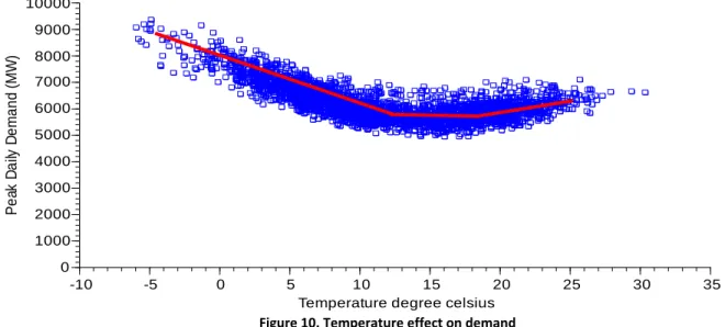
Figure 10. Temperature effect on demand
0 1000 2000 3000 4000 5000 6000 7000 8000 9000 10000
-10 -5 0 5 10 15 20 25 30 35
P
e
ak
D
a
ily
D
e
m
a
n
d
(M
W
)
20
Figure 10 shows the relationship between population weighted temperature in the BPA
system with daily peak internal electricity demand. Given coincident time series of historical
daily peak demand and population weighted temperature in the BPA system, this relationship can
then be removed. We then normalize the remaining data by subtracting its mean and dividing by
the standard deviation.
After removing the temperature effects and normalizing, the remaining process contains
non-temperature related seasonality and day of the week effects. Seasonality is removed from the
daily data by subtracting the expected daily demand and dividing by the standard deviation for
each month, and then day of the week effects are removed using similar means. The remaining
process, W, is modeled using an ARMA(3,2) model.
𝑊 =
[(𝐿𝑑,𝑚 ∗ − 𝜇
𝑑𝑚
σd𝑚 ) − 𝜇𝑑𝑜𝑤]
σ𝑑𝑜𝑤 (9)
Where:
W = daily peak demand data in MW, with effects from temperature, month and day of
week removed.
𝐿∗𝑑,𝑚 = the data with temperature effects removed
𝜇_𝑑𝑚 = the expected demand of the month m
σ_d𝑚 = the standard deviation of the month m
𝜇𝑑𝑜𝑤 = the expected demand for day-of-the-week (dow)
21
An ARMA model is then fit to time series W for simulation. After the simulation process,
the filtered signals are added back into the simulated result (W*), using a resampled time series
of population-weighted daily mean temperature.
𝐿𝑠𝑖𝑚 = ((𝑊∗σ𝑑𝑜𝑤+ 𝜇𝑑𝑜𝑤)σ_d𝑚) + 𝜇_𝑑𝑚+ 𝑓( 𝑇∗) (10)
Where:
𝐿𝑠𝑖𝑚= simulated peak demand(MW) time series
W* = ARMA generated simulated result
𝜇𝑑 is the expected demand of the weekday d
σ𝑑 is the standard deviation of the weekday d
𝑓(𝑇∗)= regression of temperature effects on peak demand
T* = synthetic population weighted daily mean temperature
After generating 𝑳𝒔𝒊𝒎 (simulated daily peak demand data), it is applied to the hourly
profiles for each calendar day taken from historical data. Figures 11 and 12 show validation of
the electricity demand model. This model did a very reasonable job of preserving both
22
2.6 Transmission Exports and Thermal Generation
Currently, the maximum export capacity for BPA is 13000 MW. Actual transmission
exports, however, are a function of demand in systems outside the BPA footprint. As such, we
model them using a similar approach as the one described in the electricity demand section (i.e.,
a function of seasonality and day of the week). Since BPA’s oversupply problem is at least partly
a byproduct of limited transmission capacity (a constrained ability to send excess electricity out Figure 12. Historical and simulated electricity demand seasonality
Figure 11. Historical and simulated electricity demand autocorrelation
B B B B B B B B B B B B J J J J J J J J J J J J
Jan Feb Mar Apr May Jun Jul Aug Sep Oct Nov Dec
4000 5000 6000 7000 8000 D e m a n d ( M W )
B Simulated J Observed
B B B B B B B
B B B
B B B B B B B B B B B J J J J J J J
J J J
J J J J
J J
J J J
J J
0 1 2 3 4 5 6 7 8 9 10 11 12 13 14 15 16 17 18 19 20
0 0.1 0.2 0.3 0.4 0.5 0.6 0.7 0.8 0.9 1 A u to c o rr e la ti o n Lag (hours)
23
of the BPA system), we also give some consideration to transmission upgrades as one potential
solution to oversupply.
The operation of individual thermal power plants is not modelled explicitly. Rather, it is
assumed that thermal generation is always available to meet any electricity demand not provided
by hydropower and wind. This is an assumption that, generally speaking, reflects how these
generators are used in the BPA system given the BPA’s ability to predict short term wind and
hydro conditions. During high flow periods, thermal generation is gradually ramped down to its
lower operational limits to accommodate the availability of wind and hydropower.
2.7 Daily Reservoir Operations (Modified HYSSR model)
24
In order to simulate the operations of dams and reservoirs in the BPA system, we use a
modified version of the Hydro System Seasonal Regulation model (HYSSR), a model designed
and built by the US Corps of Engineers. The HYSSR model is a monthly hydro-regulation model
that simulates the operation of hydroelectric dams in the Columbia River Basin. It is a
deterministic, mass-balance model that produces monthly results for reservoir storage,
hydropower production, and reservoir outflow (USACE 2008). This model has been used by
both BPA and the US Corps of Engineers for planning, operation and regulation purposes.
Since modeling oversupply events requires a time step shorter than monthly, HYSSR has
been modified to a daily model. The modified model includes the operations of 48 dams (Figure
13), which are classified as either storage or run-of-river projects. Storage projects are those that
operate based on a set of rules to regulate inflows, i.e., adjust the river’s natural flow pattern to
adapt to needs for flood control, water supply, and hydropower production. Storage projects in
the FCRPS typically capture peak runoff from spring and summer snowmelt and store it for late
summer and autumn release when the natural stream flows are lower. Run-of-river projects have
negligible storage capacity and simply pass inflows through turbines for hydro-power generation
purposes.
The modified HYSSR model calculates outflow from each project based on inflows,
minimum/maximum discharge requirements, current storage level (only applicable for storage
projects) and operational rule curves to determine each project’s end-of-day storage content,
outflow and power generation.
For storage dams, daily release decisions are governed by a set of rule curves, which are
determined based on projected inflows, flood control requirements, power generation
non-25
physical limitations (e.g., minimum outflow for environmental purposes, minimum elevation for
recreational use).
At each storage reservoir, 6 different rule curves are used in making release decisions (U.S.
Army Corps of Engineers & BPA 2011):
Critical Rule Curves (CRC) are determined annually based on the annual estimate of
system-wide electricity demand and available generation resources. These curves ensure
that each reservoir can meet its firm power production requirement even during the most
critical periods (dry periods).
Assured Refill Curves (ARC) define the reservoir elevations necessary to refill the
reservoir by July 31st each year. The ARC is calculated based on the third lowest water
year in the history, which for all projects upstream of Bonneville Dam is the period
August 1930 to July 1931.
Variable Refill Curves (VRC) define the reservoir elevations necessary to refill the
reservoirs to limit the secondary energy (non-firm requirement) production. This is
calculated based on forecasted flow of the modelling water year. In reality, VRCs are set
by dam operators probabilistically using ensemble streamflow forecasts; however, in this
study, we assume perfect foresight on the part of dam operators, which is a reasonable
assumption given that snowmelt dominated system have accurate streamflow prediction
using snowpack information, so the VRC is set based on synthetic streamflow.
Operating Rule Curve Lower Limits (ORCLL) are defined as the lowest elevation that
the modelled projects can reach. This is based on each project’s physical limitation,
26
Upper Rule Curves (URC) are set by flood control requirements, representing the
maximum elevation that projects can reach during the water year without imposing
potential flooding risks.
Operating Rule Curve (ORC) is a combination of all the above rule curves. It governs the
elevation of the projects in any given water year. It is determined as follows:
From 1 August to 31 December, ORC is the higher of ARC and CRC
From 1 January to 16 April, first define Refill Curve as the lower of the ARC and
VRC. ORC is then defined as the higher of CRC and the Refill Curve described
earlier. The ORC cannot be lower than ORCLL
Form 16 April to 31 July, same process as above except that ORCLL is no longer a
constraint.
ORC must be equal or lower than URC at all times.
Using inputs of synthetic unregulated streamflow and ORCs, the modified HYSSR model
yields daily values for reservoir storage and outflow and available hydropower production. It is
important to note that not all of the dams in BPA system are represented in HYSSR, but the
remaining dams only account for about 10% of the total hydroelectricity in this region (See the
complete dam list in Appendix A). To model this system, one key assumption made is that this
10% of dams in other areas of the BPA system produce electricity proportionally to hydropower
produced by dams in HYSSR.
2.8 Hourly scheduling model
The hourly generation scheduling model is developed to simulate the hourly operating
27
Operating and Scheduling Simulator) used by BPA and USACE (USACE 2008), those 2 models
are different. Our model takes internal demand, transmission exports, available hydropower and
thermal generation as inputs, then schedules hourly generation, with model output adhering to
the following equation:
Demand + Export = Hydro + Wind + Thermal (11)
A rolling 7-day planning horizon is used when scheduling hourly generation. This builds
in flexibility on the part of dam operators in scheduling resources to minimize spill at dams, but
it constrains their ability to incorporate future information in dam options beyond one week.
During the hourly scheduling process, the default assumption is that all available wind power is
dispatched (that is, until oversupply conditions occur). It is also assumed that during any period
in which available wind and hydropower are not sufficient to meet internal demand and export
requirements, thermal generation makes up the difference.
During oversupply periods, the hourly scheduling model displaces hydropower first.
Flow in excess of the turbine capacity is “spilled” (i.e. via non-generating spillways) until this
discharge reaches the environmental limits linked to dissolved gas entrainment. If electricity
supply is still greater than demand + exports, then thermal generation is gradually ramped down
until it reaches a minimum operating capacity (100MW), which is set empirically based on data
from BPA. A 100MW minimum thermal capacity number appears to be much lower than what
BPA used in their preliminary analysis of oversupply losses (977MW for high load hours and
852MW in low load hours), but it is supported by actual operating data published by BPA (BPA,
2015), which suggests that thermal capacity is frequently reduced well below stated guidelines.
28
its minimum capacity) wind power is curtailed to ensure the supply demand balance (Bird et al.
2014).
Spill limits at dams are the maximum flow rates at which dams can spill without violating
regulations on downstream Total Dissolved Gas (TDG) concentrations, which is mainly
dissolved nitrogen. The TDG concentration increases downstream as a function of water spilled.
Federal regulations, supported by the Endangered Species Act, set 120% TDG (meaning 120%
saturation) as the legal limit (Weitkamp, 2008) as high level of TDG can be harmful to fish.
However, historical data suggests that often during oversupply periods, dams spill water over the
127% level. Thus, in this study, we use 127% TDG as a spill limit for each dam. BPA provides
information on how to convert spill rate to downstream TDG at each dam. This makes it possible
to estimate TDG based on the spillage from dams (BPA, 2013) and determine the point at which
29
CHAPTER 3: RESULTS & DISCUSSION
3.1 Model validation
Results from the HYSSR model and the hourly scheduling model were compared against
historical observations as a measure of model validation using to the following process. First,
historical daily unregulated streamflow were input to the modified HYSSR model to simulate
reservoir releases and available hydropower production. Then the historical records of hourly
wind power production, thermal generation, transmission exports were subtracted from hourly
electricity demand for the BPA system, leaving a single hourly time series of net demand. The
hourly scheduling model was used to dispatch hydropower generation to meet this net demand,
which is not dissimilar to the manner in which hydropower is used in the system given the case
of ramping it up/down. In instances where available hydropower production, as determined by
the modified HYSSR model, was greater than net demand, remaining discharge was assumed to
be spilled (released from dams without generating electricity).
In order to validate the model, all the aforementioned historical data (unregulated streamflow,
wind power production, thermal generation, electricity demand, transmission exports, and spill at
dams) need to be available for the same time period. Unfortunately, the available data do not
always overlap in the historical record. Due to the limited data, only time period with quality
data are from September 2004 to September 2007.
The hourly scheduling model is able to reproduce historical hourly hydropower generation
30
production fall short of observed hydropower production. Another test of model accuracy comes
from comparing simulated and observed spilling; if the model is over predicting available
hydropower production, errors in simulated spilling would be evident.
Figure 15 shows simulated vs. observed spilling at all hydroelectric dams over the period
2004-2007. The model overestimates spilling in year 2005 while the estimate is fairly accurate in year
2006 (a particularly wet year). This result suggests the model may overestimate the occurrence
of oversupply events, especially in moderate or dry years. However, cumulative financial losses
of oversupply, which is the focus of this study, are driven overwhelmingly by wet years. Thus,
overestimating the frequency of small or moderate oversupply events will not greatly impact B
BB B
B BB
B BBB B
B B BB BB B B B B B B B B B B B B B B B B BBB B B B B B BB BB BB B B B B B B B B B BB B B B B BBB B B B B B B B B B B
BB BBB B B B B B B
BBB
B B BB B B B B B B B
BB B B B B BB B B
BBB B B B B B B B B B B B
BBB B B B B BB B B B B B B B B B B B B B B BBB B B B B B B B B B B B B BB B B B BB B B B B B B B B B B B B B BB B B B B B B B B B B BB B BB B B B B B BB B B B B B B B B B BB B BB B B B B B B B B B B B BB B B B B B BBB
B B BB BB B B B B B BB B B B B B B B B B B BBB B B B BB B B BB B B B B BBB
B B B BBB B B B
BBBBBB
B BB BB B B B B
BBBB B B B BB B B B B B B BB B B B
BBBBBB B B B B B B B B B B BBB B B
B BBB B B B
B BBBB B B
BBBBB B B B BB B B BB BB BB B B B
B BBB B B B
B BBBB B B B BBB B B B B B BB B B B
BBBBB B B B B B B B B B B B B BBB B B BBB B B B
B B BBB B B BB B B BBB B B B B B B B B B BB B B B B BB B B B B B B B B B B B B B B B B B B B B B B B B B B B B B B B B B B B B B B B B B BB B B B B B B B B BB BB B B B B B B B B B B B B B B BBB B B BB BBB
B B B B BB B B B B BB B B B B B B B B B B B BB B B B B B B B B
B BBBBB
B B B B B BBBBB BBB B BBBBBB B BB B BBB B BB B B B B BBB B B B BB B B B BBB B B B BB BB B B B B B B BB B B B B B B B BBB B BBBBB B
B BBB
BB B B B B B B BB B B B B BB B B B B B B B B B B B B B B B B B B B B B B B B B BBBBB B
B B B BBB B B B B B B B B B B B B B B B B B B B B B B B B B B B B B B BB BB B
B
B BBB B B B B B BB B B B
BBBB B B B B B B B B BB B B B B B BB BB B B B B B B BB B B B B
BB B B
BB B
BBB B B BB B
B B B B B B B B B B BB B B B B B B B B B B B BB B B B B B B B B B B B B B B B B BB B B B B B B BB B B B B B B BBB B B BB B B B B B B BB B B B B B BB B B B B BBB BB B B B B BB B B B B B B B B B B B B BB B B B B B BB B B B B B B B B B B B BB B B B B B BBBB B B
B BBB B BB BBB BB B B B B B B BB B B B B B B B B BB BBB B B B B B B B B B B BB B B B BBBBBB B
B
BBB B B B
B
B B BBB B B B B B B B B B B BBBBB B B B B B B B B BB B B B B B B B B B B B B
BBBBBB B BB B B B BB BB B B 0 50000 100000 150000 200000 250000 300000 350000
0 50000 100000 150000 200000 250000 300000 350000
R e a l S c h e d u le d H y d ro p o w e r (M W )
Simulated Scheduled Hydropower (MW)
0 500 1000 1500 2000 2500 3000 3500 4000 4500 5000
6/1/2004 12/1/2004 6/1/2005 12/1/2005 6/1/2006 12/1/2006 6/1/2007 12/1/2007
S p il l (K c fs ) Date Observed Spill Simulated Spill Maximun Allowed Spill
Figure 14. Hydropower generation validation
31
financial losses, relative to system drivers like installed wind capacity, electricity prices and
transmission export capacity. Model’s performance in wet years suggests that it is accurate in
estimating oversupply losses in extremely wet scenarios. Compared to a wet year, dry and
moderate years may give dam operators more flexibility for exercising their own discretion in
order to minimize oversupply events (e.g., dam operators have more room to draw down the
storage level for accommodating occasional high flows). During a wet year, however, the threat
of damaging floods makes it impossible to temporally store more water or further draw down the
reservoir, so dam operators must adhere more closely to operational rule curves, making their
decisions easier to replicate in the model.
3.2 Annual Oversupply Losses
Results suggest that under current wind capacity levels, wind producers in the BPA system experience an average curtailment of 3% of wind power production per year, with losses
occasionally reaching 20+%, typically in very wet years (Figure 16). Under scenario involving
doubled wind capacity, the average curtailment increases to 5% and the maximum possible
curtailment rises to 24% of total wind power production. Assuming the historical wind capacity
Figure 16. Annual wind power production loss
0 -3 -6 -9 -12 -15 -18 -21 -24 -27 -30
0 0.05 0.1 0.15 0.2 0.25 0.3 0.35 0.4 0.45 0.5
F
re
qu
en
cy
Wind Power Production Losses (% of total wind generation)
32
factor of 0.27 (obtained from historical data), the average 5% production loss under a scenario
involving double wind capacity would be equivalent of losing 500 MW wind power per year,
which can generate enough power for about 110,000 average US homes.
It is also important to note that as the installed wind power capacity is doubled (going
from blue to red), the distribution of losses exhibits a flatter, slightly wider distribution. This
suggests under double wind capacity it may be harder for wind producers to predict curtailment
losses on a year to year basis as the next year’s curtailment can be anywhere from the widened
distribution.
Indeed, in Figure 17, we show the distribution of financial losses (i.e., the value of
curtailed wind power production) under current and doubled wind power capacity. Financial
losses are calculated as a combination reduced of energy sales and reduced credits, namely the
U.S. Production Tax Credit and Renewable Energy Credit (both are flat rate credit). The
modeling results indicate that under current wind capacity, the expected annual loss is about $15
million, whereas the maximum potential loss can be roughly $95 million. If wind capacity is
doubled, the distribution of losses shifts to the right and demonstrates much greater variance (a
wider “tail”). Annual expected losses grow to $49 million and the maximum loss estimated to be
$212 million.
Figure 17. Distribution of annual oversupply losses
0 15 30 45 60 75 90 105 120 135 150 165 180
+ 0
0.5 1 1.5 2 2.5 3
Fr
eq
ue
nc
y
Annual Oversupply Loss (Million $)
33
Currently, in the BPA system, wind producers who experience curtailment losses are
compensated by BPA and then passed to all rate payers (Bonneville Power Administration 2016).
BPA’s annual revenue from electricity sales is about $3 – 3.5 billion based on various factors,
such as streamflow conditions, market conditions and temperatures (demand). Under the doubled
wind capacity scenario, compensating wind power producers for oversupply losses translates to
an evenly distributed rate increase (on a $/kWh basis) across all BPA consumers of as much as
4%, with an expected increase of 1%, while this value does not seem large in relative sense, the
absolute value in terms of average loss, adds over time. More importantly, the threat of large
financial disruptions, in excess of $200 million, will grow over time as installed wind capacity
increases. This suggests that as a rate payer, the electricity bill will increase as more wind
capacity is installed. For investors, this suggests that the value of the earlier wind projects can
decrease as a result of more curtailment caused by more new wind capacity installed in the area.
3.3 Comparing simulated results with BPA’s financial analysis
BPA’s own preliminary analysis suggests that the expected annual oversupply loss, given
2012 installed wind capacity, and assuming 2012 electricity prices, is $12 million with a
maximum loss of $50 million. Our own results, using the same assumptions but a more detailed
analysis involving a border set of conditions, suggests that the expected annual oversupply loss is
$15 million with a maximum loss of $96 million. The difference in the expected annual loss is
likely to be a combination of modeling bias (our model overestimates the frequency of small and
moderate oversupply events) and the modelling scope (i.e. this study uses synthetic record to
capture the entire distribution whereas BPA’s analysis only uses very limited data). The two
different modelling approaches also show a greater statistical variance in oversupply losses,
34
due in part to our use of expanded synthetic records of streamflows, wind production, and
electricity demand, which provides opportunities for the occurrence of values outside the
historical record (but within estimated maximum likelihood distributions of each variable). As
such, it seems likely that BPA has underestimated the financial losses associated with more
extreme wet weather periods, and this study’s result provides a much detailed oversupply loss
distribution under all possible conditions.
3.4 Sensitivity Analysis: Electricity Prices
Beyond hydrology and installed wind power capacity, a key driver of financial losses from
oversupply events in the BPA system is the price of electricity. The California Independent
System Operator (CAISO) is the electricity market to which BPA exports excess wind and hydro
generation (BPA 2015). Due to the heavy dependence of California generators on natural gas,
wholesale electricity prices in CAISO and thus those paid for imported power from BPA, are
strongly correlated with natural gas prices (Woo et al. 2016). This is important, because BPA’s
initial analysis of oversupply losses assumes 2012 installed wind power capacity and 2012
electricity prices. In fact, natural gas prices were near historic lows in 2012. Although gas prices
are projected to remain fairly low for the next several years (EIA 2016), BPA’s initial estimates
of financial losses from oversupply may reflect a fairly unique circumstance involving low
electricity prices. A comparison of expected annual financial losses from oversupply using the
2012 electricity price ($/MWh) as well as a distribution electricity prices, that incorporates the
wider range of natural gas prices experienced in CAISO over the last 10 years, suggests that
using the border distribution can significantly impact estimates of the mean annual oversupply
loss (Figure 18). It is notable that despite similarities in the shape of the distribution, the mean
35
full range of electricity prices, the maximum oversupply loss increased to $ 550 million
(occurring in extremely wet years with very high natural gas prices—a situation similar to that
experienced in 2006), much higher than the previous estimate of $96 million. However, when
only evaluating losses with the most recent 5 years (in which natural gas prices have been low
and relatively stable), the mean loss was estimated at $20 million with a maximum loss of $340
million.
This suggests that oversupply losses estimated with the 2012 electricity price are likely to be
substantially underpredicted, even assuming current low natural gas prices continue. That said,
with the development of improved shale gas drilling techniques (i.e. horizontal drilling and
hydraulic fracking), natural gas prices are expected to remain low and less volatile for the
foreseeable future, having a similar effect on electricity prices. As our results show, this has an
important mitigating effect on financial losses related oversupply.
Figure 18 Electricity price effect on annual oversupply loss
0 20 40 60 80 100 120 140 160 180 200
0 5 10 15 20 25 30
P
ro
b
a
b
ili
ty
(
%
)
Annual Oversupply Loss ($ Million)
Loss Based on 2012 Electricity Price
Joint Distribution With Recent 10 years Electricity Price
36
3.5 Long Term Net Present Value Loss
The net present value (NPV) of oversupply losses the BPA system was assessed over
1000 separate 25-year simulations, in order to understand these costs from a long term system
planning perspective. In particular, these could be compared with the cost of expanding
transmission capacity that could be used to export excess power. Twenty-five year NPVs were
simulated under three different wind capacity growth scenarios, low/mid/high, based on BPA’s
projections, having annual growth rates of 300/400/500 MW respectively. Gradual increases in
electricity price were also assumed as projected by EIA, 0.9% annual electricity demand growth
and a 4% discount rate. In general, the faster wind capacity is added, the greater the NPV loss
from oversupply events. Result suggest that the low-wind scenario brings about loses anywhere
from $273 million to $883 million over a 25-year period, with a mean of $529 million. The mid-
and high-wind growth scenarios resulted in similar shaped distributions for NPV losses (Figure
19) with minimum NPV losses of $368 million and $498 million, maximum losses of $1.06
billion and $1.25 billion, respectively. The expected 25-year NPV losses for the mid and high
wind growth scenarios are $681 million and $819 million respectively.
250 330 410 490 570 650 730 810 890 970 1050 1130 1210 1290 0
0.02 0.04 0.06 0.08 0.1 0.12 0.14 0.16
F
re
q
u
e
n
c
y
NPV Loss (Millions $)
Low Growth
Mid Growth
High Growth
37
3.6 Sensitivity Analysis: Transmission Upgrade
One potential solution for mitigating the impacts of oversupply events is building
additional transmission capacity to export excess electricity, in this case to California. This is an
option that has been exploited with great success in other systems experiencing oversupply
issues, with Texas being the prime example (i.e. ERCOT) (Lew et al. 2013), As such, adding
new transmission capacity has been considered seriously in the BPA system (BPA 2013).
The impacts, in terms of reducing present value oversupply loss, of adding transmission
capacity on the 25-year present value financial losses from oversupply are shown in Figure 20.
Results suggest that building a 500MW transmission line would reduce the present value loss by
$50 to $60 million over 25 years, whereas building a 1500MW transmission line would reduce
the present value oversupply loss by about $100 to $150 million. Although these savings are
significant, the cost of building transmission lines is extremely high. On average, building a
500MW transmission line costs $1-1.5 million per mile, while 1500MW transmission lines cost
$2–3 million per mile (Pletka et al. 2014).In recent years, a 215 mile 1500MW transmission line
was proposed to expand existing connections between BPA and California in order to alleviate
future oversupply issues, but this project was cancelled in 2015. The reason for cancellation,
according to Portland General Electric (PGE), the developer of this project, had to do with the
environmental impacts associated with the proposed transmission line cross a conservation area.
Based on preliminary cost estimates from Western Electricity Coordinating Council, a 215 mile
1500MW transmission line would cost $400 to $600 million. This modelling activity estimates
the avoided present value oversupply losses, with the transmission line in place, under 2012
electricity prices appears to be well below the cost of new transmission capacity even before
38
It is possible, however, that this transmission project (or one like it) may be reconsidered
by BPA in the future, and over time it’s economic viability may change. The discounting nature
of the present value calculation means that larger oversupply losses that are likely to occur out in
the future, as a result of growing wind capacity, are less impactful.
Therefore, The viability of the proposed (and now cancelled) transmission line in future
years was also tested (Figure 21), involving calculation of present value oversupply losses over
25 years beginning 15 years from now. Assuming continuous growth of wind and linear
increases in nominal electricity price (as projected by the EIA), over the next 35 years
(calculation starts in the year 2030), the 500 MW transmission upgrade project would reduce the
NPV loss by about $60 million and the 1500 MW project would reduce present value oversupply
losses by $160 to $210 million. This still falls well short of the cost of developing new
transmission capacity suggesting that such a project is unlikely to be financially attractive in the
foreseeable future.
Figure 20. Impact of transmission upgrades on present value oversupply losses, assuming transmission upgrade occurs in 2016.
250 350 450 550 650 750 850 950 1050
0 0.02 0.04 0.06 0.08 0.1 0.12
F
re
q
u
e
n
c
y
Present Value Oversupply Loss ($ Million)
Reference
500 MW additional transmission
39
3.7 Study Limitations and Future Work
This study has a number of limitations, many of which could be addressed in future work.
One key factor not considered here are changes in snowmelt timing and streamflow dynamics
that may occur as a result of climate change. The potential impacts of climate change on
streamflow in the Columbia River basin have been explored and studied (USACE & BPA 2011).
The distribution of total amount of annual precipitation may shift, leading to higher or lower
annual total streamflow. The percentage of precipitation falling as rain vs. snow may also change,
as well as the timing of snowmelt. All of this would impact the timing of high flow events that
would lead to more spilling at the dams and more oversupply related losses.
It is also worth mentioning that this work did not include consideration of the dynamic
nature of electricity pricing in the CAISO market. As demonstrated in Figure 18, the electricity
price can have a major impact on both expected and maximum oversupply losses Moreover, as
greater amounts of wind energy (or any type of renewable energy) are utilized in this market, it
650 790 930 1070 1210 1350 1490 1630 1770
0 0.02 0.04 0.06 0.08 0.1 0.12
F
re
q
u
e
n
c
y
Present Value Oversupply Loss for 2031-2055 ($ Million)
Reference
500 MW additional transmission
1500 MW additional transmission
40
could lower the wholesale electricity price, which has a direct effect on the severity of financial
losses from wind curtailment in the BPA system. Likewise, rules in CAISO for dealing with
periods of oversupply may change. Currently, the market allows prices to fall below zero to
encourage generators who can ramp down production to do so (i.e. producers need to pay
costumers to consume their electricity). However, the current minimum price (-$20/MWH) does
not impose a sufficient financial penalty on wind producers, as the combination of tax credits
(REC and PTC) pays more than $20/MWh. In recent years, CAISO has considered lowering the
negative floor to -$1000/MWh (BPA 2013), a change that could pose significantly greater losses