MULTIGRID METHODS FOR THE BIDOMAIN EQUATIONS
Yanni Lai
A dissertation submitted to the faculty at the University of North Carolina at Chapel Hill in partial fulfillment of the requirements for the degree of Doctor of Philosophy in the Department of
Mathematics in the College of Arts and Sciences.
Chapel Hill 2019
c 2019 Yanni Lai
ABSTRACT
Yanni Lai: Multigrid Methods for the Bidomain Equations (Under the direction of Boyce Griffith)
The study of cardiac electrophysiology has many applications in medical practice. One important model is the bidomain equations. In the thesis, the bidomain equations for the muscle and for the muscle and the bath are considered. By implementing multigrid algorithms as the preconditioner, we explore the block factorization approach for solving the bidomain equations.
The dissertation consists two parts, aiming to present the biological background and dis-cretization for the bidomain equations, as well as the multigrid algorithms. In the first part, we present the derivation of the formula of bidomain equations, the finite difference and finite element discretization for the bidomain system, and semi-implicit time stepping.
In the second part, we study the key facts of both geometric multigrid and algebraic multigrid method. We consider the with and without fibrosis cases. We implement the two multigrid methods as both the solver for the bidomain system and the preconditioner for the block factorization approach, and conclude that block factorization works efficiently, especially compared with the performance of the algebraic multigrid solver. We also test the block factorization with algebraic multigrid preconditioner on a realistic three-dimensional geometry, and obtain only a small increase in solver iterations as the mesh becomes finer.
ACKNOWLEDGEMENTS
First and foremost, I would like to thank my thesis advisors, Dr. Boyce Griffith, whose guidance has been indispensable for my academic studies I am especially grateful for the meaningful suggestions he made to my research, as well as his extraordinary perspective on computational mathematics, which will no doubt shape my own philosophy as I move forward.
I would like to thank my thesis committee members: Dr. Jingfang Huang, Dr. David Adalsteinsson, Dr. Katie Newhall, and Dr. Simone Rossi. Special thanks to them for the support and suggestions. Without their help, my achievements would not be possible.
I would also like to thank the tremendous support and encouragement I received from the math department at the University of North Carolina, especially from Dr. Richard McLaughlin, Dr. Laura Miller, and Ms. Laurie Straube.
I am indebted as well to my fellow students, with whom I have shared this incredible journey. Special thanks go to Dangxing Chen, Yunyan He, Fuhui Fang, Jason Pearson, Shengjie Chai, and Tianxiao Sun. I would also like to express my deep appreciation to all the wonderful faculty members and students at the University of North Carolina.
TABLE OF CONTENTS
LIST OF FIGURES . . . vii
LIST OF TABLES . . . x
LIST OF ABBREVIATIONS . . . xii
CHAPTER 1: INTRODUCTION . . . 1
1.1 Biological Background . . . 1
1.1.1 Cardiac Electrophysiology . . . 1
1.1.2 The Structure of Cardiac Muscle . . . 2
1.1.3 Cardiac Conduction System . . . 3
1.2 Discrete Cellular Models . . . 4
1.3 Continuous Models . . . 5
1.3.1 Derivation . . . 5
1.3.2 Two Forms . . . 8
1.3.3 Boundary Condition . . . 9
1.3.4 Bidomain System with Bath . . . 10
1.3.5 The Monodomain Model . . . 12
1.4 Spatial Discretization . . . 13
1.5 Time Discretization . . . 15
1.6 Solver Approaches . . . 18
CHAPTER 2: BASIC NUMERICAL METHODS FOR THE BIDOMAIN MODEL 22 2.1 Finite-Difference Spatial Discretization . . . 22
2.2 Finite-Element Spatial Discretization . . . 22
2.2.1 Bidomain Equations without Bath . . . 22
2.3 Semi-Implicit Time Stepping Method . . . 27
CHAPTER 3: MULTIGRID FOR ELLIPTIC PDES . . . 29
3.1 Classical Iterative Methods for Linear Systems . . . 29
3.1.1 Basic Idea for Multigrid Methods . . . 31
3.2 Multigrid Methods . . . 34
3.2.1 Operator Construction . . . 35
CHAPTER 4: ALGORITHMIC ASPECTS OF MULTIGRID METHODS FOR THE BIDOMAIN EQUATIONS . . . 37
4.1 Preconditioning . . . 37
4.2 Block Preconditioners . . . 38
4.3 Simulation . . . 40
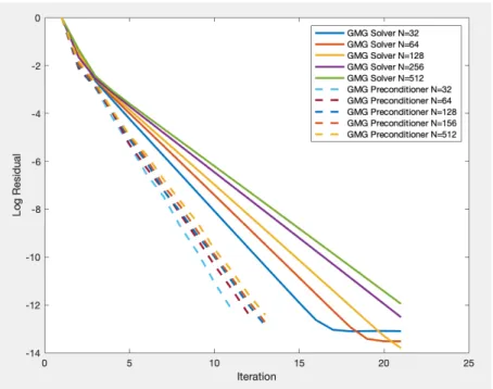
4.3.1 GMG Performance for Simple 2D Geometries . . . 40
4.3.2 AMG Performance for Simple 2D Geometries . . . 51
4.4 Conclusion . . . 64
CHAPTER 5: MG PERFORMANCE FOR REALISTIC THREE-DIMENSIONAL GEOMETRIES . . . 66
5.1 Simulation Results for Real Geometry . . . 66
5.2 Conclusion . . . 71
CHAPTER 6: CONCLUSION . . . 73
LIST OF FIGURES
1.1 Five phases of the action potential: phase 0 is upstroke, phase 1 is partial re-polarization, phase 2 is plateau, phase 3 is re-polarization, and phase 4 is resting. https://www.sciencedirect.com/topics/immunology-and-microbiology/heart-contraction . . . 2 1.2 Cardiacmyocytes have a cylindrical shape. They are connected with each other by the
intercalated disks. There are gap junctions formed of small ionic channels contained in the intercalated disks. https://courses.lumenlearning.com/austincc-ap1/chapter/cardiac-muscle-tissue . . . 3 1.3 There are five major components of the cardiac conduction system, including the SA
node, the muscular heart tissue, the AV node, the AV bundle, and the Purkinje fibers. https://courses.lumenlearning.com/suny-ap2/chapter/cardiac-muscle-and-electrical-activity . 4 1.4 Domain with a myocardium subregion (⌦m) and two bath regions (⌦b). The
bound-aries of only the myocardium are denoted as m, those of only the bath are
de-noted as b, and those between the myocardium and the bath are denoted as i.https://www.frontiersin.org/articles/10.3389/fphys.2018.01344/full . . . 10
3.1 For GMG, we use restriction operators to transfer the original problem to a coarser mesh. After solving on the coarser mesh, we transfer the residual back to the finer mesh using the interpolation operator. http://feflow.info/uploads/media/Stueben.pdf . . 34 3.2 For AMG, we ignore the geometric information when constructing the linear systems
on the "coarser" levels. http://feflow.info/uploads/media/Stueben.pdf . . . 35 3.3 Prolongation in 1D https://scholar.najah.edu/sites/default/files/all-thesis/ . . . 36
4.1 Initial condition for the bidomain system without bath using a 32⇥32 grid . . . 42 4.2 Relative residual plot for GMG solver and GMG preconditioner for GMRES with 1
for the bidomain without bath system, with t= 0.0125ms . . . 42 4.3 Solution plots at t= 1 ms, andt= 5ms (from left to right) showing V (top) and e
(bottom) . . . 43 4.4 Relative residual plot for GMG solver and GMG preconditioner for GMRES with 2
for the bidomain without bath system, with t= 0.0125ms . . . 44 4.5 Relative residual plot for GMG solver and GMG preconditioner for GMRES with 1
for the bidomain with bath system, with t= 0.0125ms . . . 46 4.6 Relative residual plot for GMG solver and GMG preconditioner for GMRES with 1
for the bidomain without bath system, with t= 0.0125ms . . . 47 4.7 Relative residual plot for block factorization approach with 1 for the bidomain with
bath system, with t= 0.0125 ms . . . 48 4.8 The existence of fibrosis (red region) forces electrical propagation to take a zigzag
4.11 Iteration plot for BGS_G/G and 1 for the bidomain without bath system, with
t= 0.0125ms and element type QUAD4 . . . 53
4.12 Solution plots at t= 1 ms of V (left) and e (right) . . . 53
4.13 Iteration plot for BGS_G/G and 1 for the bidomain without bath system, with t= 0.0125ms and element type TRI3 . . . 55
4.14 Iteration plot for BGS_G/G and 2 for the bidomain without bath system, with t= 0.0125ms, for QUAD4 (left) and TRI3 (right) . . . 56
4.15 Initial condition plot for the bidomain with bath tests . . . 56
4.16 Iteration plot for BGS_G/G and 1 for the bidomain with bath system, with t= 0.0125ms, for QUAD4 (left) and TRI3 (right) . . . 57
4.17 Solution plots at t= 1 ms of V (left), e (middle), and b (right) . . . 58
4.18 Iteration plot for BGS_G/G and 2 for the bidomain with bath system, with t= 0.0125ms, for QUAD4 (left) and TRI3 (right) . . . 59
4.19 Iteration plot or the non-aligned case with BGS_G/G and 1 for the bidomain without bath system, with t= 0.0125 ms and QUAD4 . . . 60
4.20 Iteration plot or the non-aligned case with BGS_G/G and 2 for the bidomain with bath system, with t= 0.0125 ms and QUAD4 . . . 61
4.21 Solution plots at t= 1,5,10ms (from left to right) of V (top) and e (bottom), for the non-aligned without bath case . . . 62
4.22 Solution plots of V for the the 70% fibrosis case at t= 1 ms of V of the without bath case and the with bath case . . . 64
5.1 Mesh 0(the coarsest), mesh 1, mesh 2, mesh 3, mesh4 (the finest) . . . 67
5.2 Iteration plot for BGS_G/G and 1, with t= 0.0625ms. . . 68
5.3 Iteration plot for BGS_G/G and 2, with t= 0.0625ms. . . 69
LIST OF TABLES
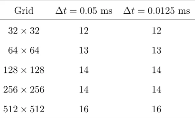
4.1 Convergence iterations for GMG as a preconditioner approach with 1for the bidomain
without bath system . . . 43 4.2 Convergence iterations for GMG as a preconditioner approach with 2for the bidomain
without bath system . . . 45 4.3 Convergence iterations for GMG as a preconditioner approach with 1for the bidomain
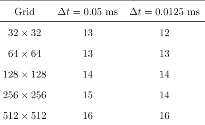
with bath system . . . 46 4.4 Convergence iterations for block factorization approach with 1 for the bidomain
without bath system . . . 47 4.5 Convergence iterations for block factorization approach with 1 for the bidomain with
bath system . . . 48 4.6 Convergence iterations for the fibrosis case with GMG as a preconditioner approach
with 1 and t= 0.0125ms for the bidomain without bath system . . . 49
4.7 Convergence iterations for the fibrosis case with GMG as a preconditioner approach with 1 and t= 0.0125ms for the bidomain with bath system . . . 50
4.8 Convergence iterations for the fibrosis case with the block factorization approach with
1 and t= 0.0125 ms for the bidomain without bath system . . . 50
4.9 Convergence iterations for the fibrosis case with the block factorization approach with
1 and t= 0.0125 ms for the bidomain with bath system . . . 51
4.10 Convergence iterations with 1 for the bidomain without bath system, with element
type QUAD4 . . . 52 4.11 Convergence iterations with 1 for the bidomain without bath system, with element
type TRI3 . . . 54 4.12 Convergence iterations for BGS_G/G with 2 for the bidomain without bath system 55
4.13 Convergence iterations for BGS_G/G with 1 for the bidomain with bath system . . 57
4.14 Convergence iterations for BGS_G/G with 2 for the bidomain with bath system . . 58
4.15 Convergence of the non-aligned case with BGS_G/G and 1 for the bidomain without
bath system, with QUAD4. . . 60 4.16 Convergence the non-aligned case with BGS_G/G and 2 for the bidomain with bath
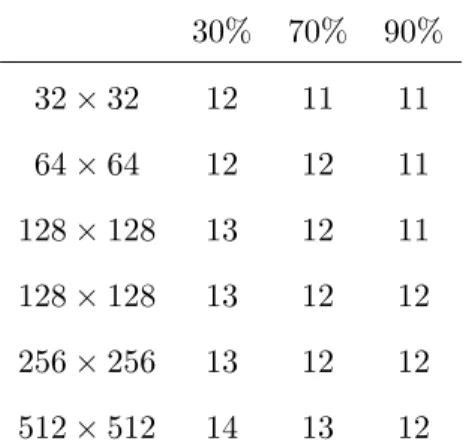
system, with QUAD4. . . 61 4.17 Convergence iterations for 30%,70%,90% fibrosis with BGS_G/G, t= 0.0125ms,
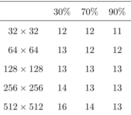
1, and QUAD4, for the without bath case . . . 63
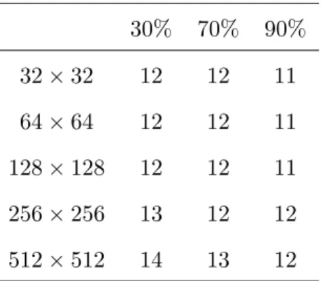
4.18 Convergence iterations for 30%,70%,90% fibrosis with BGS_G/G, t= 0.0125ms,
1, and QUAD4, for the with bath case . . . 63
5.1 Convergence iterations with 1. . . 68
5.3 Convergence iterations for30%,70%, and 90%fibrosis with BGS_G/G, t= 0.125 ms, and 1. . . 70
LIST OF ABBREVIATIONS
AMG algebraic multigrid method. 15 AV atrioventricular. 3
CG conjugate gradient method. 18
CNAB Crank-Nicolson-Adams-Bashfort. 17
FDM finite-difference method. 13 FEM finite-element method. 13 FGMRES flexible GMRES. 19
FVM finite-volume method. 13
GMG geometric multigrid method. 15
ILU incomplete LU. 18
ODE ordinary differential equations. 4
PCG preconditioned conjugate gradient. 18
SA sinoatrial. 3
CHAPTER 1 Introduction
1.1 Biological Background
1.1.1 Cardiac Electrophysiology
The study of cardiac electrophysiology is concerned with the electrical activity of the heart muscle. In a cell, the cell membrane separates its interior, which is the intracellular space, and its exterior, which is the extracellular space. Through the membrane there are proteins called ion channels. The difference in electric charge between the inside and outside of the cell across a cellular membrane is the transmembrane voltage difference. When the transmembrane voltage difference changes, the ion channels of an excitable cell can become activated, and ions can flow across the cell membrane through the channels [2]. The nearly constant transmembrane voltage difference under resting conditions is called the resting potential [3].
After re-polarization, the cell return to its resting potential [4].
Figure 1.1: Five phases of the action potential: phase 0 is upstroke, phase 1 is par-tial re-polarization, phase 2 is plateau, phase 3 is re-polarization, and phase 4 is resting. https://www.sciencedirect.com/topics/immunology-and-microbiology/heart-contraction
1.1.2 The Structure of Cardiac Muscle
In the heart, the upper chambers are called the atria, and the lower chambers are called the ventricles. The artria act as primer pumps that ensure blood flow to the ventricles, whereas the ventricles are powerful pumping chambers. The left ventricle pumps oxygenated blood from the lungs throughout the body, and the right ventricle pumps deoxygenated blood back to the lungs.
A myocyte is the spindle-shaped cell found in muscle tissue. Cardiacmyocyte is the myocyte that account for most of the mass of the atrial and ventricular muscle. A typical cardiomyocyte is approximately 100 µm in length and 10-25 µm in diameter. Cardiomyocytes have the ability to contract, which allows the heart to pump. Each cardiomyocyte’s contraction is in coordination with its neighbors. In between individual cardiomyocytes, there are intercalated disks to join them together. The gap junctions, which are small ionic channels in cylinder shape, are contained in the intercalated disks [5]. Most of the gap junctions in cardiac tissue are coupled end-to-end. Gap junctions allow the transmission of ionic currents and the spread of action potentials from cell to cell. The length of the gap junctions is about 2-12 nm, with a diameter of 2nm [6].
velocity that cardiac muscle cells send signals to heart muscle to cause it to contract [8].
The network of macromolecules in cardiac tissue is called the extracellular matrix [9]. The main structural protein in the extracellular matrix is the collagen. Cardiscyocytes are surrounded by the extracellular matrix. The extracellular matrix provides structured biochemical support around the cells, and is important for cells’ reorganization and differentiation. Collagen densities vary with tissue type. For example, in the ventricular myocardium, which is the thick middle layer of the heart wall, the density of collagen is higher compared with that in the inner and outer layers [7].
Figure 1.2: Cardiacmyocytes have a cylindrical shape. They are connected with each other by the intercalated disks. There are gap junctions formed of small ionic channels contained in the intercalated disks. https://courses.lumenlearning.com/austincc-ap1/chapter/cardiac-muscle-tissue
1.1.3 Cardiac Conduction System
Figure 1.3: There are five major components of the cardiac conduction system, including the SA node, the muscular heart tissue, the AV node, the AV bundle, and the Purkinje fibers. https://courses.lumenlearning.com/suny-ap2/chapter/cardiac-muscle-and-electrical-activity
The nodal cells refer to the cells within the SA and AV nodes. While having an action potential, these cells have no true resting potential. There are three phases for the SA nodal action potentials: the spontaneous depolarization that triggers the action potential, the depolarization of the action potential, and the re-polarization. The cycle is spontaneously repeated. The membrane potential changes in different phases corresponds primarily to the movements of calcium and potassium ions through the ion channels [10].
1.2 Discrete Cellular Models
There are two basic types of models of cardiac electrophysiology: discrete models and con-tinuous models. In discrete models, cardiac tissue is characterized based on individual cells, while in continuous models, cardiac tissue is treated as a functional syncytium (cells are linked with each other and are viewed as a whole system). Discrete models of cardiac tissue include simple cellular automaton models, coupled map lattices [11], and lattices of the system of coupled ordinary differential equations (ODE) [12].
well as the state of its neighbors. The same transition rule applies simultaneously to every cell. This kind of model is easy to implement, and is computationally inexpensive [13]. One revision of the cellular automaton models is the coupled map lattices, which involve the continuous states. The states in these models are decided by the interactions within a lattice. To allow modeling anisotropic propagation, the coupling strength of each interaction is different [14]. A further development of the previous models is to add the ODEs. With this kind of model, the detailed tissue architecture at the cell level can be modeled through the ODEs. [15]. However, this approach is computationally expensive. Also, extra information is needed to complete these models: the composition of the extracellular space, the information of cell size and capacitance, and the conductance of the gap junctions [16].
1.3 Continuous Models
In the continuous models, we view cardiac tissue as a single unit composed of electrically connected cells. The classic bidomain and monodomain models are two examples of continuous models of cardiac muscle. The bidomain system represents cardiac tissue as a functional unit comprised of intracellular and extracellular compartments. We assume the two compartments to be continuous and overlapping, and are separated by a continuous cell membrane [17].
1.3.1 Derivation
The bidomain model is based on a generalized version of Ohm’s law, which states that in a conducting body, the current density Jat a specific location is proportional to the electric fieldEat that location,
J= E, (1.3.1)
where is the conductivity of the material [18]. The electric fieldE is defined as the gradient of a scalar potential
Thus
J= r . (1.3.3)
The intracellular and extracellular current density Ji and Je are defined by:
Ji= ir i, Je= er e,
(1.3.4)
where i and e represent the intracellular and extracellular conductivity tensors respectively, and
iand e are the electrical potential in the intracellular and extracellular space. The conductivity
tensors iand e account for the anisotropy of cardiac tissue.
Assume there is no external source of charge, for a volume⌦, and denote the surface of ⌦as
. Then
ˆ
n·(Ji+Je)dS= 0. (1.3.5)
By the divergence theorem, we have
ˆ
⌦r·
(Ji+Je)d~x= 0. (1.3.6)
As the above equation should hold for all specific volumes ⌦ in the domain, thus we have
r·(Ji+Je) = 0. (1.3.7)
As a consequence of Kirchhoff’s law, any change in intracellular or extracellular current should be due to the transmembrane current (It)
Substitute Ji and Jein equations (1.3.4)to equation(1.3.8):
r·( ir i) =It, r·( er e) = It.
(1.3.9)
The transmembrane current (It) equals to the sum of a capacitive current (Ic), a resistive
current (Iion), and a stimuli applied across the membrane (Isti, take the positive to be the outward
direction) [19]
It= (Ic+Iion) Isti, (1.3.10)
where is the surface area-to-volume ratio of the cell, andIionrepresents the current flowing through
the ion channels [17]. The capacitance current is modeled by
Ic=Cm@V
@t. (1.3.11)
SubstitutingIc in(1.3.11)into(1.3.10), we have
It= (Cm
@V
@t +Iion) Isti. (1.3.12)
Equating the first equation of(1.3.9) and(1.3.12) yields the first parabolic equation of the bidomain system
(Cm
@V
@t +Iion) Isti=r·( ir i). (1.3.13)
Equating the second equation of (1.3.9) and (1.3.12) yields the second parabolic equation of the bidomain system
(Cm@V
1.3.2 Two Forms
Combine equation(1.3.13)and (1.3.14). For the applied stimuli, take the positive to be the direction into the intracellular space, andIsti in equation(1.3.13) should be positive (Ii(vol)), while
Isti in equation(1.3.14) should be negative ( Ie(vol)). The parabolic-parabolic form of the bidomain
equations is:
r·( ir i) = (Cm@V
@t +Iion(u, V)) I
(vol)
i , (1.3.15)
r·( er e) = (Cm@V
@t +Iion(u, V)) I
(vol)
e . (1.3.16)
In equation (1.3.15), u is a set of cell-level variables, such as ionic concentrations. Functional forms of Iion is obtained from specific electrophysiological cell models [20]. Equation (1.3.15) represents
the local conservation of current in the intracellular region, and equation (1.3.16) represents that in the extracellular region.
The first equation of the parabolic-elliptic form of bidomain system is equation(1.3.16), with the substitution of i=V + e. We obtain the second equation by adding equation (1.3.15)and
(1.3.16)together, such that 8 > > > > > < > > > > > :
r·( ir i) +r·( er e) =r·( ir(V + e)) +r·( er e),
(Cm@V
@t +Iion(u, V)) (Cm @V
@t +Iion(u, V)) = 0, Ii(vol) Ie(vol)= (Ii(vol)+Ie(vol)) = Itotal(vol),
(1.3.17)
where Itotal(vol) is the sum of applied stimuli. The parabolic-elliptic form is the one implemented in the numerical tests considered herein. The complete form of the parabolic-elliptic bidomain equations is
r·( ir(V + e)) = (Cm
@V
@t +Iion(u, V)) I
(vol)
i , (1.3.18)
r·(( i+ e)r e) = r·( irV) Itotal(vol). (1.3.19)
We will assume Itotal(vol) = 0, which corresponds to having Ie(vol) = Ii(vol), meaning to apply
space while simultaneously pulling the same amount out of the extracellular space [20].
The properties of equation (1.3.18) is similar to a parabolic PDE, specifically, a reaction-diffusion system. Equation (1.3.19) resembles a boundary value problem, which is an elliptic PDE.
1.3.3 Boundary Condition
To solve the bidomain model, we should add the boundary conditions. Suppose the model is defined on a volume⌦ with that at the boundary of the tissue. Similar as in section (1.3.1), letJi andJe be the intracellular and extracellular current density across the boundary respectively.
DenotingIi(surf)andIe(surf)as the intracellular and extracellular currents per unit area applied across
the boundary, we have
n·Ji=Ii(surf),
n·Je=Ie(surf),
(1.3.20)
where n denotes the outward normal to the boundary. SubstitutingJiand Je in (1.3.20) with those
in(1.3.4), the boundary conditions are
n·( ir(V + e)) =Ii(surf), (1.3.21)
1.3.4 Bidomain System with Bath
Figure 1.4: Domain with a myocardium subregion (⌦m) and two bath regions (⌦b).
The boundaries of only the myocardium are denoted as m, those of only the bath
are denoted as b, and those between the myocardium and the bath are denoted as
i.https://www.frontiersin.org/articles/10.3389/fphys.2018.01344/full
Consider adding a conductive bath besides the myocardium, and denote the bath domain as
⌦b (figure (1.4)). In this case, the transmembrane voltage V is defined on the muscle part only, the extracellular potential e in the muscle is defined on the muscle and the boundary between
muscle and bath, and the extracellular potential b in the bath is defined on the bath part and the
boundary between muscle and bath. In⌦b, the current density Jb is
Jb = br b, (1.3.23)
where b is the conductivity in the bath region.
Assume there is no external source of charge, which means that for a volume⌦b, the total
current entering it equals that leaves it. Denoting the surface of the volume as b and the outward
surface normal as n, we have that
ˆ
b
Using the divergence theorem, we have
ˆ
⌦b
r·Jbd~x= 0. (1.3.25)
As the above equation should hold for all specific volumes ⌦b in the domain, thus we have
r·Jb = 0. (1.3.26)
SubstitutingJb in equations (1.3.23)—(1.3.26), b satisfies:
r·( br b) = 0. (1.3.27)
Let idenote the boundary between muscle and bath. The boundary conditions for the muscle
part are
n·Ji=Ii(surf), on m,
n·Je=Ie(surf), on m\ i.
(1.3.28)
The boundary condition for the bath part is
n·Jb=Ib(surf), on b\ i. (1.3.29)
The boundary conditions on the boundary between the muscle and the bath are
n·Je= n·Jb, on iand
e= b, on i.
Thus the boundary conditions for the bidomain with bath problem are
n·( ir(V + e)) =Ii(surf), on m, (1.3.31)
n·( br e) =Ie(surf), on m\ i, (1.3.32)
n·( br b) =Ib(surf), on b\ i, (1.3.33)
n·( er e) = n·( br b), on i, (1.3.34)
e= b, on i. (1.3.35)
1.3.5 The Monodomain Model
Anisotropy means that the electrical properties of cardiac tissue are different in different directions. Assuming the the intracellular and extracellular regions to be equally anisotropic, we can modify the bidomain system to the monodomain system. For example, we assume the conductivity in the extracellular space to be proportional to that of the intracellular space:
e= i, (1.3.36)
with ratio . If setting Itotal(vol) to be zero as mentioned in section 1.3.2, the equation(1.3.19)can be written as
r·( ir e) = 1
1 + r·( irV). (1.3.37)
Substituting equation (1.3.37) into equation(1.3.18)withIi(vol)= 0
r·1 + ( irV) = (Cm@V
@t +Iion(u, V)). (1.3.38)
Letting = 1+ i, the final form of monodomain equation is
r·( rV) = (Cm@V
The boundary condition of this system is
n·( rV) = 0, (1.3.40)
assuming zero flux across the boundary.
From a computational standpoint, the major difference between the monodomain and bidomain equations is that the monodomain equations does not include the elliptic constraint (1.3.19). The presence of the elliptic constraint complicates the solution of the bidomain equations. From a modeling standpoint, accounting for extracellular currents, as done in the bidomain equations but not in the monodomain equations, is necessary to describe extracellular current sources, as in defibrillation, and to describe the details of current flow through electrodes.
1.4 Spatial Discretization
To discretize the Bidomain system, the finite-difference method (FDM), the finite-element method (FEM) and finite-volume method (FVM) are most commonly applied [21]. The FEM and FVM solve the weak form of the governing equations while the FDM solve the strong form. The advantage of using the weak form is that the boundary conditions can be easily imposed.
obtained the finite difference approximation, and the order of the approximation can vary according to the order of the polynomial expansion. They tested the higher order discretization scheme for the monodomain system on an idealized cubic geometry. For more complex geometries, in Sharma et al. [26], the authors solved the bidomain equations on a complex fiber geometry with the FDM. Huiskamp [27] discretized the model of the ventricle representing the myocardium of a dog using FDM. However, this creates jagged edges on curved boundaries, which influences the calculation of the boundary current flows. The advantage of FDM is the simplicity for implementation. But for irregular geometries and non-uniform meshes, FDM is difficult to apply.
The FVM considers the small volume surrounding each node point on a mesh. With this method, the volume integrals in a PDE that contains a divergence term are converted to surface integrals by applying the divergence theorem. These divergence terms are considered as fluxes at the surface of each finite volume. FVM can be easily formulated for unstructured meshes, and is popular for the bidomain and monodomain system with complex meshes. Coudiere et al. [36] analyzed the stability and convergence of FVM for the bidomain system with two time-stepping methods. A previous work [37] presented solving the bidomain equations on complex geometries with fibre rotation with FVM. In Penland et al. [38], unstructured FVM was implemented for the bidomain equations. Trew et al. [35] developed a FVM for bidomain electrical activation in discontinuous cardiac tissue. They considered modeling the cleavage planes, in which case the FVM method is desirable, since no-flux boundary conditions can be easily imposed. They mentioned that FVM has advantages over FEM for modeling cleavage planes, since FEM formulation represents cleavage planes as whole element units and thus a cleavage plane cannot have a thickness less than the mesh resolution. However, the FVM is a conservative discretization, since the flux entering a given volume is assumed to be identical to that leaving the volume.
In the numerical simulations in this thesis, I will use FDM for the geometric multigrid method (GMG) with simple two-dimensional (2D) geometries. I will use FEM for the algebraic multigrid
method (AMG) with2D and three-dimensional (3D) geometries. 1.5 Time Discretization
bidomain system considering the fiber orientation on a 3D mesh was presented. In this study, a two-step explicit method was used. The first step is to compute a new extracellular potential with the elliptic equation and the transmembrane potential at the previous time step. The second step is to apply the explicit forward-Euler method to update the transmembrane potential to the current time-step with the parabolic equation. Santos et al. [41] presented an explicit three-step scheme for solving the transmembrane potential with the parabolic PDE, and used the forward-Euler to solve for the extracellular potential. Explicit methods are easy to implement. However, they suffer a limitation in the size of time-step due to the stability issue [42].
Some research used fully implicit methods to solve the bidomain equations. In Ethier et al. [43], the propogation of electrical potential waves with the bidomain model with the ODEs was analyzed. Different implicit time-stepping methods of order 1 (backward-Euler) and 2 (implicit Gear) were presented to discretize the bidomain system. According to the research, even with very fine grids, backward-Euler can hardly provide a wave speed error below1%. It is only by reducing the time-step as small as that used for the forward-Euler, that the backward-Euler method provides accurate results. In Murillo et al. [44], the implicit backward-Euler method was implemented to solve the bidomain equations on a 2D square discretized uniformly with the FDM. Another study [45] also used the implicit second-order Gear method for the anisotropic bidomain model discretized on an unstructured grids. In addition, Munteanu and Pavarino [46] presented a parallel bidomain solver with the implicit backward-Euler method. Implicit methods have a much weaker limitation on the time-step size in terms of stability. But for bidomain equations, because they may involve a large system of nonlinear equations, the Iion term, solving the equations involves simultaneously
updating the solutions for that large system of nonlinear equations at every time-step, which is computationally expensive.
scheme, second-order Crank-Nicolson-Adams-Bashfort (CNAB) method, and third-order backward differentiation formula to the diffusion term. For the method with CNAB, the second-order Adams-Bashforth was implemented for both the ODEs and the parabolic PDEs, while Crank-Nicolson was only applied to the PDEs. For all the methods mentioned in this research, the elliptic equation was time-discretized using the forward-Euler.
Most implementations of the semi-implicit methods for the bidomain equations are first- or second-order methods [47]. In Franzonem et al. [48], the authors simulated a full normal heartbeat using the bidomain equations with ODEs. Researchers adaptively changed the time-step for different phases (the upstroke, plateau, and downstroke). The semi-implicit method in this research discretized the diffusion term by the backward-Euler method, and the non-linear reaction term was discretized by the forward-Euler method. In addition, In Whiteley’s work [49], the semi-implicit method was applied to update V and e, and the backward-Euler was applied for the ODEs. Whiteley [50]
also developed a semi-implicit scheme which allows an adaptive numerical solution in both time and space for the bidomain equations. The Crank-Nicolson-forward-Euler method, a second-order semi-implicit method, averages the current and previousV and e terms in the parabolic PDE of
the bidomain system. According to Ethier et al. [43], this method is considered accurate, as the parabolic part has a truncation error that is second-order in time. However, One disadvantage of this method is that when applying to irregular meshes, it is complicated to calculate the time-step size to satisfy the stability requirement [51].
1.6 Solver Approaches
After the time and spatial discretization, a linear systemAx=bis formed for the bidomain system, which will be shown in chapter2. In previous research, iterative solvers, geometric multigrid solvers, and algebraic multigrid solvers were applied for solving the bidomain equations.
Iterative method starts at an approximate solution. It applies to the problem repeatedly to reduce the error. Usually the stopping criterion is a value of the norm of the change in residual between two iterations. One method of this type is the conjugate gradient method (CG), which can be applied to large sparse systems that cannot be handled by direct methods. CG changes the original problem of finding the solution of a linear into an optimization problem. A further development of CG is the preconditioned conjugate gradient (PCG), which performs an additional step in CG to make the original problem well-conditioned. The performance of PCG methods depends significantly on the preconditioner applied. Generally, more expensive preconditioners lead to less iterations to achieve the desired accuracy, with higher computational cost per iteration. In Eason et al. [54], diagonal preconditioner was implemented for solving the bidomain system. One preconditioner that is widely applied is the incomplete LU (ILU), which is a sparse approximation of the LU decomposition. With this method, only parts of the original decomposed matrices are retained, and the product of the upper and lower triangular matrix will not be the exact original matrix. The ILU preconditioner was compared with diagonal preconditioner for the bidomain system in a work presented by Potse et al. [23]. According to the results, the diagonal preconditioner was much faster than ILU per iteration. However, the number of convergence iterations for the diagonal preconditioner was greater than that of ILU. Consequently, the total runtime with the diagonal preconditioner was twice greater than that with ILU.
decreases. A study [41] showed that by applying the block-Jacobi decomposition, in which case ILU is performed for the main diagonal block of the iteration matrix, PCG-ILU with a high level of fill-in was also fast when performing with parallel processors for the bidomain equations. Successive Over-Relaation (SOR) can also be used as a preconditioner for the bidomain system. SOR is a variation of the Gauss-Seidel method. It uses a parameter to overweight the correction term, and leads to a faster convergence. The symmetric SOR (SSOR) combines two SOR sweeps together, in a way that the new iteration matrix is similar to a symmetric matrix. SSOR can be shown to provide a speed-up compared with diagonal preconditioners as a bidomain equations’ preconditioner [55]. Weber dos Santos [57] showed that SSOR PCG provide a spped-up over diagonal preconditioning. Other popular preconditioners for the bidomain equations are block preconditioners. With this method, the preconditioning system is partitioned into disjoint sets of equations, and each set can be preconditioned differently. Well-known block preconditioners for the bidomain equations with CG are the block Jacobi and block SSOR methods. In Franzone et al. [48], a parallel solver with the block Jacobi PCG was applied to solve the 3D monodomain and bidomain system. Pennacchino and Simoncini [47] showed that block SSOR PCG substantially reduces the time spent to solve the linear system, without increasing the memory requirements..
For iterative solver for large sparse problem, the generalized minimal residual method (GMRES) is another common choice. In Pathmanathan et al. [20], performance of GMRES preconditioned with block Jacobi was compared with GMRES without preconditioner on the bidomain model. The authors concluded that with block Jacobi, the solving time was noticeably reduced compared with the no preconditioner case. They also considered CG, and mentioned that the difference of the performances of CG and GMRES were not significant. In Gerardo-Giorda et al. [56], in order to reduce CPU time, the researchers applied the flexible GMRES (FGMRES) and solved the preconditioner inaccurately for the monodomain and bidomain equations.
can smooth out the high frequency component of the error. The matrix transferring values from a finer level to a coarser level is the restriction matrix, while the prolongation matrix transfer values from the opposite. At each grid level except the coarsest one, iterative methods such as jacobi or Gauss-seidel are applied to reduce error. Previous studies applied MG as direct solver for the bidomain equations and obtained fast convergence [58]. In Sundnes et al. [53], the authors applied MG for bidomain system on a 2D cardiac mesh, and concluded this method to be an efficient solver. In Austin et al. [59], the black-box MG (BBMG), which is a revision of classical MG to deal with discontinuous coefficients, was implemented for test problems with discontinuities arising from inserted plunge electrodes in the heart mesh. The authors concluded that BBMG had a much faster performance compared with classical MG. MG can also be applied as the preconditioner for PCG. In Santos et al [41], the MG preconditioned CG was shown to be suited for quickly and accurately solving the bidomain system, compared with direct MG solver and CG with ILU preconditioner.
Algebraic Multigrid (AMG) is another MG method that can be applied for solving the bidomain equations. The difference between AMG an GMG is that, no information concerning the grid is required for AMG; while the coarser grids are constructed from the finer grids for GMG. By simply examining the matrix structure, the prolongation and restriction operatiors, as well as the coarser representations of the matrix are generated [55]. For unstructured meshes, AMG is useful considering the difficulties of constructing the coarser meshes. This advantage can be used when solving the bidomain equations on the real cardiac meshes, which account for the curved surface of the heart. In Austin et al. [62], the performance of AMG solver and PCG-ILU were compared for solving the elliptic component of the bidomain equations on a2D cardiac tissue. According to the results, AMG solved the problem much faster than PCG-ILU. However, since the coarser levels components should be setup for AMG, this method required a significant more memory than PCG-ILU. In addition, AMG is commonly applied as a preconditioner for solving the bidomain equations [55]. In Plank et al. [63], the performance of PCG-AMG was compared with PCG-ILU to solve the bidomain system on two3D rabbit ventricles meshes. The researchers concluded that AMG preconditioner is clearly superior to the ILU preconditioner in terms of the speed of solving. Pennacchio and Simoncini [64] applied PCG-AMG to the block form of the coefficient matrix of the bidomain system and obtained a constant growth of1 iteration until 168,577 finite element discretization elements with 12 iterations to converge to a relative tolerance of10 9. The authors’ later work [65] implemented
CHAPTER 2
Basic Numerical Methods for the Bidomain Model
2.1 Finite-Difference Spatial Discretization
In the numerical experiment with geometric multigrid methods (GMG) in2D, I use a second-order finite-difference discretization of the bidomain equations. Consider the grid-aligned case, in which case the conductivities are
i=
2 6 4 ix 0
0 iy
3 7
5, e=
2 6
4 ex 0 0 ey
3 7
5, b (2.1.1)
The bidomain with bath system is
(Cm@V
@t +Iion) I
(vol) i = ix(
@2 e
@x2 +
@2V
@x2) + iy(
@2 e
@y2 +
@2V @y2),
ix@ 2V
@x2 + iy
@2V
@y2 + ( ix+ ex)
@2 e
@x2 + ( iy+ ey)
@2 e
@y2 = I (vol) total,
b@ 2
b
@x2 + b
@2 b
@y2 = 0.
(2.1.2)
I will describe the non-aligned case in chapter 4. The spatial approximation for this system uses second-order central differences. For example, ix@
2V
i,j
@x2 + iy @2V
i,j
@y2 is approximated as
ixVi+1,j+Vix12,j 2Vi,j + iyVi,j+1+Vi,jy21 2Vi,j (2.1.3)
where x2 and y2 are the node spacing in the x and y directions. In the numerical simulation in
this thesis, I use uniform grids, in which case x= y=h. 2.2 Finite-Element Spatial Discretization
2.2.1 Bidomain Equations without Bath
term in the equations by a test function, together with the boundary conditions. Choosing the test function 2H1(⌦) and multiplying it against the strong form of the equations, we have
ˆ
⌦
Cm@V @t d~x
ˆ
⌦r·
( ir(V + e)) d~x +
ˆ
⌦
( Iion(~u, V) Ii(vol)) d~x ˆ
m
n·( ir(V + e))dS= 0, ˆ
⌦r·
( irV + ( i+ e)r e) d~x+ ˆ
⌦
Itotal(vol) d~x ˆ
m
n·( irV + ( i+ e) e)dS= 0.
(2.2.1)
To obtain a weak form of the system, we apply the integration by parts, so that
ˆ
⌦
Cm@V
@t d~x+ ˆ
⌦ ir
(V + e)r d~x +
ˆ
⌦
( Iion(~u, V) Ii(vol)) d~x ˆ
m
n·( ir(V + e)) dS= 0, ˆ
⌦ ir
Vr d~x+ ˆ
⌦
( i+ e)r er d~x+
ˆ
⌦
Itotal(vol) d~x ˆ
m
n·( irV + ( i+ e) e) dS= 0.
(2.2.2) According to boundary condition (1.3.21)and(1.3.22)we have
ˆ
m
n·( ir(V + e)) dS=Ii(surf),
ˆ
m
n·( er e) dS=Ie(surf).
(2.2.3)
The weak statement of the bidomain equations is
ˆ
⌦
Cm@V @t d~x
ˆ
⌦
( ir(V + e))r d~x+ ˆ
⌦
( Iion(~u, V) Ii(vol)) d~x ˆ
m
Ii(surf)dS= 0,
ˆ
⌦
( irV + ( i+ e)r e)r d~x+ ˆ
⌦
Itotal(vol) d~x ˆ
m
(Ie(surf)+Ii(surf))dS= 0.
(2.2.4) To obtain a numerical approximation of the weak form, we triangulate the domain into a set ofN nodes, and choose a set of basis functions 1, 2, ..., N spanning a finite-dimensional subspace
of ⌦. The basis functions used in this study satisfy an interpolation property, so that i(xj) = ij,
Lagrangian finite element basis functions. Let
V =XVi i,
e=X i i.
(2.2.5)
LetKs be the stiffness matrix for the sth subdomain,s= i, e, or b:
(Ki)jk =
ˆ
r j·( ir k)d~x,
(Kj)jk =
ˆ
r j·( jr k)d~x,
(Kb)jk =
ˆ
r j·( br k)d~x.
(2.2.6)
The discretization of the parabolic equation (1.3.18) is
CmMV˙ +KiV+Ki e+I= 0, (2.2.7)
whereV = (V1, ..., VN)and e= ( 1, ..., N)are vectors of nodal coefficients. The mass matrixMij
is
Mij =
ˆ
i jd~x, (2.2.8)
and
Ij =
ˆ
⌦
(Ii(vol)+ Iion(~u, V)) jd~x
ˆ
m
jIi(surf)dS. (2.2.9)
The discretization of the elliptic equation is
KiV+ (Ki+Ke) e+J= 0, (2.2.10)
where
ˆ
⌦
Itotal(vol) jd~x
ˆ
m
j(Ii(surf)+Ie(surf))dS=Jj = 0. (2.2.11)
Applying the assumption that Ie(vol) = Ii(vol) and Ie(surf) = Ii(surf), implying an extracellular
Since
Itotal(surf)=Ie(vol)+Ii(vol),
Itotal(surf)=Ie(surf)+Ii(surf),
(2.2.12)
we have
ˆ
⌦
Itotal(vol) jd~x
ˆ
m
Itotal(surf) jd~x=Jj = 0. (2.2.13)
2.2.2 Bidomain Equation with Bath
For the bidomain problem with a conductive bath, suppose there are two disjoint domains⌦
and⌦b , denoting the muscle and the bath, respectively. We form the first equation of the weak
form by multiplying by a test function⌫ 2H1(⌦) and integrating using the divergence theorem:
ˆ
⌦
Cm@V
@t⌫d~x ˆ
⌦
( ir(V + e))r⌫d~x+
ˆ
⌦
( Iion(~u, V) Ii(vol))⌫d~x
ˆ
m
⌫Ii(surf)dS= 0.
(2.2.14) We form the second equation of the weak form by multiplying by a test function '2H1(⌦), and integrating using the divergence theorem:
ˆ
⌦
( irV + ( i+ e)r e)r'd~x+
ˆ
⌦
Itotal(vol)'d~x ˆ
m
'(Ie(surf)+Ii(surf))dS
ˆ
m
n·( er e)'dS
ˆ
i
'(Ie(surf)+Ii(surf))dS ˆ
i
n·( er e)'dS= 0.
(2.2.15)
Applying the assumption that Ie(vol) = Ii(vol) andIe(surf)= Ii(surf)on ⌦ and m, respectively, we
have
ˆ
⌦
( irV + ( i+ e)r e)r'd~x
ˆ
m
n·( er e)'dS ˆ
i
n·( er e)'dS= 0. (2.2.16)
Recall equation (1.3.27) for b. To transfer this equation into its weak form, I multiply equation(1.3.27)and the boundary condition (1.3.33)by a test function! 2H1(⌦b),
ˆ
⌦b
r·( br b)!d~x ˆ
b
n·( br b)!dS ˆ
i
To reduce the second-order derivatives in the system, we apply the integration by parts, such that
ˆ
⌦b
br br!d~x
ˆ
b
n·( br b)!dS
ˆ
i
n·( br b)!dS= 0. (2.2.18)
According to boundary condition (1.3.33), the weak formula of the bath part is
ˆ
⌦b
br br!d~x
ˆ
b
!Ib(surf)dS ˆ
i
n·( br b)!dS= 0. (2.2.19)
Taking != on @ i, and summing equation(2.2.16)and (2.2.19), we get
ˆ
⌦
( irV + ( i+ e)r e)r'd~x+ ˆ
⌦b
br br!d~x
ˆ
b
!Ib(surf)dS
( ˆ
i
n·( br b)!dS+ ˆ
i
n·( er e)!dS) = 0.
(2.2.20)
Due to the boundary condition (1.3.34), we have
ˆ
⌦
( irV + ( i+ e)r e)r'd~x+
ˆ
⌦b
br br!d~x
ˆ
b
!Ib(surf)dS= 0. (2.2.21)
To describe the finite-element method for the bidomain with bath case, assume there are K nodes in⌦,N K nodes in i, and M nodes in⌦b. Supposex1, ..., xK are in⌦, xK+1, .., xN are in
i, andxN+1, ..., xN+M are in⌦b. The basis functions become
1, ..., K, K+1, ..., N, N+1, ..., N+M, (2.2.22)
where 1, ..., K are zero in⌦b, and N+1, ..., N+M are zero in ⌦.
For the discretization of equation(2.1.14), letV =PNj=1Vj j,and e=PNj=1 j j, indicating
thatV and eare considered only in⌦for this equation. LetV= (V1, ..., VN)and e= ( 1, ..., N).
Letting = j, j = 1, ..., N in equation(2.1.14), the discretized first equation is
where
Ij =
ˆ
⌦
(Ii(vol)+ Iion(~u, V)) jd~x
ˆ
m
jIi(surf)dS, (2.2.24)
and M is theN ⇥N mass stiffness matrix, and Ki is theN ⇥N stiffness matrix using i.
For the discretization of (2.2.21), we considerV and e in the tissue, and b in the bath, let
'= 1, ..., N and! = K+1, ..., N+M. The discretization is
N
X
k=1
(Vk
ˆ
⌦
( ir k)·r jd~x+ k
ˆ
⌦
(( i+ e)r k)·r jd~x) + NX+M
k=K+1
k(
ˆ
⌦b
( br k)·r jd~x
ˆ
b
Ib(surf) jdS) = 0,
(2.2.25) Written in matrix form, and let b = ( K+1, ..., M), the discretization is
KiV+ (Ki+Ke) e= 0,
Kb b T= 0.
(2.2.26)
where
Tj =
ˆ
b
Ib(surf) jdS. (2.2.27)
2.3 Semi-Implicit Time Stepping Method
In the numerical experiments, we use the semi-implicit time discretization. Given the time-step size t, we use the notation
8 > > > > > > > < > > > > > > > :
Vn(x) =V(x, n t),
n
e(x) = e(x, n t),
~un(x) =~u(x, n t),
n
b(x) = b(x, n t).
(2.3.1)
In equation (2.1.23), we discretize CmMV˙ as
CmM(Vn Vn 1)
In the time discretization, the diffusion term KiV+Ki e is treated implicitly as
KiVn+Ki ne. (2.3.3)
We treat the reaction termIion in equation(2.1.23)explicitly asIionn 1. We discretize equations in(2.1.26)as
KiVn+ (Ki+Ke) ne = 0,
Kb nb T= 0.
(2.3.4)
The discretized bidomain system with bath in matrix form is 2 6 6 6 6 4 Cm
t M +Ki Ki 0
Ki (1,1) (1,2)
0 (2,1) (2,2) 3 7 7 7 7 5 2 6 6 6 6 4 Vn n n b 3 7 7 7 7 5= 2 6 6 6 6 4 Cm
t MVn 1 I
0 T 3 7 7 7 7 5 (2.3.5)
where the entries in the 2by 2matrix 2 6
4(1,1) (1,2) (2,1) (2,2)
3 7
5 (2.3.6)
are
kj =
ˆ
⌦
(( i+ e)r k)·r j)d~x+
ˆ
⌦b
CHAPTER 3
Multigrid for Elliptic PDEs
3.1 Classical Iterative Methods for Linear Systems
Iterative methods use an initial guess to generate a sequence of approximated solutions, and each of the approximation is generated from the previous ones. For a linear system Ax=b, basic iterative methods usually split the Amatrix into a sum of several matrices. For example, if splitting A intoQ (Q A), we have
Qx=b+ (Q A)x. (3.1.1)
This splitting can motivate an iterative process,
Qxm =b+ (Q A)xm 1. (3.1.2)
We can initiate the iterative process with the initial value x0. We hope to be able to choose the matrixQ so that the iterative process will converge to the true solutionxwith a small number of iterations. The following three schemes are examples of commonly used classical iterative methods:
• Richardson iteration: Q=I
xm =b+ (I A)xm 1. (3.1.3)
• Jacobi iteration: Q=diag(A), denoted asD
xm=D 1(b Rxm 1), (3.1.4)
whereR=A D.
• Gauss-Seidel: Q is the strictly lower triangular part ofA, denoted as L
whereU is the strictly upper triangular part ofA, withA=L+D+U.
We can rearrange equation (3.1.2)as
xm=Q 1(Q A)xm 1+Q 1b
= (I Q 1A)xm-1+Q 1b.
(3.1.6)
For convergence analysis, subtractx= (I Q 1A)x+Q 1b fromxm= (I Q 1A)xm 1+Q 1b, we have
(xm x) = (I Q 1A)(xm 1 x). (3.1.7)
Take the norms on both sides:
||(xm x)||=||(I Q 1A)(xm 1 x)||
||(I Q 1A)||||(xm 1 x)|| ||(I Q 1A)||2||(xm 2 x)|| ...
||(I Q 1A)||m||(x0 x)||.
(3.1.8)
Thus if
lim
m!1||(I Q
1A)||m = 0. (3.1.9)
the iterative process converges. Since for any matrixM,
⇢(M)||M||. (3.1.10)
For the natural matrix norm|| · ||,where
⇢(M) =max(| 1|, ...,| n|). (3.1.11)
If
⇢(I Q 1A)<1, (3.1.12)
3.1.1 Basic Idea for Multigrid Methods
Suppose for an one dimensional elliptic equation with Dirichlet boundary
u00=f, x2(0,1) u(0) =u(1) = 0. (3.1.13)
If applying the second-order finite difference discretization
u00(xi)⇡
1
h2(ui+1 2ui+ui 1), (3.1.14)
the linear systemAu=b will be formed, where
A= 1 h2
2 6 6 6 6 6 6 6 4
2 1 0 ...
1 2 1 ... ...
... 0 1 2 3 7 7 7 7 7 7 7 5
, b= (b1, ..., bi), bi =f(xi). (3.1.15)
To calculate the eigenvalues for A, we are solving
(ui+1 2ui+ui 1)
h2 = ui, i= 1, ..., n, u0=un+1= 0. (3.1.16)
Rearranging terms
ui+1 = (2 h2 )ui ui 1. (3.1.17)
which is similar to the Chebyshev polynomials of the second kind.
U0(x) = 1,
U1(x) = 2x,
Un+1(x) = 2xUn(x) Un 1(x).
(3.1.18)
relation is
u0 = 0,
u1 = 1,
ui+1 = 2↵ui+ui 1.
(3.1.19)
Consider Uk as the kth Chebyshev polynomial of the second kind, and let↵ satisfy
uk+1 =Uk(↵),
u1 =U0(↵) = 1,
u2 =U1(↵) = 2↵u1 u0 = 2↵.
(3.1.20)
which match the form of Chebyshev polynomial of the second kind. As un+1 = 0,
Un(↵) = 0. (3.1.21)
Thus ↵ will be the root of the nth Chebyshev polynomial of the second kind. The roots are
↵k=cos
✓ k⇡ n+ 1
◆
. (3.1.22)
Plugging these into equation2↵= (2 h2 )
2cos ✓
k⇡ n+ 1
◆
= h2 k+ 2. (3.1.23)
Solving for k
k= 2 h2 1 cos ✓ k⇡ n+ 1
◆
. (3.1.24)
Using the triggonometric formula, this can be simplified to
k=
2 h2sin
2
✓ k⇡ 2(n+ 1)
◆
. (3.1.25)
In equation(3.1.25), the integerk is the frequency. Ifk in the range⇥1,12(n+ 1) , it is a low frequency; if it is in the range ⇥1
2(n+ 1), n
⇤
slowly, consider the example of Richardson iteration,
uk+1=uk+!(b Auk). (3.1.26)
The error equation is
u uk+1
=u uk !(Au Auk)
= (I !A)(u uk).
(3.1.27)
Therefore
u um= (I !A)m(u u0),
em= (I !A)me0.
(3.1.28)
To show the error decay rate for different frequency, expand e0 =u u0
e0 =
N
X
k=1
k⇠k, (3.1.29)
where⇠ are the eigenvectors ofA. Then
em = (I !A)me0 =
N
X
k=1
m,k⇠k, (3.1.30)
where
m,k = (1 ! k)m k. (3.1.31)
For the kth component, the coefficient decays with rate
| m,k||1 ! k|m| k|. (3.1.32)
Plugging in values for k,
|1 ! k|= 1
2! h2
✓
1 cos ✓
k⇡ n+ 1
◆◆
For simplicity, choose!= h42
|1 ! k|=
1 2
✓ 1 +cos
✓ k⇡ n+ 1
◆◆
. (3.1.34)
According to (3.1.34), For the low frequency case, |1 ! k|2[12,1); while for the high frequency
case, |1 ! k|2(0,12). According to this example, classical iterative methods, such as Richardson
iteration, only damp the high frequency components fast. 3.2 Multigrid Methods
The key ideas of multigrid methods (MG) are that, simple iterative methods often can be constructed to rapidly eliminate high frequency errors, and that the low-frequency component of errors on a fine mesh become high-frequency component of errors on a coarser mesh. At least for idealized problems, through transferring the error from a fine grid to a coarse grid, we can smooth out the original low-frequency component by classical iterative methods.
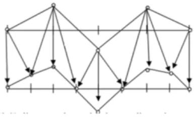
Two types of MG will be compared in this thesis, GMG and AMG. There are two types of grid transferring in MG: restriction and prolongation. The restriction operator transfers values from fine grids to coarse grids, while the prolongation operator extends data from coarse grids to fine grids. The difference between AMG and GMG are the grid transferring process. For GMG, the transferring operators are based on the geometric information (figure(3.1)).
For AMG we completely ignore the geometric information when performing the grid transferring (figure(3.2)). AMG extract all needed information from the system matrix. When the original A matrix is given, the linear systems on the "coarser" levels are automatically constructed, without the knowledge of the mesh.
Figure 3.2: For AMG, we ignore the geometric information when constructing the linear systems on the "coarser" levels. http://feflow.info/uploads/media/Stueben.pdf
3.2.1 Operator Construction
According to Briggs et al. [1], it is almost universal that the coarse grid has twice the grid spacing of the next finest grid, since using grid spacings with a ratio more than 2 provides no advantage. For most MG practice, linear interpolation, which is the simplest of the interpolation methods, is applied. Denoting the linear interpolation operator asI2hh. For one dimensional problems, it takes coarse-grid vectors and generates fine-grid vectors according toIh
2hv2h =vh, where
vh2j =vj2h,
vh2j+1 = 1 2(v
2h
j +v2j+1h ), 0j
n 2 1.
Figure 3.3: Prolongation in 1D https://scholar.najah.edu/sites/default/files/all-thesis/
In this case, at even-numbered points, the values are transferred directly from ⌦2h to ⌦h;
while at odd-numbered points, the values are the average of the adjacent coarse-grid values [1]. Writing in matrix form, it becomes
I2hhv2h = 1 2 2 6 6 6 6 6 6 6 6 6 6 6 6 6 6 6 6 6 4 1 2 1 1 2 1 1 2 1 3 7 7 7 7 7 7 7 7 7 7 7 7 7 7 7 7 7 5 2 6 6 6 6 4 v1 v2 v3 3 7 7 7 7 5 2h = 2 6 6 6 6 6 6 6 6 6 6 6 6 6 6 6 6 6 4 v1 v2 v3 v4 v5 v6 v7 3 7 7 7 7 7 7 7 7 7 7 7 7 7 7 7 7 7 5 h
=vh. (3.2.2)
For two-dimensional problems, the interpolation operator can be written as 8 > > > > > > > < > > > > > > > : vh
2i,2j =v2i,jh, for coarse grid points
vh
2i+1,2j = 12(vi,j2h+vi2+1h ,j), for points between the two coarse grid points horizontally
v2hi,2j+1 = 12(vi,j2h+vi,j2h+1), for points between the two coarse grid points vertically v2hi+1,2j+1= 14(v2i,jh+vi,j2h+1+vi,j2h+1+vi2+1h ,j+1), for points on the vertex of the square
Figure 3.4: Prolongation in 2D https://scholar.najah.edu/sites/default/files/all-thesis/
According to Briggs et al. [1], if the real error is smooth, assuming the approximation is exact at the coarse level, when this approximation is interpolated to the fine level, the interpolation is smooth, and thus we should obtain a good approximation of the error in the fine level (figure(3.5a)). However, if the real error is oscillatory, even the exact approximation of the error at the coarse level produces a not accurate approximation of the error in the fine level after the interpolation (figure (3.5b)).
Figure 3.5: (a) If the error (dots in the figure) on the coarse level is smooth, the interpolation (line connecting the dots) should give a a good approximation of the error on the fine level. (b) If the error (dots in the figure) on the coarse level is oscillatory, the interpolation (line connecting the dots) cannot give a a good approximation of the error on the fine level [1].
One common restriction operator is the full weighting operator, which is defined by
vj2h = 1 4(v
h
2j 1+ 2v2hj+v2hj+1), 1j
n
2 1. (3.2.4)
Writing in matrix form, it becomes
Ih2hvh = 1 4 2 6 6 6 6 4
1 2 1
1 2 1
1 2 1 3 7 7 7 7 5 2 6 6 6 6 6 6 6 6 6 6 6 6 6 6 6 6 6 4 v1 v2 v3 v4 v5 v6 v7 3 7 7 7 7 7 7 7 7 7 7 7 7 7 7 7 7 7 5 h = 2 6 6 6 6 4 v1 v2 v3 3 7 7 7 7 5 2h
=v2h. (3.2.5)
Figure 3.6: Restriction in1Dhttps://scholar.najah.edu/sites/default/files/all-thesis/
According to Briggs et al. [1], if choosing the full weighting restriction operator, we have
I2hh=c(I2hh)T, (3.2.6)
In2D the full weighting restriction operator can be written as
vij2h = 1 16[v
h
2i 1,2j 1+v2hi 1,2j+1+vh2i+1,2j 1+v2hi+1,2j+1
+ 2(vh2i,2j 1+v2hi,2j+1+v2hi 1,2j+vh2i+1,2j)
+ 4v2hi,2j], 1i, j n 2 1.
(3.2.7)
Figure 3.7: Restriction in2Dhttps://scholar.najah.edu/sites/default/files/all-thesis/
3.2.2 Two-grid Simple Case
MG begins with a smoothing process for the error. After the smoothing step, we reduce the high frequency components of error. To reduce the low frequency components, we apply a coarse-grid correction procedure. Once the problem on the coarser grid is solved, we interpolate the solution back to the fine grid, in order to correct the fine grid approximation of the low frequency errors.
The two-grid GMG only involves one fine level and one coarse level. Suppose the elliptic PDE after discretization on uniform grid with mesh size his
Ahuh =fh. (3.2.8)
Letukh be the approximate solution after k relaxation sweeps, the error will be
ekh=uh ukh. (3.2.9)
The steps for a two-grid GMG are
• Approximate solution uk
h by a classical iterative method
• Transfer the residual to the coarse gridrk
H =Ihhrkh
• Solve the residual equation AHekH =rkH
• Transfer the error to the fine gridekh=IHhekH
• Compute the new approximationukh+1=uk h+ekh
In practice, we usually apply1 to 3 relaxation sweeps before transferring to the next level. Relaxation on the fine grid eliminates the oscillatory components of the error, leaving the error to be smooth, which makes the interpolation work well.
3.2.3 GMG V-cycle
We can extend the two grid V-cycle to more levels. For example, in the V-cycle in figure 3.8, the GMG algorithm goes down to coarser grids(2h,4h,8h), and then back to (4h,2h, h). The algorithm is the recursive application of the following steps on each level:
Figure 3.8: Multigrid V-cycle on four levels. https://www.researchgate.net/figure/Schedule-of-grids-for-a-V-cycle-b-W-cycle-and-c-FMG-scheme-all-on-four-levels_fig10_220690328
uh Mh(uh,fh)
• Pre-smoothing: apply the smoother k times to Ahuh =fh with initial guess uh0
• If⌦h is the coarsest grid, then solve the problem
else
– Restrict the residual to the next coarser grid: r2h R2h
h (fh Ahuh)
– On the coarser gird, set initial guessu2h
– Apply the V-cycle for the next coarser grid
u2h M2h(u2h,f2h) (3.2.10)
– Update the solution with prolongation matrix: uh uh+P2hhu2h
– Post smoothing: apply the smootherk1 times to Ahuh =fh with initial guess uh0
3.3 Algebraic Multigrid for Elliptic Equations
For all MG algorithms, the fundamental components are the sequence of grids, the intergrid transferring operators, the relaxation scheme, and the solver on the coarsest grid. Different from GMG, Algebraic Multigrid (AMG) requires no explicit knowledge of the problem geometry. AMG determines coarse grids and inter-grid transfer operators based on the entries of theA matrix only. 3.3.1 Basic Idea
Suppose the one dimensional elliptic equation
u00= 0, x2⌦ (3.3.1)
is discretized on mesh (figure 3.9) with piecewise-linear finite elements.
Figure 3.9: Discretization mesh for equation (3.3.1) http://citeseerx.ist.psu.edu/viewdoc/
Choose the test function and multiplying it against the strong form of the equations, we have
ˆ xn+1
x0
u00 dx= 0. (3.3.2)
Applying integration by parts, we have
ˆ xn+1
x0
Choose a set of basis function 1, 2, ..., N (figure (3.10)), let
u=
n+1
X
i=0
ci i. (3.3.4)
Figure 3.10: Node grid xi in1D and the basis functions i https://www.geophysik.uni-muenchen.de
we have
ˆ xn+1
x0
nX+1
i=0
ci i
!0
k0dx= 0,
)
n+1
X
i=0
ci
ˆ xn+1
x0
0
i 0kdx= 0.
(3.3.5)
The entryAik in the discretization matrix is
Aik=
ˆ xn+1
x0
0
i k0dx. (3.3.6)
where
Aii=
ˆ xn+1
x0
0
i 0idx,
= ˆ xi
xi hi 1 2
0
i 0idx+
ˆ xi+hi+ 1
2
xi
0
i i0dx,
= ˆ xi
xi hi 1 2
1 hi 1
2
1 hi 1
2
dx+
ˆ xi+hi+ 1
2
xi
1 hi+1
2
1 hi+1
2
dx,
= 1 hi 1
2
+ 1 hi+1
2
, for i6= 1 or n.
(3.3.7)
Use the similar process, the ith discrete equation foru00 is
1 hi 1
2
! ui 1+
1 hi 1
2
+ 1 hi+1
2
! ui
1 hi+1
2
!
Consider another one dimensional problem with coefficients in the discrete operator
(kux)x = 0, x2⌦. (3.3.9)
If k(x) has large jumps, interpolation used in GMG can yield poor performance for this problem. We discretize this equation with piecewise-linear finite elements. The mesh is shown in figure(3.11).
Figure 3.11: Discretization mesh for equation (3.3.9)http://citeseerx.ist.psu.edu/viewdoc
In this case, the ith discrete equation for(ku
x)x is
ki 1 2
h !
ui 1+
ki 1 2
h + ki+1
2
h !
ui
ki+1 2
h !
ui+1. (3.3.10)
with eachkm with no jumps. If the grid spacing satisfyinghi 1
2 =
h ki 1
2
, and substitutehi 1
2 and
hi+1
2 in (3.2.8) as
h ki 1
2
and h ki+ 1
2
respectively, the second problem is equivalent to the first problem
ki 1 2
h !
ui 1+
ki 1 2
h + ki+1
2
h !
ui
hi+1 2
h !
ui+1 = 0,
)ui =
ki+1 2
ki+1 2 +ki
1 2
! ui 1+
ki 1 2
ki+1 2 +ki
1 2
! ui+1.
(3.3.11)
This example provides the key idea of AMG. For both of the examples, AMG only take into account the discretization matrix information, and construct the coarser levels based on these information. This resolves the problem when geometric information alone is not enough for some classes of problems, such as the second example. If considering the ith term in the discretization
matrix of the two examples