Iterative training of neural networks for intra
prediction
Thierry Dumas, Franck Galpin, and Philippe Bordes
Abstract— This paper presents an iterative training of neural networks for intra prediction in a block-based image and video codec. First, the neural networks are trained on blocks arising from the codec partitioning of images, each paired with its con-text. Then, iteratively, blocks are collected from the partitioning of images via the codec including the neural networks trained at the previous iteration, each paired with its context, and the neural networks are retrained on the new pairs. Thanks to this training, the neural networks can learn intra prediction functions that both stand out from those already in the initial codec and boost the codec in terms of rate-distortion. Moreover, the iterative process allows the design of training data cleansings essential for the neural network training. When the iteratively trained neural networks are put into H.265 (HM-16.15),−4.2%of mean BD-rate reduction is obtained, i.e. −1.8% above the state-of-the-art. By moving them into H.266 (VTM-5.0), the mean BD-rate reduction reaches −1.9%.
Index Terms—Intra prediction, neural networks, image parti-tioning.
I. INTRODUCTION
T
HE prediction of an image region from a set of pixels around this region, referred to as “context”, applies to computational photography and image editing [1], where it is known as “inpainting”, and video compression [2], where it is called “intra prediction”.The prediction of an image block from its context via a machine learning approach is made difficult by the multimodal nature of the distribution p(Y|X)of the random vector block Y given the random vector context X. For instance, let us say that a neural network is designed to predict a block from its context, and its training consists in minimizing over its parameters the l2-norm of the difference between a training block and its neural network prediction, averaged over a training set of pairs of a block and its context sampled from p(X,Y). The training assumes thatp(Y|X)is Gaussian with mean the neural network prediction. Besides, the training amounts to the maximum likelihood estimation of this mean [3]. After the training, as the prediction is the sample mean of the multimodal distribution, it looks blurry [4].
This is commonly resolved by adversarial training [5], which causes the learned model to pick a mode of p(Y|X). For inpainting, this solution is suitable as a prediction needs to be sharp and consistent with the context [6], [7], [8].
However, for intra prediction, adversarial training may be less appropriate. Indeed, a neural network trained in an
ad-The authors are with Interdigital, 975 avenue des Champs Blancs, 35576, Cesson-S´evign´e, France (e-mails: [email protected], franck. [email protected], and [email protected]).
versarial way infers a likely prediction of a block but with potentially large pixelwise differences with it [9], [10].
Instead, one can consider a classC of pairs of a block and its context defined by a known context-block relationship, then train a neural network on samples from C, hence limiting the blurriness of the neural network predictions for C. For example, in [11],C gathers the blocks provided by the H.265 partitioning [12] of images, each paired with its context. The context-block relationship is that a block of C is relatively well predicted from its reference samples by the H.265 intra prediction [13], see Figures 1 and 2, because the H.265 intra prediction drives the partitioning [14]. But, this has two drawbacks. Firstly, the neural network learns mainly the H.265 linear intra prediction. Secondly, the training set contains some pairs of a block and its context with discontinuities between the spatial distribution of pixel intensities in the block and that in its context, for which no prediction of good quality can be learned, thus hampering the training. For instance, in Figure 1, the above-mentioned discontinuities are illustrated by the diagonal dark gray border in the context not extending into the block. A neural network cannot infer this from the contextalone, see the neural network prediction in Figure 1. Likewise, in Figure 2, the above-mentioned discontinuities are represented by the horizontal border in the context tilting downward while extending into the block, instead of extending horizontally. Again, a neural network cannot infer this from the contextalone. In contrast, during the H.265 partitioning, these discontinuities are not problematic as the encoder considers both this block and its reference samples to select the best H.265 intra prediction mode in terms of rate-distortion.
To address the two drawbacks, an iterative training of neural networks for intra prediction in a block-based codec is proposed. At the first iteration, a set of neural networks is trained on samples from a class C similar to that in [11] and put into the codec as a single additional intra prediction mode. During each successive iteration, C now gathers the blocks given by the image partitioning of the codec including this single additional mode, each paired with its context, and the set of neural networks is retrained on samples from C. This way, the neural networks can learn an intra prediction progressively deviating from that in the initial codec while being beneficial in terms of rate-distortion. Moreover, from the second iteration, the pairs of a block and its context with the above-mentioned discontinuities can be detected by comparing the quality of the neural network prediction against that of the initial codec and left out of the training set.
The set of neural networks in [15] is trained iteratively with H.265 as codec, then inserted into H.265 as a single additional
Fig. 1: Prediction of a w ×w luminance block returned by the H.265 (HM-16.15) partitioning of the first frame of “BQSquare” in4:2:0with Quantization Parameter (QP) of22. At the top, a neural network trained as in [11] predicts this block from its context of decoded pixels. At the bottom, the selected H.265 mode of index25 predicts this block from its reference samples, which are made of a row of2w+1decoded pixels above this block and a column of 2w decoded pixels on its left side. w = 8. The prediction PSNRs of the neural network and the H.265 mode of index 25 are 15.82 dB and
35.46dB respectively.
mode, leading to −4.2% of mean BD-rate reduction. This improves on the state-of-the-art [11], [16] by −1.8%. When the trained neural networks are put into H.266 (VTM-5.0) as a single additional mode, the mean BD-rate reduction is−1.9%.
The contributions in this paper can be summed up as:
• We propose an iterative training of neural networks for intra prediction.
• A generic preprocessing of the context of a block and a generic postprocessing step are formulated to fit various block-based codecs, e.g. H.265 and H.266.
• A signalling of the single additional neural network-based intra prediction mode in H.266 is introduced.
II. RELATED WORK
This section presents the intra prediction in modern block-based image and video codecs. Then, it explains how some of its limitations are addressed by neural network-based methods and how our proposition falls within them.
A. Intra prediction in recent block-based codecs
Intra prediction seeks to exploit the spatial redundancies between pixels in neighboring blocks within a frame to im-prove coding efficiency. A block of pixels is inferred from the previously decoded neighborhood. The predicted block is subtracted from the original block, yielding a residue to be encoded. In H.265, for a given block to be predicted, one mode is selected among 35 fixed modes according to a rate-distortion criterion. PLANAR and DC are designed to predict the blocks with gradually varying contents. PLANAR averages a horizontal propagation of the decoded neighborhood, a.k.a reference samples, and a vertical one. DC fills the predicted block with the average of the reference samples. Each of
Fig. 2: Prediction of a w × w luminance block returned by the H.265 (HM-16.15) partitioning of the first frame of “BasketballPass” in 4:2:0 with QP= 22. At the top, a neural network trained as in [11] predicts this block from its context of decoded pixels. At the bottom, the selected H.265 mode of index12predicts this block from its reference samples.w= 8. The prediction PSNRs of the neural network and the H.265 mode of index12are 31.90dB and 37.04dB respectively.
the remaining modes propagates the reference sample values into the predicted block along a specified direction [13]. Two shortcomings of the H.265 intra prediction can be pointed out: (i) as the reference samples comprise only one row and one column of decoded pixels, see Figures 1 and 2, the intra prediction is sensitive to the quantization noise in the reference samples and cannot exploit long-range spatial dependencies,(ii)the directional model of reference samples-block dependencies does not handle complex textures.
To tackle (i) and (ii), H.266 uses respectively Multiple Reference Lines (MRL) [17] and learned modes, called Matrix Intra Prediction (MIP) [18]. More specifically, MRL allows to pick either the second row of decoded pixels above a luminance block to be predicted and the second column of decoded pixels on its left side or the fourth row and column instead of the first row and column. In MIP, the learned model of dependencies seems better adapted to complex textures as it mixes a directional propagation and a smooth variation in intensity. Each MIP mode predicts aw×hluminance block via a linear transformation of a downsampled version of the w decoded pixels above this block and theh decoded pixels on its left side. Note that, in VTM-5.0, the transformation was affine whereas, since VTM-6.0, it has been linear [19]. B. Neural network-based intra prediction
The neural network-based intra prediction offers alternative solutions to(i)and(ii). For instance, in [11], a neural network maps a context of several rows of decoded pixels above a block to be predicted and several columns on its left side to the predicted block, thus alleviating(i). As a neural network is intended as a predictor for H.265, it is trained on blocks returned by the H.265 partitioning of images, each paired with its context. Furthermore, the authors in [11] argue that overly complex textures should not appear in the training pairs. That is why, in a given image, each block for which the Mean Squared Error (MSE) between this block and its H.265 intra
prediction is too large compared to the average prediction MSE over this image is excluded from the training set. This training data cleansing differs from ours as it does not consider the quality of the neural network prediction on a candidate training block, see Section IV-E. Differently, in [15], the training set is filled with pairs of a block and its context extracted from images at random spatial locations. Each pair undergoes data augmentation. While the objective function to be minimized over the neural network parameters in [11], [15] is built from the MSE between a training block and its neural network prediction, the objective function in [20] linearly combines the same MSE-based term with an adversarial term. The objective function in [16] derives from the sum of absolute transform difference between a training block and its prediction.
The originality of [21], [22] lies in the joint training of multiple neural networks. More precisely, blocks of each size are predicted by a different set of neural networks, and the neural network training involves a partitioner and an objective function expressed as the minimum rate-distortion cost in-duced by the neural network predictions over all the partitions of each training block into sub-blocks. Consequently, the set of neural networks predicting blocks of a given size specializes in a class of textures, e.g. smooth textures for a large block size. Like this training, the iterative training emphasizes some classes of textures. However, the classes differ as an iteratively trained neural network must be a generic intra predictor, see Sections IV-B and VI-A. Note that MIP inherits from [22].
Unlike [11], [15], [16], [20], [21], [22], and our proposition where a neural network maps the context of a block to the predicted block, and the neural network predicts this block the same way on both the encoder and decoder sides of a codec, [23] splits the prediction into two parts. The neural network encoder infers from a block and its context some side information, which is sent from the encoder to the decoder. The neural network decoder computes a prediction of this block from the received side information and the context.
III. GLOBAL SETUP
The method developed in this paper aims at integrating a single additional neural network-based intra prediction mode into a block-based codec. Given that a neural network for intra prediction maps the L-shape context of a block to the predicted block, see Figure 1 and 2, fully-convolutional architectures can hardly do this mapping. As full-connections are part of the architecture, the number of neural network parameters depends on the block size. Therefore, blocks of size w×h in the codec are predicted by the neural network fh,w(.;θh,w), parametrized byθh,w, in this single additional
mode. This single additional mode thus comprises card(Q)
neural networks,Qdenoting the set of possible pairs of block height and width in the codec.
The evolution of the parameters of these neural networks from the beginning of the iterative training to the test phase is broadly depicted in Figure 3. During the training phase, at each iteration, the parameters result from the neural network trainings on pairs of a block and its context extracted from the codec partitioning of images. Between the first and second
Fig. 3: Evolution of the parameters of the neural networks belonging to the single additional neural network-based intra prediction mode throughout the proposed framework. Only two training iterations are displayed.
iterations, the single additional mode with the parameters from the first iteration is put into the codec. Between two subsequent iterations, the single additional mode updates its parameters with the parameters from the previous iteration. During the test phase, the codec with the single additional mode using the parameters from the last training iteration encodes videos. In Figure 3, the neural network architectures never change.
In details, Section IV successively justifies the iterative aspect of the training, describes the creation of the training pairs from the codec partitioning of images, and explains the motivations behind the training data cleansing popping up from the second training iteration, see the red components of Figure 3. Then, Section VI introduces the signalling of the single additional mode in the codec, which does not vary from the second training iteration to the test phase.
IV. ITERATIVE TRAINING OF NEURAL NETWORKS
This section justifies the iterative training. Some details are specified when either H.265 or H.266 is chosen as codec because they stand out as two of the most advanced video compression standards [24].
A. Modification of the training data over iterations
The first thrust of our approach is to avoid the case where a learned model gives blurry predictions because it was trained on an unrestricted variety of pairs of a block and its context in which many predictions of a block are likely given its context, cf. the multimodality discussed in Section I. That is why, first, a setΓof8-bit YCbCrimages is encoded via the codec to yield
the training sets{Sh,w}(h,w)∈R, whereSh,w contains pairs of
a luminance block of sizew×hprovided by the partitioning of an image ofΓand its context. The use ofR⊆Qinstead ofQ will be explained two paragraphs later. Then, fh,w(.;θh,w)
is trained onSh,w, see the first loop of Algorithm 1.
At this stage of the training, the learned models tend to reproduce the codec intra prediction [11]. This results from the combination of two factors. Firstly, the context fed into a neural network always includes the reference samples fed into the codec intra prediction [11], [15], [16], [25], [26], see
Algorithm 1 : iterative training.
“getPartition”, “getPartitionNN”, and Lh,w are defined by
Algorithm 2, Algorithm 3, and (1) respectively. Inputs:Γ andl∈N∗ {Sh,w}(h,w)∈R= getPartition(Γ) for all (h, w)∈R do θ(0)h,w= min θh,w Lh,w(Sh,w;θh,w)whereθh,w is randomly initialized. end for for all i∈[|1, l−1|] do {Sh,w}(h,w)∈R=getPartitionNN Γ;nθ(h,wi−1)o (h,w)∈R for all(h, w)∈R do θ(h,wi) = min θh,w Lh,w(Sh,w;θh,w)whereθh,w= θ(h,wi−1) at initialization. end for end for Output:nθ(h,wl−1)o (h,w)∈R Algorithm 2 : getPartition.
“extractPair” is detailed in Figure 5. “codec” denotes the codec of interest. Input:Γ for all (h, w)∈R do Sh,w={} end for for all I∈Γ do QP∼ U {22,27,32,37,42} ˆI, B=codec(I,QP) shuffle(B) for all(h, w)∈R do ih,w = 0 end for for all(x, y, h, w, n0, n1)∈B do if ih,w≥qthen continue end if Xc,Yc=extractPair I,ˆI, x, y, h, w, n0, n1 Sh,w.append((Xc,Yc)) ih,w += 1 end for end for Output:{Sh,w}(h,w)∈R
Figures 1 and 2, implying that this neural network can learn the codec intra prediction. Secondly, the partitioning mechanism generating the training blocks ensures that each training block is “well” predicted from its reference samples by the codec intra prediction [14], meaning that the codec intra prediction is a “good” solution to the learning problem for most of the training pairs. To allow the neural networks to learn an intra prediction progressively diverging from that in the codec while being valuable in terms of rate-distortion, for l−1 iterations,
(i)training sets are built as described above, but replacing the
Algorithm 3 : getPartitionNN
“extractPair” is explained in Figure 5. “codecNN” denotes the codec with the single additional neural network-based intra prediction mode. Inputs:Γand{θh,w}(h,w)∈R for all(h, w)∈R do Sh,w ={} end for for allI∈Γ do QP∼ U {22,27,32,37,42} ˆ I, B=codecNNI,QP;{θh,w}(h,w)∈R shuffle(B) for all (h, w)∈R do ih,w= 0 end for
for all(x, y, h, w, n0, n1, s, dnn, dc,isSplitTBs)∈Bdo
ifih,w ≥q then
continue end if
ifisSplitTBsor max(h, w)≤4 then isAdded=s==snn else isAdded=dnn≤γdc end if ifisAddedthen Xc,Yc=extractPair I,ˆI, x, y, h, w, n0, n1 Sh,w.append((Xc,Yc)) ih,w += 1 end if end for end for Output:{Sh,w}(h,w)∈R
codec by the codec with the single additional mode, (ii)the neural networks are retrained on the new training sets, see the second loop of Algorithm 1. The criterion for selecting the number of training iterationslwill be given in Section V-A1. A neural network may be needed to predict blocks of a given size in the codec but cannot be trained via Algorithm 1. This occurs when this block size exists in the intermediate steps of the partitioning, not at the output of the partition-ing. For instance, a luminance Prediction Block (PB) in an intermediate step of the H.265 partitioning can be of size either 4×4, 8×8, 16×16, 32×32 or 64×64. Therefore, Q = {(4,4),(8,8),(16,16),(32,32),(64,64)}. However, the H.265 partitioning returns luminance Transform Blocks (TBs) of sizes4×4,8×8,16×16, and 32×32exclusively. Indeed, if a 64×64 luminance PB is found at a leaf of the coding tree, the split of this PB into4 32×32TBs is forced, see the second paragraph of Section 3.2.4.1 in [27]. Thus, R = {(4,4),(8,8),(16,16),(32,32)}. In this case, each neural network predicting blocks of sizew×h,(h, w)∈Q−R, is trained on blocks extracted from images at random spatial locations, each paired with its context [15], see Section II-B.
Fig. 4: Positions of aw×hblockY and its contextX.
B. Generic intra prediction with respect to block textures The single additional neural network-based intra prediction mode should predict any texture found in the blocks of the final image partitioning. This implies that the training sets must span the variety of textures in these blocks. But, large blocks from the partitioning are usually smooth whereas small blocks exhibit unsmooth textures [28], [29], especially at small QPs. To maintain some texture diversity in each training set, the images in Γ should not all be encoded using a small QP. On the other hand, if the images inΓare all encoded using a large QP, the neural networks learn only the intra prediction from a context with large quantization noise. Therefore, the QP for encoding each image in Γ is uniformly drawn from a set of both small and large QPs, see Algorithms 2 and 3.
C. Intra prediction from a context with missing information In a block-based codec, the shape of the context of a block is constrained. For instance, in H.265 and H.266, as the blocks are processed in raster-scan order combined with Z-scan order, c.f. Sections 3.2.2 to 3.2.4 of [27] and [30], the context can only include decoded pixels located above and on the left side of the block. To comply with the constraints, the context X
takes from now on the shape in Figure 4. It comprises nl
columns of2hdecoded pixels on the left side of the blockY
andna rows ofnl+ 2wdecoded pixels above the block. As
long-range spatial dependencies between decoded pixels above and on the left side of the block are needed for prediction only in the case of a large block to be predicted, a rule for defining nl and na consists of making the ratio δ between the size
of the context and that of the block constant [15]. To keep a constant term in this ratio whatever h and w while limiting the context size, na=nl=min(h, w). Then,
δ=min(h, w) min(h, w) hw + 2 h+ 2 w .
Note that, in the case of H.265,h=w. Asna =nl=w, the
context shape in Figure 4 becomes that in [15].
More importantly, the block-based processing also causes information to be missing in the context of a block. Indeed, the n0 ∈ [|0, h|] bottommost rows and/or the n1 ∈ [|0, w|]
rightmost columns of pixels in the context may not be decoded yet, depending on the position of this block in its macro block, called Coding Tree Block (CTB) in H.265 and H.266 [13].
To overcome this, the authors in [16] first design several contexts per block size, each context containing available decoded pixels exclusively. Then, one neural network is trained per context. During the test phase, depending on the availabil-ity of the decoded pixels around a block of a given size, the context is chosen, and its associated neural network is used for prediction. But, this increases the number of neural networks in the codec, i.e. the memory cost of their parameters.
Differently, in [15], a single context is created per block size, and the missing decoded pixels are masked with the mean pixel intensity over training luminance images. Unfortunately, the mask value belongs to the range of the available decoded pixel values, leading to ambiguities between the masked portions of the context and its unmasked portions for the neural network fed with the context.
Instead, to take the mask value out of this range, the missing decoded pixels inXare first covered by a mask of value255, see the step called “mask” in Figure 5. Then, the mean µof the available decoded pixels is subtracted from them, yielding the preprocessed contextXc. Moreover,µis subtracted from
the blockY, giving rise to the preprocessed blockYc, see the
step called “center” in Figure 5.
Now that a training pair (Xc,Yc)is defined, our iterative
training can be further specified. In Algorithm 2, the encoding of an imageIofΓvia the codec returns a reconstructionˆIofI
and a setBof characteristics of each luminance block from the image partitioning. Then, for some of these luminance blocks, the block characteristics enable to create a training pair of a preprocessed block and its preprocessed context, see Figure 5. The same description goes for Algorithm 3, except that the codec is replaced by the codec with the single additional mode. D. Balancing the contributions of images to the training data If the setΓcontains YCbCrimages of various sizes and, for
each of them, the characteristics of each luminance block from the image partitioning give rise to a different training pair, the textures of the large images are more heavily represented in the training sets {Sh,w}(h,w)∈R than those of the small
images. For instance, let us focus on S16,8. The partitioning of the 1600×1200 image in Figure 6 returns 1379 8×16
luminance blocks whereas that of the480×360 image gives
158 8×16luminance blocks. This means that almost9times more training pairs inS16,8come from the1600×1200image. To avoid this, the partitioning of an image ofΓcan add at most q ∈ N∗ pairs of a preprocessed block and its preprocessed
context to each training setSh,w, see Algorithms 2 and 3.
Also to build training sets with diverse textures, for each large image inΓ, the training setSh,wshould not be filled with
the firstq w×hpreprocessed blocks coming from the top-left of this image, each paired with its preprocessed context. Thus, B is shuffled before picking from it block characteristics to create training pairs, see Algorithms 2 and 3.
E. Ignoring each training block viewed as unpredictable from its context alone
For some blocks given by the partitioning of images, the prediction of the block from its context alone via a neural
Fig. 5: Creation via “extractPair” of a pair of a w×hpreprocessed luminance block Yc and its preprocessed context Xc.
“extractPair” gathers “extract”, “mask”, and “center”. Y is extracted from the luminance channel of the first frame I of “BlowingBubbles” in4:2:0whileXis extracted from the luminance channel of its reconstructionˆIvia H.266 (VTM-5.0) with QP =37. The coordinates of the pixel at the top-left ofY inIarex= 12andy= 8.h= 8,w= 4,n0= 8, andn1= 4.
Fig. 6: Number of luminance blocks of sizes 4×8, 8× 4, 8 × 8, 8 × 16, and 16 × 8 returned by the parti-tionings of “n01440764 1063” and “n02110627 19715” in the ILSVRC2012 training RGB images [31], converted into YCbCr and4:2:0, via H.266 (VTM-5.0) with QP= 32.
network can be viewed as unfeasible, see Figures 1 and 2. If a neural network is trained on these blocks, each paired with its context, it learns to provide blurry predictions. To resolve this, these pairs must be identified and removed from the training sets. But, the identification is challenging.
A solution is to first choose a reference intra predictor that selects its prediction of a block based on both this block andsome neighboring decoded pixels. Then, a given block is labeled as unpredictable from its contextalonevia a pretrained neural network if this neural network infers from the context a prediction of low quality relatively to the prediction of the reference intra predictor. The H.265 intra prediction and that in H.266 appear to be suitable reference intra predictors as the intra prediction mode for predicting a given block is
selected on the encoder side by considering both this block and its reference samples. Based on this, the following basic criterion is derived. For a w×h luminance TB provided by the partitioning of an image of Γ, if the mean-squared error dnn∈R∗+ between the luminance TB and its neural network prediction is strictly larger than γdc, dc ∈ R∗+ denoting the third lowest mean-squared error between the luminance TB and the mode prediction over all the regular codec modes, this TB is not added to the training setSh,w. By searching for the
value ofγ∈ {0.5,1.05,1.55}yielding the best rate-distortion performance in Section V-A3,γ= 1.05was obtained.
However, the basic criterion has two downsides. Firstly, for a given luminance TB returned by the partitioning of an image, the computation of dnn and dc inside the codec increases
significantly the encoding time if this TB arises from the split of its parent PB into multiple TBs. Indeed, as the intra prediction mode is defined at the PB level, the (either H.265 or H.266) encoder runs the prediction ofeachintra prediction mode on a given luminance PB to compare them1. This implies
that, if this PB is not split into multiple TBs, there is no need to run additional predictions for calculatingdnnanddc for the
TB equivalent to its parent PB. In contrast, when a luminance PB is split into multiple TBs, the encoder does not run the prediction of each mode on a child TB2. In this case, the computation ofdnnanddc for a child TB requires additional
predictions.
To remedy to the first downside, if the luminance TB results from the split of its parent PB into multiple TBs, the basic 1For H.265, see “TEncSearch::estIntraPredLumaQT” at https: //hevc.hhi.fraunhofer.de/trac/hevc/browser/trunk/source/Lib/TLibEncoder/ TEncSearch.cpp. For H.266, see “IntraSearch::estIntraPredLumaQT” at https://vcgit.hhi.fraunhofer.de/jvet/VVCSoftware VTM/blob/master/source/ Lib/EncoderLib/IntraSearch.cpp
2For H.265, see “TEncSearch::TEncSearch::xRecurIntraCodingLumaQT” at https://hevc.hhi.fraunhofer.de/trac/hevc/browser/trunk/source/ Lib/TLibEncoder/TEncSearch.cpp. For H.266, see “In-traSearch::IntraSearch::xRecurIntraCodingLumaQT” at https://vcgit.hhi. fraunhofer.de/jvet/VVCSoftware VTM/blob/master/source/Lib/EncoderLib/ IntraSearch.cpp
criterion is replaced by another criterion that involves neither dnn nordc. More precisely, for aw×hluminance TB given
by the partitioning of an image of Γ, if the luminance TB is equivalent to its parent PB, i.e. its flag “isSplitTBs” is false, the basic criterion applies. Otherwise, the alternative criterion is that if the indexsof the intra prediction mode of the luminance TB is equal to the index snn of the single additional mode,
this TB is added to the training set Sh,w.
As a second shortcoming, the basic criterion involves pre-diction PSNRs exclusively, which incurs an adverse effect for very small luminance TBs. Indeed, when several intra prediction modes yield predictions of a luminance PB with comparable qualities, the selection of the mode for predicting this PB and its child TB(s) depends on the signalling cost of each mode. This dependency increases as this PB and its child TB(s) get smaller because the first cost involved in the selection linearly combines a distortion term and a signalling term, the former growing with the block size, unlike the latter [32], [33], [34]. As the basic criterion does not consider these signalling costs, there exist discrepancies between the small blocks in the training sets and those in the codec for which the single additional mode is likely to be selected.
Unfortunately, the solution to the first downside does not tackle the second one. Indeed, although the alternative criterion takes into account the signalling cost of each intra prediction mode, the condition on “isSplitTBs” does not guarantee that the alternative criterion systematically applies to small lumi-nance TBs. For instance, the pieces of the partitionings of the luminance channel displayed in Figure 7 via H.265 and H.266 yield many relatively small TBs that are equivalent to their parent PB, i.e. “isSplitTBs” is false. To apply the alternative criterion to all relatively small luminance TBs, the condition for picking it over the basic criterion becomes “isSplitTBs or
max (h, w)≤4”, see Algorithm 3.
V. ANALYSIS OF THE ITERATIVE TRAINING
Now that the proposed iterative training is fully detailed, the benefits of its two key features, namely its iterative aspect in Section IV-A and its training data cleansing in Section IV-E, must be assessed separately in terms of rate-distortion, see Section V-A. Then, the impact of the iterative training on the behavior of the single additional neural network-based intra prediction mode in the codec is studied, see Section V-B. A. Benefits of the two key features in terms of rate-distortion
Given that the iterative training emerges as a solution to the blurriness of the trained neural network predictions, see Section I, it must be evaluated by using an objective function that does not reduce this blurriness while being very efficient in intra prediction. Thus, the objective function Lh,w to be
minimized over the parametersθh,w offh,w(.;θh,w)is built
on the l2-norm of the difference between a w×hblock and its neural network prediction. Moreover, regularization via l2 -norm of the neural network weights Wh,w applies [35].
L(Sh,w;θh,w) = 1 card(Sh,w) X (Xc,Yc)∈Sh,w Yc− ˆ Yc 2 +λkWh,wk22 (1)
Fig. 7: Partitioning of the first64×64block of the luminance channel of the first frame of “BasketballPass” in 4:2:0 via H.265 (HM-16.15) with (a) QP = 22 and (b) QP = 37 and H.266 (VTM-5.0) with (c) QP= 22and (d) QP= 37.
where Yˆc = fh,w(Xc;θh,w) and λ = 0.0005. Γ gathers
the ILSVRC2012 [31] and DIV2K [36] training RGB images converted into YCbCr. AsΓcontains nearly1.3×106images
and it is observed experimentally that around20×106 pairs per training set prevents overfitting, the maximum number q of pairs the partitioning of an image brings to each training set, see Algorithms 2 and 3, is fixed to20.
As this paper does not address the neural network archi-tectures, the experiments reuse the neural networks architec-tures in [15]. More precisely, the neural network predicting w×h blocks with min (h, w) ≤ 8 is made of four fully-connected layers. Each layer excluding the last one has 1200
output neurons. The last layer has hw output neurons. The neural network predictingw×hblocks withmin (h, w)>8
takes the convolutional architecture in [15] with a stack of4
convolutional layers for each of the two rectangular portions of the context in Figure 4, a channelwise fully-connected layer, and a stack of 4 transpose convolutional layers. The number of output feature maps in the 4 convolutional layers are respectively 64,64, 128, and128. The number of output feature maps in the 4 transpose convolutional layers are respectively128,64,64, and1. In all architectures, each layer apart from the last one has LeakyReLU with 0.1 as slope. Please refer to Table XIII (c) and (d) in [15] to know the stride and the kernel size in each layer of the convolutional architecture. Given the above description and Figure 4, the four neural networks predicting blocks of sizes4×4,8×8,
16×16, and 32×32contain respectively2998816,3344464,
1339072, and3802816parameters. Moreover, the distributions for initializing the neural network parameters and the training hyperparameters in [15] are re-used. The training involves Tensorflow 1.9.0 [37] and a GPU NVIDIA Tesla P100.
Up to now, only the training phase of the neural networks has been covered. For the following experiments, details on the test phase must be specified. During the test phase, for a given w×hblock to be predicted, the preprocessing of its context and the postprocessing of the neural network prediction derive from the context preprocessing during the training phase. A single step is added to adjust to the codec internal bitdepth b ∈ {8,10}. More specifically, the context X of this block is divided by 2b−8 and preprocessed as described by “mask” and “center” in Figure 5, yielding the preprocessed contextXt
c.
Then, the neural network prediction is postprocessed by adding the meanµof the available decoded pixels inX, multiplying by 2b−8, and clipping to
0,2b−1
, yielding the prediction
ˆ Y=min max 2b−8 fh,w Xtc;θh,w +µ ,0 ,2b−1 . Section V-A uses H.265 (HM-16.15). The signalling of the single additional mode in H.265 follows [15]. H.265 with the single additional mode is denoted H.265-ITNN, ITNN standing for Iteratively Trained Neural Networks. The test set gathers luminance images only as the neural networks are trained on pairs of a luminance block and its context and, to simplify the interpretation of the results, the intra prediction of chrominance blocks is temporarily set aside. Therefore, H.265-ITNN and H.265 encode the luminance channel of the first frame of video sequences from the Common Test Conditions (CTC) [38]. Note that the neural networks cannot specialize to the CTC video sequences as they do not belong to Γ. The rate-distortion performance is computed via the Bjontegaard metric [39] of H.265-ITNN with respect to H.265 with QP∈ {17,22,27,32,37,42}.
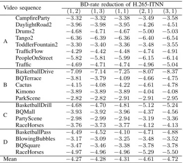
1) Benefits of the iterative aspect: To avoid mixing up the contributions of the iterative aspect and the training data cleansing to the rate-distortion performance, the BD-rate re-ductions in Table I are computed by eliminating the training data cleansing from the iterative training. This means that Algorithm 3 becomes Algorithm 2, but substituting “codec” with “codecNN”.
The second training iteration yields −0.30% of additional mean BD-rate reduction with respect to the first one. From the second iteration to the third one, −0.11% of additional mean BD-rate reduction is obtained, see the last three columns of Table I. The benefits of the iterative training come from a change in the training data, not an underfitting at the first iteration. This is proved by two experimental pieces of evidence. Firstly, when l = 1 and the number of training iterations at each stage of the learning rate scheduling is multiplied by p∈ {2,3}, almost no change in the mean BD-rate reduction is reported with respect to the case l= 1 and p = 1, see the first three columns of Table I. Yet, the case l = 1 andp = 3 and the case l = 3 andp = 1 amount to the same number of training iterations. Besides, we have run the case l = 3 and p= 1 with the random initialization of the neural network parameters at each iteration. This means
TABLE I: BD-rate reductions in % of H.265-ITNN after each iteration of the iterative training without the training data cleansing. The anchor is H.265 (HM-16.15). Only the luminance channel of the first frame of each video sequence is considered.(l, p)refers to the training usingliterations and, at each iteration, multiplying byp∈N∗the number of training iterations at each stage of the learning rate scheduling.
Video sequence (1,2)BD-rate reduction of H.265-ITNN(1,3) (1,1) (2,1) (3,1)
A CampfireParty −3.32 −3.32 −3.38 −3.49 −3.58 DaylightRoad2 −3.96 −3.98 −3.95 −4.26 −4.51 Drums2 −4.68 −4.71 −4.67 −5.00 −5.03 Tango2 −6.36 −6.39 −6.36 −6.40 −6.54 ToddlerFountain2 −3.30 −3.40 −3.36 −3.48 −3.55 TrafficFlow −4.29 −4.42 −4.48 −4.74 −4.91 PeopleOnStreet −5.82 −5.81 −5.99 −6.15 −6.14 Traffic −4.69 −4.71 −4.74 −4.96 −5.04 B BasketballDrive −7.09 −7.14 −7.25 −8.07 −8.37 BQTerrace −3.81 −3.79 −4.09 −4.66 −4.75 Cactus −4.15 −4.08 −4.22 −4.61 −4.78 Kimono −3.89 −3.89 −3.89 −4.04 −4.08 ParkScene −2.82 −2.82 −2.91 −2.91 −2.95 C BasketballDrill −4.68 −4.70 −4.81 −5.12 −5.24 BQMall −3.93 −3.92 −3.96 −4.37 −4.56 PartyScene −2.98 −2.99 −2.94 −3.19 −3.36 RaceHorses −3.76 −3.73 −3.77 −4.12 −4.13 D BasketballPass −4.49 −4.52 −4.10 −4.71 −4.88 BlowingBubbles −3.17 −3.09 −3.25 −3.48 −3.52 BQSquare −3.47 −3.46 −3.38 −3.78 −3.78 RaceHorses −4.97 −4.96 −4.96 −5.29 −5.50 Mean −4.27 −4.28 −4.31 −4.61 −4.72
that, in Algorithm 1, the random initialization of the first minimization applies to all subsequent minimizations. In this case, negligible variations in BD-rate reductions with respect to those in the last column of Table I have been observed.
When a fourth training iteration was run, −0.02% of additional mean BD-rate reduction with respect to the third iteration was obtained. As the rate-distortion benefit of the fourth training iteration is viewed as small compared to those of the first three iterations,l= 3 in Sections V-B and VII.
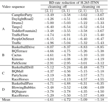
2) Benefits of the training data cleansing: Table II shows that, forl= 2andp= 1,−0.48%of additional mean BD-rate reduction is reported when the training data cleansing is turned on with respect to the case where it is turned off. For l= 3
and p = 1, the additional mean BD-rate reduction reaches −0.46%. Therefore, the iterative aspect and the training data cleansing have equally large rate-distortion impacts.
3) Cumulated benefits: Overall, the iterative training yields −0.87% of additional mean BD-rate reduction compared to a single-step training, see the third column of Table I and the last column of Table II.
4) Influence of the training QPs: The experiments in Sec-tion V-A1 have also been re-run by replacing the set of QPs in Algorithms 2 and 3 with {17,24}. The mean BD-rate reduction for l= 3with{17,24} as set of QPs is smaller in absolute value than that with{22,27,32,37,42}as set of QPs by nearly0.03. When re-running the experiments by replacing the set of QPs in Algorithms 2 and 3 with{35,40}, the mean BD-rate reduction for l = 3 with {35,40} as set of QPs is smaller in absolute value than that with{22,27,32,37,42}as set of QPs by0.40. This validates the choice of the set of both small and large QPs in Algorithms 2 and 3.
TABLE II: BD-rate reductions in%of H.265-ITNN when the training data cleansing is turned off and on. The anchor is H.265 (HM-16.15). Only the luminance channel of the first frame of each video sequence is considered.
Video sequence
BD-rate reduction of H.265-ITNN cleansing off cleansing on
(2,1) (3,1) (2,1) (3,1) A CampfireParty −3.49 −3.58 −3.62 −3.67 DaylightRoad2 −4.26 −4.51 −4.66 −4.63 Drums2 −5.00 −5.03 −5.22 −5.33 Tango2 −6.40 −6.54 −6.52 −6.54 ToddlerFountain2 −3.48 −3.55 −3.58 −3.67 TrafficFlow −4.74 −4.91 −5.21 −5.40 PeopleOnStreet −6.15 −6.14 −6.40 −6.47 Traffic −4.96 −5.04 −5.32 −5.43 B BasketballDrive −8.07 −8.37 −8.83 −8.85 BQTerrace −4.66 −4.75 −5.26 −5.38 Cactus −4.61 −4.78 −5.10 −5.10 Kimono −4.04 −4.08 −4.20 −4.19 ParkScene −2.91 −2.95 −3.01 −3.12 C BasketballDrill −5.12 −5.24 −6.48 −6.73 BQMall −4.37 −4.56 −5.15 −5.18 PartyScene −3.19 −3.36 −3.57 −3.71 RaceHorses −4.12 −4.13 −4.57 −4.55 D BasketballPass −4.71 −4.88 −6.31 −6.35 BlowingBubbles −3.48 −3.52 −4.06 −4.09 BQSquare −3.78 −3.78 −4.35 −4.50 RaceHorses −5.29 −5.50 −5.57 −5.89 Mean −4.61 −4.72 −5.09 −5.18
B. Behavior of the modified codec through iterations
The rate-distortion benefits identified in Section V-A3 lead to the question of how the iterative training affects the codec with the single additional mode.
To answer this, let us first analyze how the neural network prediction evolves over iterations. This analysis requires to predict a given block from its context via a neural network after two different training iterations. But, within H.265-ITNN, the quantization noise in the context of this block varies over iterations as the codec intra prediction changes over iterations, making the predictions incomparable. That is why the first analysis is not performed inside H.265-ITNN. Instead, the following experiment acts as a substitute. Triplets of a w×w block, its context, and its reference samples are extracted from the luminance channel of YCbCr images at random spatial
locations. These images are obtained by converting into YCbCr
the24RGB images in the Kodak suite [40] and the100RGB images in the BSDS test dataset [41]. Then, for each triplet, the two predictions of the block given by the neural network fw,w
.;θ(w,wi) after the first and third training iterations, i.e. i ∈ {0,2}, are compared to the prediction of the best H.265 intra prediction mode in terms of prediction PSNR.
Successful cases for the iterative training, i.e. with improve-ment of the quality of the neural network prediction over iterations, are illustrated by Figures 8, 10, and 12. Failure cases are depicted in Figures 9, 11, and 13. In all cases, the neural network prediction gets shaper over iterations. Note that this indicates that the training data cleansing reaches its goal. In Figure 9, the predicted block given by the neural network after the first iteration and the one from the best H.265 mode are all black. But, after the third iteration, the bottom-right of the predicted block returned by the neural network
(a)
(b) (c)
(d)
(e) (f)
Fig. 8: Predictions of a 4×4 luminance block: (a) context, (b) prediction from the context via the neural network after the first training iteration (PSNR= 23.74dB), (c) prediction via the neural network after the third iteration (PSNR= 30.44
dB), (d) reference samples, (e) prediction from the reference samples via the best H.265 mode of index 30 in terms of prediction PSNR (PSNR= 28.79dB), and (f) original block.
(a)
(b) (c)
(d)
(e) (f)
Fig. 9: Predictions of a 4×4 luminance block: (a) context, (b) prediction from the context via the neural network after the first training iteration (PSNR= 33.60dB), (c) prediction via the neural network after the third iteration (PSNR= 30.66
dB), (d) reference samples, (e) prediction from the reference samples via the best H.265 mode of index 10 in terms of prediction PSNR (PSNR= 38.30dB), and (f) original block.
contains an extrapolation of the diagonal bright gray border at the top-right of the context. In Figure 11, the predicted block provided by the neural network after the first iteration and the one from the best H.265 mode are all dark gray. However, after the third iteration, we see at the bottom-right of the predicted block generated by the neural network an extrapolation of the diagonal bright gray border at the bottom of the context. Similarly, in Figure 13, the predicted block computed by the neural network after the first iteration looks blurry whereas, after the third iteration, it includes a black triangle, which contrasts with the predicted block from the best H.265 mode. According to the last three examples, the neural network can diverge from the best H.265 mode over iterations. Note that this suggests that the iterative aspect of the training actually achieves its target. Differently, in Figures 8 and 12, the predicted block given by the neural network comes closer to the one from the best H.265 mode over iterations. This convergence might stem from the very high likelihood of the best H.265 mode given the context of the block.
Given the conclusions of the last two paragraphs, in H.265-ITNN, if the context of a block contains a clear border along the frontier with this block, the single additional mode should infer from the context a likely direction of propagation. It is either the correct direction and the prediction quality improves over iterations or an incorrect direction and the prediction quality degrades over iterations. That is why, on average, the frequency of selection of the single additional mode in
(a)
(b) (c)
(d)
(e) (f)
Fig. 10: Predictions of a 8×8 luminance block: (a) context, (b) prediction from the context via the neural network after the first training iteration (PSNR= 23.71 dB), (c) prediction via the neural network after the third iteration (PSNR= 25.76
dB), (d) reference samples, (e) prediction from the reference samples via the best H.265 mode of index 6 in terms of prediction PSNR (PSNR= 20.94dB), and (f) original block.
(a)
(b) (c)
(d)
(e) (f)
Fig. 11: Predictions of a 8×8 luminance block: (a) context, (b) prediction from the context via the neural network after the first training iteration (PSNR= 24.45 dB), (c) prediction via the neural network after the third iteration (PSNR= 22.24
dB), (d) reference samples, (e) prediction from the reference samples via the best H.265 mode of index 7 in terms of prediction PSNR (PSNR= 27.63dB), and (f) original block.
(a)
(b) (c)
(d)
(e) (f)
Fig. 12: Predictions of a16×16luminance block: (a) context, (b) prediction from the context via the neural network after the first training iteration (PSNR= 22.85dB), (c) prediction via the neural network after the third iteration (PSNR = 26.09
dB), (d) reference samples, (e) prediction from the reference samples via the best H.265 mode of index 11 in terms of prediction PSNR (PSNR= 28.05dB), and (f) original block.
(a)
(b) (c)
(d)
(e) (f)
Fig. 13: Predictions of a16×16luminance block. The legend in Figure 12 is replicated here, except that (b) PSNR= 16.06
dB, (c) PSNR = 13.05 dB, and (e) the best H.265 intra prediction mode in terms of prediction PSNR has index 23
and its prediction PSNR is equal to 21.83dB.
(a) (b)
(c) (d)
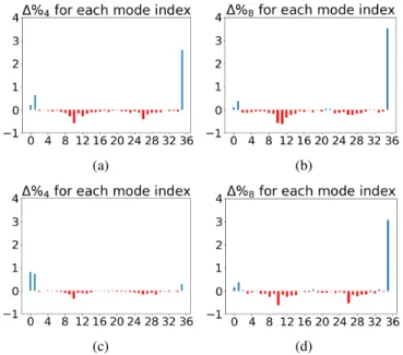
Fig. 14: Difference∆%w between the percentage of selection
an intra prediction mode in H.265-ITNN after the third training iteration and that after the first training iteration on the w×
w luminance blocks returned by the image partitioning: (a) w = 4 and QP = 22, (b) w = 8 and QP = 22, (c)w = 4
and QP = 27, (d) w = 8 and QP = 27. The index of the single additional neural network-based intra prediction mode is35. ∆%w is computed by averaging over the H.265-ITNN encodings of the124 YCbCr images used earlier.
H.265-ITNN should increase over iterations while those of the H.265 directional modes must decrease and those of PLANAR and DC should go up. This must be valid for small blocks at small QPs since the large blocks returned by the image partitioning at large QPs sometimes exhibit complex textures, see Section IV-B, and the behavior of a deep predictor on large blocks with diverse textures can hardly be forecast [9]. The previous assumption is verified by Figure 14. Therefore, for small blocks, the single additional mode takes a growing proportion of frequency of selection away from the H.265 directional modes over iterations and, as its signalling cost is much smaller [15], bitrates are saved.
VI. SIGNALLING OF THE NEURAL NETWORK-BASED INTRA PREDICTION MODE INH.266
Section V-A evaluates the rate-distortion performance of H.265 including the single additional neural network-based intra prediction mode. Before assessing the rate-distortion performance of H.266 with the single additional mode, a signalling of this mode in H.266 must be developed.
The first principle of the proposed signalling addresses the large number of neural networks in H.266 incurring a large memory cost. Indeed, blocks of each possible size are predicted by a different neural network belonging to the single additional mode, see Section III. As the H.266 partitioning can involve 25 different block sizes, the single additional mode in H.266 should be made of 25 neural networks. Note that the calculation of the previous figure excludes the option of splitting a luminance PB into multiple TBs because, as said
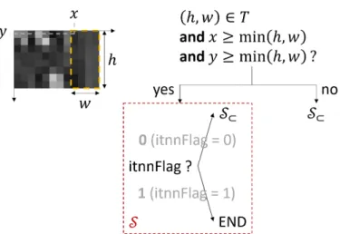
Fig. 15: Choice of the intra prediction mode signalling for the currentw×hluminance PB framed in orange. The first frame of “PartyScene” in 4:2:0 is being encoded via H.266-ITNN with QP= 37. The coordinates of the pixel at the top-left of this PB arex= 8andy= 0.h= 8andw= 4. The bin value of a itnnFlag value appears in bold gray.
in Section VI-A, the combination of the neural network intra prediction and this type of split is not allowed. This contrasts with the H.265 partitioning involving 5 different block sizes, the single additional mode thus comprising5neural networks only. As a deep neural network for intra prediction has a few million parameters, see Section V-A, the memory cost of the parameters of25neural networks in H.266 seems to be too high. To reduce this cost, only blocks of some sizes are predicted via neural networks. For each of these sizes, the pair of the height and width is inserted into the setT ⊆Q. Then, for the current block to be predicted, the single additional mode is signalled if it includes the neural network predicting blocks of the current block size.
Furthermore, the single additional mode should not be signalled when the neural network prediction cannot be carried out as the context of the current block to be predicted goes out of the image bounds.
A. Signalling for a luminance PB
Given the above-mentioned two principles, for a w ×h luminance PB whose top-left pixel is located at (x, y) in the image, the intra prediction mode signalling S including the flag itnnFlag of the single additional mode is chosen if (h, w) ∈ T and x ≥ min(h, w) and y ≥ min(h, w). Otherwise, another intra prediction mode signallingS⊂ which
does not compriseitnnFlag applies, see Figure 15.
Moreover, as the single additional mode yields predictions of good average quality over various luminance blocks, see Figures 8 to 13, according to entropy coding,itnnFlagshould be placed first inS, see Figure 15.itnnFlag= 1indicates that the single additional mode predicts the current luminance PB. Since VTM-5.0, H.266 has featured MIP, a machine learning-based intra prediction tool, see Section II-A. To compare in terms of rate-distortion H.266 to H.266 with the single additional mode, called H.266-ITNN, each codec having
a different machine learning-based intra prediction tool, MIP is removed from H.266-ITNN. Therefore,S⊂ denotes the H.266
intra prediction mode signalling for the current luminance PB without the MIP signalling. Note that, given Figure 15, the neural network-based intra prediction cannot be combined with Intra Sub-Partitions (ISP) [42], which allows to partition the current luminance PB into multiple TBs.
B. Signalling for a chrominance PB
As with luminance, the single additional mode gives predic-tions of good average quality over various chrominance blocks, implying that its signalling cost must be low for chrominance too. As the flag of the Direct Mode (DM) comes first in the intra prediction mode signalling for a chrominance PB in VTM-5.0 [43], we allow the neural network intra prediction of a chrominance PB via DM. Note that, since VTM-6.0, the DM flag has no longer been first in the intra prediction mode signalling for a chrominance PB since the Cross-Component Linear Model flag has been placed before it [44].
But, the use of the single additional mode via DM is restricted by the two principles laid down at the beginning of Section VI. To incorporate these constraints, for a given w×hchrominance PB whose top-left pixel is at(x, y)in the image, if the luminance PB collocated with this chrominance PB is predicted by the single additional mode, DM becomes the single additional mode if(h, w)∈T andx≥min(h, w)
andy≥min(h, w). Otherwise, DM is set to PLANAR.
C. Sizes of blocks predicted by the neural network-based mode Now, only the set T of pairs of the height and width of the blocks that can be predicted by the single additional mode remains to be defined. For non-square blocks, when the single additional mode includes neural networks predicting relatively small blocks, e.g. 4 × 8 blocks, and does not contain those predicting the large ones, e.g. 8×32 blocks, the rate-distortion performance is better compared to the other way round, see Section VII-B. By favoring the relatively small non-square blocks over the large ones, T = {(4,4),(4,8),(8,4),(8,8),(16,16),(4,16),(16,4),(8,16),
(16,8),(32,32),(64,64)}. Therefore, the single additional mode comprises11neural networks in H.266-ITNN.
VII. COMPARISON WITH THE STATE-OF-THE-ART
Now that the iterative training of neural networks for intra prediction is explained, see Section IV, and the single additional mode involving the trained neural networks can be integrated into both H.265 and H.266, see Section VI, the two codecs with the single additional mode, namely H.265-ITNN and H.266-ITNN, can be compared against the state-of-the-art. A. Comparison for H.265
In the literature on the enhancement of the H.265 intra prediction via neural networks, Progressive Spatial Recur-rent Neural Network (PS-RNN) [16], Intra Prediction Fully-Connected Networks (IPFCN) [11], the generative adversarial neural network-based intra prediction in [20], and the Neural Network-based intra prediction modes (NN-modes) [22], see Section II-B, stand out as the four benchmarked approaches.
TABLE III: BD-rate reductions in%of H.265-ITNN withl= 3, PS-RNN [16], IPFCN-D [11], and H.265 with the generative adversarial neural network-based intra prediction mode in [20]. As ITNN is built from HM-16.15, the anchor of H.265-ITNN is HM-16.15. For similar reasons, the anchors of PS-RNN, IPFCN-D, and H.265 with the generative adversarial neural network-based mode are HM-16.15, HM-16.9, and HM-16.17 respectively. Only the first frame of each video sequence is considered. All BD-rate reductions have one decimal digit, similarly to [11]. The largest BD-rate reduction in absolute value for the luminance channel is shown in bold. Note that, using the current experimental setups, HM-16.15 and HM-16.17 yield the same rate-distortion scores. Therefore, HM-16.15 and HM-16.17 are two equivalent anchors.
Video sequence our H.265-ITNN PS-RNN [16] IPFCN-D [11] Generative method [20]
Y Cb Cr Y Cb Cr Y Cb Cr Y Cb Cr B BasketballDrive −8.5 −9.7 −9.5 −1.4 −1.1 −1.4 −3.6 −2.9 −2.7 −0.9 0.2 −1.5 BQTerrace −4.1 −4.4 −4.0 −2.4 −0.5 −0.5 −2.1 −1.3 −0.5 −7.2 −8.6 −8.6 Cactus −4.2 −4.1 −4.2 −2.3 −1.5 −0.9 −3.2 −1.8 −1.5 −2.3 −2.2 −2.8 Kimono −3.2 −3.8 −2.9 −1.2 −0.9 −0.9 −3.1 −2.1 −1.5 −0.0 −0.7 −1.0 ParkScene −2.3 −4.0 −3.4 −2.7 −1.6 −1.3 −3.6 −2.2 −2.4 −1.0 −1.6 −1.0 C BasketballDrill −5.6 −7.9 −7.1 −1.6 −0.3 −1.5 −1.5 −3.3 −2.2 −11.1 −10.3 −11.6 BQMall −4.1 −5.0 −5.5 −3.0 −1.4 0.0 −2.2 −1.9 −1.0 −17.3 −18.6 −20.4 PartyScene −3.0 −3.0 −2.8 −2.5 −2.2 −2.2 −1.6 −1.2 −0.1 −7.9 −9.3 −9.4 RaceHorses −3.8 −4.1 −3.2 −2.3 −1.8 −1.0 −3.2 −1.9 −2.8 −0.8 −0.9 −1.7 D BasketballPass −3.8 −4.3 −4.1 −2.1 −1.9 −0.5 −1.2 −0.3 1.1 −0.1 0.6 0.6 BlowingBubbles −3.0 −5.2 −4.3 −2.7 −2.2 0.5 −1.9 −2.8 −3.5 −1.8 −5.3 −5.0 BQSquare −3.3 −2.0 −1.9 −2.1 −0.6 1.8 −0.9 −0.1 −2.8 −10.0 −12.3 −12.3 RaceHorses −5.3 −5.3 −6.3 −3.5 −3.3 −1.8 −3.2 −2.6 −2.8 −0.8 −1.3 −1.6 Mean −4.2 −4.8 −4.5 −2.3 −1.5 −0.7 −2.4 −1.9 −1.7 −4.7 −5.4 −5.9
1) Comparison with [16], [11], [20]: The experimental setup shared by [16], [11], [20] is reproduced. Specifically, only the first frame of each video sequence from the classes B, C, and D of the CTC [38] is considered. The rate-distortion performance of H.265 including a neural network-based intra prediction mode is calculated via the Bjontegaard metric of this modified version of H.265 with respect to H.265 with QP∈ {22,27,32,37}. All intra is used as configuration.
IPFCN comes in two variants, namely Intra Prediction Fully-Connected Networks Single (IPFCN-S) and Intra Pre-diction Fully-Connected Networks Dual (IPFCN-D), the latter featuring an enhanced training process. Indeed, in IPFCN-S, four fully-connected networks are designed to predict blocks of sizes4×4,8×8,16×16, and32×32respectively. Then, each neural network is trained on pairs of a luminance block returned by the H.265 partitioning of images and its context. Finally, the four trained neural networks are aggregated into a neural network-based mode in H.265. In contrast, in IPFCN-D, the above-mentioned set of fully-connected networks is duplicated into two sets. Then, the different pairs of a lumi-nance block given by the H.265 partitioning of images and its context are clustered into two groups, the first one gathering the blocks predicted via either PLANAR or DC and the second one containing those predicted via a directional mode. Each of the two sets of neural networks is trained on a different cluster. In the end, the two sets of trained neural networks form the neural network-based mode in H.265. As IPFCN-D outperforms S in terms of rate-distortion [11], IPFCN-D is picked for comparison.
Table III shows that, for the luminance channel, H.265-ITNN using three training iterations yields −1.8% of addi-tional mean BD-rate reduction compared to IPFCN-D. With respect to PS-RNN, the additional mean BD-rate reduction reaches −1.9%. The approach in [20] gives −0.5% of addi-tional mean BD-rate reduction with respect to H.265-ITNN. But, the complexity of the prediction mechanism in [20] far exceeds those of H.265-ITNN, PS-RNN, and IPFCN-D.
Indeed, in [20], for a givenw×wPB,w∈ {4,8,16,32,64}, a 17-layer convolutional neural network predicts the64×64
block whose top-left pixel matches the top-left pixel of the w×w PB, and the prediction of the w×w PB is obtained by cropping the w×w area at the top-left of the 64×64
neural network prediction. In contrast, in H.265-ITNN, PS-RNN, and IPFCN-D, a smaller neural network directly returns aw×wprediction of a givenw×wPB. This makes a sensitive difference in decoder run time, see Section VII-C.
2) Comparison with [22]: As several experimental setups in [22] differ from those shared by [16], [11], [20], another experiment following the experimental setups in [22] compares H.265-ITNN to NN-modes. This time, all the frames of each video sequence from the classes A, B, C, and D used in [22] are considered. As in Section VII-A1, QP∈ {22,27,32,37} and the configuration is all intra.
For the luminance channel, H.265-ITNN using three train-ing iterations yields −1.25% of additional mean BD-rate reduction with respect to NN-modes, see Table IV. Note that, as NN-modes refers to VTM-1.0 with multiple neural network-based intra prediction modes, its anchor is VTM-1.0. Although H.265-ITNN and NN-modes do not have the same anchor, their comparison is still valid in regard to intra prediction for two reasons. Firstly, only the partitioning changes from HM-16.15 to VTM-1.0. Indeed, VTM-1.0 amounts to HM-HM-16.15 with QuadTree plus Binary Tree and Ternary Tree [45], [46]. Secondly, given that each mode in NN-modes predicts blocks of each size via a different neural network, the performance of the neural network-based intra prediction should barely be affected by the modifications of partitioning.
B. Comparison for H.266
As H.266 includes MIP since VTM-5.0, the evaluation of H.266-ITNN, which is built from VTM-5.0 without MIP, with respect to VTM-5.0 establishes a direct comparison between our single additional mode and MIP. The experimental pro-tocol in this section takes the propro-tocol from Section VII-A1,
TABLE IV: BD-rate reductions in % of H.265-ITNN with l = 3 and NN-modes [22]. For H.265-ITNN, the anchor is H.265 (HM-16.15). For NN-modes, the anchor is VTM-1.0. All the frames of each video sequence are considered. All BD-rate reductions have two decimal digits, similarly to [22]. The largest BD-rate reduction in absolute value for the luminance channel is shown in bold.
Video sequence our H.265-ITNN NN-modes [22]
Y Cb Cr Y Cb Cr A Tango2 −6.81 −6.77 −9.42 −5.20 −4.31 −3.42 FoodMarket4 −13.42 −11.90 −12.35 −5.67 −2.90 −3.06 CampfireParty −2.63 −3.70 −3.74 −1.44 −0.88 −1.29 CatRobot1 −4.79 −5.37 −5.80 −3.66 −2.69 −1.96 DaylightRoad2 −4.52 −8.07 −8.16 −4.01 −1.60 −2.47 ParkRunning3 −2.49 −2.99 −2.95 −1.93 −1.81 −2.24 B MarketPlace −2.50 −3.75 −4.61 −3.11 −1.33 −0.48 RitualDance −5.35 −5.59 −7.24 −5.49 −2.89 −2.68 BasketballDrive −6.90 −8.89 −9.19 −2.92 −1.95 −2.00 BQTerrace −3.85 −4.76 −4.24 −2.60 −0.60 0.10 Cactus −4.09 −4.45 −4.37 −3.88 −2.17 −1.99 C BasketballDrill −6.13 −5.58 −5.89 −2.51 −2.32 −2.61 BQMall −4.32 −4.17 −5.52 −4.40 −2.47 −2.29 PartyScene −2.94 −3.19 −2.87 −2.89 −1.56 −1.62 RaceHorses −3.36 −4.33 −3.21 −2.78 −1.63 −1.88 D BasketballPass −4.12 −4.23 −3.90 −3.43 −2.22 −2.52 BlowingBubbles −3.13 −4.24 −4.14 −2.71 −1.63 −2.00 BQSquare −3.33 −3.59 −2.43 −2.84 −0.79 −1.05 RaceHorses −4.24 −5.12 −7.35 −3.74 −2.43 −2.00 Mean −4.68 −5.30 −5.65 −3.43 −2.01 −1.97
except that eight video sequences from the class A of the CTC are added in order to diversify the test data.
Due to the increase of encoder run time from HM to VTM, the commonly used deep neural networks for intra prediction cannot currently be trained in reasonable time via the proposed iterative training with H.266 as codec. Indeed, even though the encoder run time of H.265-ITNN is50times larger than that of HM-16.15, see section VII-C, the encoding ofΓvia H.265-ITNN does not exceed4days using400cores. However, as the ratio between the encoder run time of VTM-5.0 and that of HM-16.15 is nearly 18, the encoding of Γ
via H.266 with the single additional mode seems to be too long. Two solutions could be the optimization of the neural network architectures for faster inference [47], [48] and the implementation of heuristics for VTM encoder acceleration. But, these heuristics have not been developed yet since the H.266 standard is not finalized yet. For now, the models trained iteratively with H.265 as codec can be inserted into H.266 at test time. Therefore, the following experiments involve two versions of H.266-ITNN. For the “true” H.266-ITNN, blocks of sizes4×4,8×8,16×16, and32×32are predicted by the four neural networks trained iteratively with H.265 as codec and l = 3, the blocks of sizes 8×4,4×8, 16×4, 4×16,
16×8,8×16, and64×64being predicted by neural networks trained as in [15], c.f. Section II-B. For the second version, called H.266-STNN, any block whose pair of height and width belongs to T is predicted by a neural network trained as in [15]. STNN stands for Simply Trained Neural Networks.
H.266-ITNN gives −0.22% of additional mean BD-rate reduction with respect to H.266-STNN, see Table V. Thus, a noticeable improvement of the rate-distortion performance of H.266 with the single additional mode can be attributed to
TABLE V: BD-rate reductions in % of H.266-STNN and H.266-ITNN. The anchor is VTM-5.0. Only the first frame of each video sequence is considered. The largest BD-rate reduction in absolute value for the luminance channel is displayed in bold.
Video sequence H.266-STNN H.266-ITNN
Y Cb Cr Y Cb Cr A CampfireParty −1.16 −0.53 −0.30 −1.29 −0.61 −0.25 DaylightRoad2 −1.76 0.57 −2.32 −2.04 −1.00 −1.58 Drums2 −1.44 −1.64 −1.03 −1.63 −1.76 −1.10 Tango2 −2.54 −2.35 −1.96 −2.95 −2.09 −3.03 ToddlerFountain2 −1.45 −2.25 −1.00 −1.56 −2.07 −1.31 TrafficFlow −1.09 0.83 0.20 −1.45 1.57 0.58 PeopleOnStreet −2.68 −3.27 −2.88 −2.84 −2.90 −3.15 Traffic −1.87 −1.52 −1.30 −1.97 −1.62 −1.90 B BasketballDrive −1.84 −1.75 −2.15 −2.03 −1.34 −2.22 BQTerrace −1.58 −0.51 −0.65 −1.75 −0.22 −1.67 Cactus −1.76 −0.81 −1.48 −2.00 −1.38 −1.65 Kimono −1.38 −2.56 −1.94 −1.48 −2.72 −2.51 ParkScene −1.18 −1.65 −2.08 −1.22 −0.71 0.45 C BasketballDrill −1.06 0.65 −0.41 −1.26 0.50 −1.94 BQMall −2.21 −1.80 −1.89 −2.60 −1.14 −1.11 PartyScene −1.96 −3.16 −0.88 −2.15 −2.88 −1.32 RaceHorses −1.84 −0.34 −1.86 −1.90 −1.18 0.09 D BasketballPass −1.19 −3.41 −4.13 −1.73 −0.46 −3.02 BlowingBubbles −1.80 −0.64 −0.10 −2.05 −1.65 1.00 BQSquare −1.86 0.96 −2.54 −2.13 1.63 −2.98 RaceHorses −2.00 −3.67 −1.15 −2.27 −1.90 −1.88 Mean −1.70 −1.37 −1.52 −1.92 −1.14 −1.45
TABLE VI: mean BD-rate reduction per class in% of H.266-ITNN and VTM-5.0 with MIP on. The anchor is VTM-5.0 with MIP off. Only the first frame of each of the video sequences in Table V is considered. The largest mean BD-rate reduction in absolute value for the luminance channel is written in bold. “Mean” refers to an average over video sequences, not over classes.
Class Y H.266-ITNNC VTM-5.0 with MIP on
b Cr Y Cb Cr A -2.36 −1.35 −1.63 −0.37 −0.05 −0.16 B -2.03 −1.32 −1.18 −0.34 −0.05 0.33 C -2.26 −1.81 −1.83 −0.28 −0.65 −0.75 D -2.49 −1.23 −1.49 −0.41 −0.56 0.19 Mean -2.28 −1.41 −1.54 −0.35 −0.26 −0.09
the iterative training whereas only a relatively small fraction of the blocks are actually predicted by iteratively trained neural networks. By extending the iterative training to the 11
neural networks in H.266-ITNN, a much larger increase in mean BD-rate reduction can be expected. Moreover, Table V reports a mean BD-rate reduction of−1.92%for H.266-ITNN. This experimental result shows the advantage of the single additional deep neural network-based mode over the multiple MIP modes. A visualization of reconstruction via H.266-ITNN is displayed in Figure 16.
To assess the net benefit of the single additional mode to H.266, the anchor can now be set to VTM-5.0 with MIP off. The mean BD-rate reduction of H.266-ITNN becomes −2.28%, see Table VI.
Finally, to justify the choice of T for H.265-ITNN in Section VI-C, H.266-ITNN is compared to H.266-ITNN-large for which(4,8)and(8,4)are replaced by(8,32)and(32,8)
inT, see Table VII. The drop in mean DB-rate reduction is significant when the single additional mode neglects several
(a) (b) (c) (d)
Fig. 16: Comparison of (a) the 64×64block whose top-left pixel is at(64,64)in the luminance channel of “BasketballDrill”, (b) its reconstruction via VTM-5.0, (c) its reconstruction via H.266-ITNN, and (d) its partitioning via H.266-ITNN. QP= 27. In (d), the mapping from the color of the frame of the block to the intra prediction mode of the block is “orange” → either PLANAR or DC, “black” →directional mode, and “blue” →neural network-based mode. For the entire luminance channel, for VTM-5.0, rate =0.310bpp and PSNR = 39.503 dB. For H.266-ITNN, rate =0.305bpp and PSNR= 39.491 dB. TABLE VII: mean BD-rate reduction per class in%of
H.266-ITNN and H.266-H.266-ITNN-large. The anchor is VTM-5.0. Only the first frame of each of the video sequences in Table V is considered. The largest mean BD-rate reduction in absolute value for the luminance channel is written in bold. “Mean” refers to an average over video sequences, not over classes.
Class H.266-ITNN H.266-ITNN-large
Y Cb Cr Y Cb Cr A -1.97 −1.31 −1.47 −1.68 −0.76 −1.09 B -1.70 −1.27 −1.52 −1.39 −0.67 −1.27 C -1.98 −1.17 −1.07 −1.86 −0.87 −1.00 D -2.04 −0.60 −1.72 −1.75 −0.61 −1.69 Mean -1.92 −1.14 −1.45 −1.68 −0.78 −1.27
small blocks and predicts more large blocks. C. Complexity
Table VIII compares the average encoder run times and decoder run times of H.265-ITNN, PS-RNN [16], IPFCN-D [11], and the generative method in [20] on CPU only. A Intel Xeon CPU E5-2690 is used to compute the average run times of H.265-ITNN. The authors in [22] report that, when NN-modes is compared to VTM-1.0, the average encoder run time reaches 284% and the average decoder run time equals 147%. Therefore, the encoder and decoder slowdowns caused by the integration of the multiple neural network-based intra prediction modes in [22] into a HEVC-like codec are much smaller than those reported in [16], [11], [20], and in the approach in the current paper. This must arise from the relatively small neural network architectures used in [22]. Moreover, the average decoder run time of [20] reaches
526400%. Thus, the average decoder run time of the generative method in [20] exceeds those of H.265-ITNN, PS-RNN, and IPFCN-D by an order of magnitude. This must be explained by the complexity of the prediction mechanism in [20], see Section VII-A1.
The drop of encoder run time from H.265-ITNN to H.266-ITNN in Table VIII is due to the implementation. Indeed, in H.266-ITNN, as the neural network-based intra prediction cannot be coupled to ISP, see Section VI-A, the neural network
prediction of a given luminance PB tested by the encoder can be computed only once.
VIII. CONCLUSION
This paper has introduced an iterative training of neural networks for intra prediction in a block-based codec. At each iteration, the neural networks become more beneficial intra predictors for this codec as the training sets are filled with pairs of a block and its context typically found in the codec image partitioning and for which the neural network intra prediction can outdo the codec intra prediction. When inserted into both H.265 and H.266, the iteratively trained neural networks bring significant improvements in terms of rate-distortion.
REFERENCES
[1] Alasdair Newson, Andr´es Almansa, Matthieu Fradet, Yann Gousseau, and Patrick P´erez, “Video inpainting of complex scenes,”SIAM Journal on Imaging Sciences, vol. 7, no. 4, pp. 1993–2019, October 2014. [2] Zhaobin Zhang, Yue Li, Li Li, Zhu Li, and Shan Liu, “Multiple linear
regression for high efficiency video intra coding,” inICASSP, 2019. [3] Soochan Lee, Junsoo Ha, and Gunhee Kim, “Harmonizing maximum
likelihood with GANs for multimodal conditional generation,” inICLR, 2019.
[4] Haofeng Li, Guanbin Li, Liang Lin, and Yizhou Yu, “Context-aware semantic inpainting,” IEEE Transactions on Cybernetics, vol. 49, no. 12, pp. 4398–4411, October 2019.
[5] Ian Goodfellow, Jean Pouget-Abadie, Mehdi Mirza, Bing Xu, David Warde-Farley, Sheryl Ozair, Aaron Courville, and Yoshua Bengio, “Generative adversarial nets,” inNIPS, 2014.
[6] Jiahui Yu, Zhe Lin, Jimei Yang, Xiaohui Shen, Xin Lu, and Thomas S. Huang, “Generative image inpainting with contextual attention,” in
CVPR, 2018.
[7] Satoshi Iizuka, Edgar Simo-Serra, and Hiroshi Ishikawa, “Globally and locally consistent image completion,” ACM Transactions on Graphics, vol. 36, no. 4, pp. 1–14, July 2017.
[8] Yong-Goo Shin, Min-Cheol Sagong, Yoon-Jae Yeo, Seung-Wook Kim, and Sung-Jea Ko, “PEPSI++: fast and lightweight network for image inpainting,” arXiv:1905.09010v3, October 2019.
[9] Deepak Pathak, Philipp Kr¨ahenb¨uhl, Jeff Donahue, Trevor Darell, and Alexei A. Efros, “Context encoders: feature learning by inpainting,” in
CVPR, 2016.
[10] Tingzhu Sun, Weidong Fang, Wei Chen, Yanxin Yao, Fangming Bi, and Baolei Wu, “High-resolution image inpainting based on multi-scale neural network,”Electronics, vol. 8, no. 11, November 2019.

![TABLE III: BD-rate reductions in % of H.265-ITNN with l = 3, PS-RNN [16], IPFCN-D [11], and H.265 with the generative adversarial neural network-based intra prediction mode in [20]](https://thumb-us.123doks.com/thumbv2/123dok_us/8927671.2376274/12.918.79.841.212.432/table-reductions-ipfcn-generative-adversarial-neural-network-prediction.webp)
