Research Article
Broad Learning System with Locality Sensitive Discriminant
Analysis for Hyperspectral Image Classification
Huang Yao ,
1Yu Zhang,
1Yantao Wei ,
1,2and Yuan Tian
11School of Educational Information Technology, Central China Normal University, Wuhan 430079, China 2Educational Informatization Research Center of Hubei, Central China Normal University, Wuhan 430079, China Correspondence should be addressed to Yantao Wei; [email protected]
Received 12 August 2020; Revised 23 September 2020; Accepted 30 September 2020; Published 8 December 2020 Academic Editor: Jiayi Ma
Copyright © 2020 Huang Yao et al. This is an open access article distributed under the Creative Commons Attribution License, which permits unrestricted use, distribution, and reproduction in any medium, provided the original work is properly cited. In this paper, we propose a new method for hyperspectral images (HSI) classification, aiming to take advantage of both manifold learning-based feature extraction and neural networks by stacking layers applying locality sensitive discriminant analysis (LSDA) to broad learning system (BLS). BLS has been proven to be a successful model for various machine learning tasks due to its high feature representative capacity introduced by numerous randomly mapped features. However, it also produces redundancy, which is indiscriminate and finally lowers its performance and causes heavy computing demand, especially in cases of the input data bearing high dimensionality. In our work, a manifold learning method is integrated into the BLS by inserting two LSDA layers before the input layer and output layer separate, so the spectral-spatial HSI features are fully utilized to acquire the state-of-the-art classification accuracy. The extensive experiments have shown our method’s superiority.
1. Introduction
Hyperspectral images (HSIs) are produced by hyperspectral sensors by capturing reflectance values on tens or even hundreds of spectral bands for each pixel. The increased spectral resolution of HSIs makes them essential for many remote sensing tasks in various fields, such as agriculture [1], environment [2], and military [3], etc. To obtain semantic abstraction from HSIs, classification requires mapping from pixel values to land-use and/or land-cover descriptions, which is nontrivial because the high spectral redundancy detrimentally affects the classification process in terms of the curse of dimensionality problem [4] and noisy labels [5]. Moreover, accompanied by increasing spatial resolution, the widespread adoption of integrated spatial and spectral in-formation in HSIs’ analysis has further increased the di-mensionality of input data [6]. It has been proven in many cases that the useful spectral information for HSIs classifi-cation implies a nonlinear embedded submanifold of the original feature space, which can be retrieved by manifold-learning-based feature extraction methods [7, 8]. Sun et al. modified isometric mapping (ISOMAP) by accelerating its
process to reduce the dimensionality of HSIs [9]. Fauvel et al. investigated the kernel principal component analysis (KPCA) cooperating with a linear classifier in HSIs classi-fication and showed its privilege over the original principal component analysis method [10]. In contrast to previous global approaches, locally based methods like locally linear embedding (LLE) [11] and Laplacian eigenmaps (LE) [12] merely attempt to preserve the local geometrical structure of data, thus bringing about two prominent advantages: computational efficiency and representation capacity [13]. Some recent researches tried to formulate locally based manifold learning with a supervised regularization, thereby creating discriminative and compact feature representations [14–16]. Locality sensitive discriminant analysis (LSDA) [17] was developed as an extension to linear discriminant analysis (LDA) by integrating the discriminative properties of LDA with the nearest neighborhood graph (NNG) modeling the local geometrical structure of the underlying manifold. Unlike other NNG based approaches (e.g., locality preserving projections (LPP) [18] and LE) [12], LSDA was used within-class graph and between-class graph to obtain good between-class separation and preserve the within-class
Volume 2020, Article ID 8478016, 16 pages https://doi.org/10.1155/2020/8478016
local structure as well. It can then be expected as a useful feature reduction method for supervised classification tasks. During the past decades, machine learning methods have been widely used to achieve higher semantic prediction accuracy on HSIs. For example, kernel machines such as support vector machine (SVM) and kernel Fisher dis-criminant analysis (KFDA) have been used successfully for HSIs classification [19]. Ensemble learning methods like random forest [20] and rotation forest [21] also showcased their benefits, especially when the available labeled training samples are limited [22]. Inspired by the biological nervous system, neural network models have achieved great success in general media information processing [23] and HSIs analysis [24, 25]. Moreover, models with random weights (NNRW) such as random vector functional link networks (RVFL) [26], Schmidt’s method [27], and extreme learning machine (ELM) [28] set arbitrary weights and biases for the hidden layer while the weights for output layer are obtained analytically. As noniterative artificial neural network (ANN) based frameworks, the NNRW algorithms enable high training efficiency while still retaining the powerful repre-sentation learning capacity [29]. In the field of HSIs clas-sification, Xia et al. [30] reported that the general ELM was more accurate and much faster than SVM. Zhou et al. compared ELM with the composite kernel (ELM-CK) to SVM with CK (SVM-CK) and revealed that the ELM-based method still holds its advantages [31].
Recently, a new NNRW method, which broadly extends the hidden layer of RVFL called broad learning system, has been introduced [32, 33]. The main distinctive feature of BLS is that the input data are randomly mapped to features in “feature nodes,” which are subsequently transformed by nonlinear activation function to form “enhancement nodes.” Such a higher-order network structure provides an alter-native way of learning deep features. In addition, the uni-versal approximation capability of a broad learning system has been proven [33]. Jin et al. developed a robust broad learning system (RBLS) by modifying the regular terms of the cost function in order to promote its generalization performance on contaminated data modeling [34]. Through replacing the feature nodes with Takagi–Sugeno (TS) fuzzy subsystems, Feng and Chen crafted a neurofuzzy model called fuzzy broad learning system for regression and classification tasks [35]. Kong et al. applied BLS to HSIs classification for the first time. The semisupervised frame-work enabled the proposed method (i.e., semisupervised BLS (SBLS)) to leverage limited labeled samples and substantial unlabeled samples [36]. Although SBLS has shown its ad-vantages over many approaches, including deep learning-based methods, the potential of BLS in HSIs classification is far from being fully exploited under the current situation.
In this paper, we propose a new framework for HSIs classification called BLS-LSDA, which integrates hierar-chical spectral-spatial information abstraction, manifold learning method, and BLS. Our method firstly extracts spectral-spatial features by iteratively abstracting pixels’ neighborhood in a hierarchical manner. Then the features
are input into manifold learning nodes implementing LSDA. The reduced dimensional features, which are discriminative and locality preserving, are sent to the feature nodes and afterward, the enhancement nodes of BLS. The following layer which is identical to the previous LSDA one is adopted to exploit the intrinsic structure of high order features produced by random mapping. At last, the weights of output nodes are acquired by a ridge regression learning algorithm. Our contributions are highlighted as follows:
(1) Our method integrates a manifold learning algo-rithm with BLS in a multilayer neural network model, thus providing enhanced feature represen-tation capacity to BLS
(2) A novel implementation of spectral-spatial response (SSR) [37] consisting of Gabor filter and adaptive weighted filter (AWF) is developed to extract deep features of HSIs without a deep learning scheme (3) With comparative experiments conducted on 3
standard HSIs datasets, we show the proposed approach’s advantage in classification accuracy over the state-of-the-art methods
The rest of this paper is organized as follows. Section 2 gives a brief overview of BLS. In section 3, we present our method along with the details of the learning algorithm. Section 4 compares the performance of our method in three benchmark datasets with several prominent approaches and analyses the experimental results. Finally, discussions and conclusions are given in section 5.
2. Broad Learning System
Being different from the deep neural networks (DNN), BLS has no need of gradually searching for the models’ optimized parameters with backpropagation (BP).
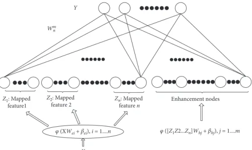
The learning procedure of BLS consists of only one step, e.g., performing matrix inversion to figure out the weights of links between the nodes of the hidden layer and output layer. As a single hidden layer feedforward neural network (SLFN), the most prominent characteristic of BLS is the adoption of mapped feature nodes to construct the enhancement nodes, which bring in higher feature representation capability. Figure 1 shows the framework of the original BLS. Given the input data setX, theithgroup of mapped feature nodes can be established by the following:
Zi�φi XWei+βei, (1)
where Wei is the randomly chosen weights, andβei is the
bias. It should be noted that different functions φi can be
adopted for the n different groups of the mapped nodes. Concatenating the mapped nodes, we get the following:
Zn �Z1, Z2,. . ., Zn. (2)
ThenZn is fed into the enhancement nodes to produce
Em�ϕ ZnWhm+βhm, (3)
whereWhmandβhmare weights and biases, respectively,φis
the activation function. Usually, sigmoid function is used. Eventually, the hidden layer of BLS is as follows:
H� φ1 XW1+β1,φ2 XW2+β2,. . .,φn XWn+βn|ϕ Z n Whm+βhm � Z1, Z2,. . ., Zn|ϕZ n Whm+βhm �ZnEm. (4)
Then the output layer can be obtained by the following:
Y�HWmn, (5)
where Wm
n is the connection weights between the BLS’s
hidden layer nodes and output layer nodes. Since theHand
Y are already known in the learning procedure, we can calculate Wm
n by rigid regression of the pseudoinverse as
follows:
Wmn �ZnEm+Y. (6)
3. Methods
3.1. MultiScale Composite Spatial Features. Spatial infor-mation has been utilized for hyperspectral image classifi-cation for many years [38, 39], along with the recognition that a smoother classification map always ensures higher classification accuracy [40]. However, for those pixels lying along the edges, a smoothing filter may jeopardize the classification accuracy gain. Thus, in most cases, the spatial information derived by smoothing filters was composed with the raw spectral band values to acquire a trade-off of the based and isolated pixel values [31], or
context-sensitive adaptive filters were designed to give out the edge-preserving maps [41]. In this work, we utilize the adoptive weighted filter (AWF) proposed by Zhou and Wei [42] to extract spatial information from HSIs. Meanwhile, given its deficiency in obtaining the differential information and inspired by the success of Gabor features applying in hyperspectral image analysis by enhancing the spatial dis-crimination on the highly contrastive area [43, 44], we exploit the benefit of integrating a simple two-dimensional Gabor filter and the AWF for feature extraction.
By assuming that neighborhood pixels which have similar spectrum distribution are more likely to belong to the same class, AWF obtains the weight of each pixel in the neighborhood by evaluating the similarity between it and the central pixel of the filter as follows:
wi,j� si,j
mi,j×msi,j. (7)
The similarity si,j is calculated by the Gaussian radial basis function as follows:
si,j�exp − pcentral−pi,j �� �� � ����� 2 σ ⎛ ⎜ ⎜ ⎝ ⎞⎟⎟⎠, (8)
wherepcentralis the central pixel andpi,jis the pixel located at theithrow andjthcolumn of the neighborhood. Theσis the standard deviation of the pixels’ difference, as follows:
σ�stdd1,1,. . ., d1,m, d2,1,. . ., dm,m, di,j������pcentral−pi,j�����.
(9)
Derived from the computational model for human be-ings’ visual cortical channels, the 2D Gabor filter (https://en. wikipedia.org/wiki/Gaborfilter) has been widely used in
Z1: Mapped
feature1
Y
Z2: Mapped
feature 2 Znfeature : Mapped n
Enhancement nodes
φ (XWei + βei), i = 1....n φ ([Z1Z2...Zn]Whj + βhj), j = 1....m
Wm
n
X
Figure1: In the BLS framework, the mapped features are adopted as the input of enhancement nodes and the output layer nodes, thus introducing better representation capacity.
computer vision for various low-level tasks [45, 46]. It is a directional sinusoidal function modulated by a Gaussian envelope on a 2D (h, v) plane, which can be expressed in the complex form as follows:
g(h, v;λ,θ,ψ,ω,c) �exp −h′ 2 +c2v′2 2ω2 ⎛ ⎝ ⎞⎠×exp i 2πx
′
λ+ψ , (10) where h′�hcosθ+vsinθ, v′� −hsinθ+vcosθ, (11)whereλdenotes the wavelength of the sinusoidal factor,θis the orthogonal orientation to the parallel stripes of a Gabor function.ψ is the phase offset,σ denotes the standard de-viation of the Gaussian envelope, andcis the spatial aspect ratio that specifies the ellipticity of the support of the Gabor kernel.
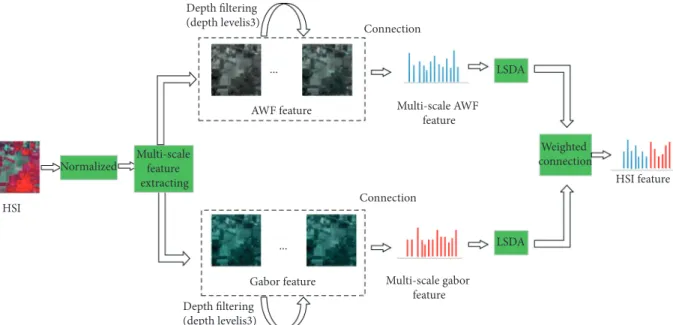
The two spatial features are then integrated into a multiscale framework. We extract AWF and Gabor features through 5×5, 7×7, 9×9, 11×11, and 13×13 filters, re-spectively. At each scale, the convolution is conducted 3 times iteratively, and then the obtained features are sent to the next step. Figure 2 shows a brief view of the extraction of the multiscale composite spatial features.
3.2. BLS-LSDA. We believe that the validity of BLS greatly roots from its numerous randomly constructed hidden nodes which form a “broad” neural network structure. However, excessive nodes generally cause heavy computa-tional or storage consumption, especially when the number of input nodes is boosted. Moreover, the randomly produced nodes have been often criticized for their arbitrariness that may deteriorate the performance in real-world applications [47].
The underlying structure of input data which is useful for classification can be retained by discriminate analysis methods, which intend to seek feature representations that address the interclass separation. It is necessary for BLS to make a compromise between the arbitrarily created nodes and their usefulness in differentiating input features of varied classes. To fulfill this task, an effective way is to in-troduce LSDA into BLS. Deriving from LDA, LSDA over-whelms its prototype by revealing the local geometrical structure of the data manifold additionally. In this work, we craft a novel neural network model named BLS-LSDA by inserting two layers applying LSDA as in Figure 3. Details of the layers are listed as follows.
(1) A layer was added between the input layer and the hidden layer of BLS to decrease the dimensionality of input data as well as enhance its separability; (2) By inserting an extra layer applying LSDA between
the hidden layer and output layer, we further
introduce a groupwise feature mapping which will benefit the weights retrieving.
For each LSDA layer, given m samples
x1, x2,. . ., xm
∈Rn, and their labels l(x1), l(x2),. . ., l(xm)
as input, LSDA splits the nearest neighbors ofxiintoNw(xi)andNb(xi)which are thexi’s nearest neighbor sample sets of the same and different labels, respectively.
Nw xi�xjil x ij�l xi,1≤j≤k, Nb xi�xjil x ij≠l(x),1≤j≤k,
(12)
where k denotes the number of nearest neighbors of xi. Based on Nw(xi) and Nb(xi), within-class graph Gw and
between-class graphGbare constructed with weight matrices
Ww andWb. Ww,ij� 1, ifxi∈Nw xiorxj∈Nw xi, 0, otherwise, Wb,ij� 1, ifxi∈Nb xiorxj ∈Nb xi. 0, otherwise. (13)
In order to map the points in feature space to a line so that the within-class points stay as close as possible while the between-class points stay as far as possible, given the map as
yT� (y
1, y2,· · ·, ym) �aTX, where X� (x1,· · ·, xm) is a n×mmatrix, the projection vector acan be retrieved by,
argmaxaa T X αLb+(1−α)WwX T asubject toaTXDwX T a�1, (14)
where Lb is the Laplacian matrix, Dw is a diagonal matrix withDw,ii�jWw,ij. Andαis a scalar between 0 and 1. See [17] for details.
Algorithm 1 depicts the framework of the BLS-LSDA training process. LetXgtrbe the Gabor andXftrbe the AWF features of sampleXtr. They are fed into the first LSDA layer separately to produce dimensional reduced featuresXgtr′ and Xftr′. Then the two features are weighted and concatenated as follows:
Xtrs �λXgtr′,(1−λ)Xftr′. (15)
According to equations (1) and (3), now we get the groups of feature nodes and enhancement nodes of BLS-LSDA as follows:
Zi�φ XstrWei+βei, Em�ϕ ZnWhm+βhm.
(16)
Each group of mapped features and enhancement fea-tures are fed into the second LSDA layer separately, and then we concatenated the outputs to get [Zn′|Em′] (see Algo-rithm 1). At last, the weights of the output layer are cal-culated with equation (6).
Y Enhancement Nodes Zn Z2 Zi = φ(XstrWei + βei), i = 1....n Xstr = [λXgtr′(1 – λ)Xftr′] Em = ϕ(ZnW hm + βhm) Z1 Zn′ Z2′ Z1′ Em E′ m LSDA LSDA Wm n Xgtr Xftr Xgtr′ Xftr′
Figure3: In the framework of BLS-LSDA, two layers applying LSDA are inserted into the original BLS network to increase the rep-resentation learning capability.
Normalized ... ... AWF feature Gabor feature LSDA LSDA Connection Connection Multi-scale AWF feature Multi-scale gabor feature HSI feature HSI Multi-scale feature extracting Weighted connection Depth filtering (depth levelis3) Depth filtering (depth levelis3)
Figure2: The overview of the extraction of the multiscale composite spatial features. The multiscale AWF and Gabor features are extracted and concatenated with chosen weights to form the final HSI features.
4. Experimental Result and Analysis
4.1. Datasets. To investigate the performance of our pro-posed framework, three open remote sensing datasets shown in Figure 4 have been taken as benchmarks. The first one is the Indian Pine dataset, which was collected by Airborne
Visible/Infrared Imaging Spectrometer (AVIRIS) sensor over the Indian Pines test site located in North-western Indiana, USA. The scene consisting of 145×145 pixels was captured with 224 spectral bands in the wavelength ranging 0.4–2.5×10⁻⁶meters. The number of labeled samples in its 16 classes is quite unbalanced, ranging from 20 to 2455. In
(a) (b)
Figure4: Three open hyperspectral imagery datasets used in our experiment. (a) From top to down are the raw imageries from the Indian Pine, the Pavia University, and the Salinas. (b) The corresponding ground-truth maps.
our experiment, only 200 bands were used in order to avoid the effect of water absorption.
The second dataset is the Pavia University dataset col-lected by the Reflective Optics System Imaging Spectrometer (ROSIS) sensor with 115 bands. The dataset has a spatial size of 610×340 pixels with 9 labeled land-cover classes. Due to the noise, 12 bands are discarded in our experiment.
Salinas dataset was also captured by AVIRIS sensor while being characterized by high spatial resolution (3.7 m/pixel). The ground-truth covered contains 16 classes. 20 water absorption bands were also removed from the Salinas in the experiment.
4.2. Parameter Settings. To quantitatively compare the classification results of BLS-LSDA with some prominent or state-of-the-art methods, including SVM, KELM, SVM-CK, KELM-CK [31], HiFi-We [48], and MASR [49], three fre-quently used indexes as overall accuracy (OA), average accuracy (AA), and kappa coefficient (K) are adopted in our experiment. For each time, class-wiser(r�5, 10, 15, 20, 25, 30, 35, 40) labeled samples randomly chosen from each dataset are used for training, while the left is taken as testing samples (When there are no sufficient labeled samples, half of them are selected for training). To make the comparison more reliable, each listed evaluation result is obtained by taking an average of 10 times measurements under the same model settings. Moreover, in order to show the main features of our method, some parameters are manually chosen, as shown in Table1. The analysis of parameters’ sensitivities can be found in section 4.4.
4.3. Classification Results. We present our experimental results on each dataset in Tables (2), (3), and (4). Based on the results shown in all tables, we can find that our proposed BLS-LSDA is superior to the classic methods (i.e., SVM and KELM) and their derivations with spectral-spatial kernel method (i.e., SVM-CK and KELM-CK), as well as recent prominent methods (i.e., HiFi-We and MASR) focusing on exploring the advantage of spectral-spatial filters in HSI classification. Moreover, in order to explore the utility of LSDA layers inserted into the BLS model, the classification results using the original BLS are also provided.
For the Indian Pines dataset, our method achieves up to 94.2±0.95% OA, 97.0±0.49% AA, and 93.3±1.10%k
when 40 training samples are used. The advantage of our method over classic methods is much more obvious than it over other methods; however, MASR is better than the proposed method on AA by nearly 0.3%. However, for the University of Pavia dataset, by using the same number of training samples, the classification accuracies
are 94.8±0.79% OA, 96.0±0.66% AA, and 93.0±1.09%
k, which surpass all the chosen comparative methods by 3-4% generally. For the Salinas dataset, our BLS-LSDA also achieved higher OA (98.0±0.43%), AA (99.1±0.18%), andk
(97.7±0.48%) than all other compared methods.
The advantage of BLS-LSDA is more obvious when there are a limited number of training samples (i.e., 5, 10, and 15). As an example, in Table (2), when 10 random samples are used for training, our method claims a nearly 4% OA in-crease over HiFi-We, which achieves the highest OA in comparative methods with 81.6±2.26%. We believe that it is due to the high representation learning capacity of our proposed network structure. Moreover, the classification accuracies’ standard deviations of our method are overall lower than other methods, which means that the proposed model is more robust to the randomly chosen training data. However, an exception to the previous statement can be found in Table 3, indicating that when there are extremely limited training samples, LSDA may fail to capture the representative features.
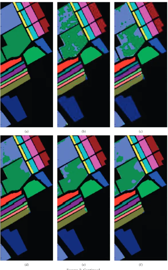
Figures 5, 6, and 7 visually show the classification results of BLS-LSDA and other compared methods whenr�40. By visual evaluation, we can conclude that our proposed method is good at balancing the classification accuracy of pixels at both sharp and smooth regions. Taking the Salinas dataset (Figure 7) as an example, it can be easily seen that our method surpasses the other methods on the homogeneous area (i.e., the two smooth patches marked with grey circles), while the edges or acute angles are also well-preserved.
4.4. Parameters’ Sensitivities Analysis. We have evaluated the impact of different values of the model’s parameters shown in Table 1. It reveals that the classification results are not sensitive to differenth,C,ands. Also, sinceN1,N2, and
N3 are intertwining, we choose these parameters empiri-cally. Besides, it has been well recognized that the di-mensionality of the reduced subspace is crucial in manifold learning. Here, we investigate the performance of BLS-LSDA with different subspace dimensions on three benchmark datasets. For each dataset and each class, 20 training samples were randomly selected and the remaining samples were used for testing. All experiments were per-formed 10 times in order to get the average results. Figure 8 depicts the relationship between the classification results (OA) and the dimensions of the reduced subspace on three datasets.
For Indian Pines, we can find that when the dimensions of reduced subspace are less than 15, the overall accuracy goes up with the increase of the dimensions; otherwise, the curve becomes flat. Similar curves can also be observed
Table2: Results of classification accuracy (%) under different numbers of labeled training samples per class of the Indian Pines dataset
r Index SVM KELM SVM-CK KELM-CK HiFi-We MASR BLS BLS-LSDA
5 OA 44.6±3.94 48.1±4.09 59.0±3.17 65.5±4.42 72.2±4.12 66.7±4.14 72.0±3.17 75.4 ± 3.22 AA 59.4±2.41 60.5±2.73 71.9±3.83 78.6±2.30 83.0±2.67 80.9±1.86 82.7±1.77 84.0 ± 2.03 k 38.5±4.04 42.0±4.31 54.2±3.57 61.4±4.57 68.7±4.52 60.2±5.07 66.6±3.92 70.8 ± 3.97 10 OA 53.9±4.31 57.7±1.73 70.2±4.55 79.2±2.76 81.6±2.26 80.2±2.66 83.7±2.41 85.6 ± 1.61 AA 67.2±2.72 68.9±1.17 82.3±2.48 88.1±1.65 89.7±0.89 89.5±1.14 90.7±1.23 91.7 ± 0.79 k 48.5±4.69 52.5±1.93 66.6±4.99 76.5±3.08 79.2±2.49 76.9±3.18 81.0±2.86 83.2 ± 1.92 15 OA 59.6±2.80 60.6±2.12 77.4±1.96 83.2±1.59 86.0±3.06 84.6±1.62 85.2±1.48 88.0 ± 2.21 AA 71.5±1.63 72.9±0.90 86.9±1.41 91.2±0.86 92.6±1.36 91.6±0.83 92.0±0.90 93.2 ± 1.12 k 54.7±3.03 55.9±2.26 74.6±2.19 81.1±1.77 84.2±3.39 82.0±1.89 82.8±1.74 86.0 ± 2.59 20 OA 61.8±2.60 64.1±1.70 82.1±2.32 87.6±0.91 87.7±1.43 88.5±1.93 88.9±1.48 90.1 ± 2.06 AA 73.0±1.86 75.5±1.39 90.0±0.87 93.7±0.69 93.6±0.77 94.2 ± 0.89 93.6±0.96 94.0±1.37 k 57.1±2.82 59.7±1.87 79.7±2.55 85.9±1.03 80.0±1.61 86.7±2.26 87.1±1.74 88.6 ± 2.42 25 OA 64.4±1.75 67.5±1.71 84.4±1.55 89.4±1.50 89.7±2.32 90.5±1.01 89.9±2.13 91.7 ± 1.86 AA 75.8±1.25 77.7±0.87 91.4±0.89 94.6±0.78 94.9±0.79 95.3±0.47 94.5±0.84 95.5 ± 0.89 k 60.1±1.92 63.4±1.81 81.5±1.63 88.0±1.70 88.3±2.57 89.0±1.17 88.3±2.50 90.4 ± 2.17 30 OA 66.9±1.51 69.3±1.30 85.6±1.45 91.3±1.62 92.0±0.97 91.8±1.45 90.5±2.22 93.3 ± 1.22 AA 78.2±1.34 79.5±0.82 92.6±0.74 95.7±0.73 95.9±0.57 96.0±0.59 94.9±1.26 96.4 ± 0.45 k 62.9±1.47 65.8±1.64 83.7±1.64 90.0±1.83 90.9±1.09 90.5±1.68 89.0±2.61 92.2 ± 1.41 35 OA 68.7±2.16 71.7±1.52 86.6±1.08 91.6±1.57 92.6±1.15 93.0±0.78 91.0±1.04 93.5 ± 1.04 AA 78.6±1.90 80.9±0.91 93.1±0.89 96.1±0.76 95.9±1.66 96.2±0.28 95.3±0.40 96.5 ± 0.72 k 64.8±2.35 68.1±1.71 84.8±1.21 90.4±1.78 91.5±1.30 91.9±0.91 89.6±1.22 92.5 ± 1.21 (i) Require: Training samplesXtr, and the corresponding labelsYtr; the group of mapped nodes in BLSn.
(ii) Ensure: The weights of the output layer,Wm n.
(1) Extract the Gabor featureXgtrand AWF featureX f
tr of sampleXtr;
(2) FeedXgtr andX f
trinto the layer which implement LSDA, to produce dimensional reduced featuresX g′
tr andX
f′
tr; (3) Concatenate weightedXgtr′ andXftr′ by equation (15), yieldingXs
tr; (4) fori�1;i<n;i++ do
(5) Assign a random value toWeiandβei;
(6) Calculate the mapped feature valuesZi�φ(Xs
trWei+βei).
(7) end for
(8) Concatenate the mapped feature values to get a mapped feature groupZn� [Z
1, Z2,. . ., Zn];
(9) AssignWhm andβhmwith random values;
(10) Calculate the enhancement nodes withEm�ϕ(ZnWhm+βhm);
(11) Apply LSDA to eachZiinZnandEm in another LSDA layer to getZ n
′andEm′;
(12) ConcatenateZn′andEm′to produce[Z n
′|Em′];
(13) Calculate the connection weights between the BLS’s hidden layer and an output layer withWm n � [Z
n|E m]
+
Y.
ALGORITHM1: BLS-LSDA training algorithm.
Table1: Parameter settings of the proposed method for each dataset.
Dataset parameter Indian pines Pavia University Salinas
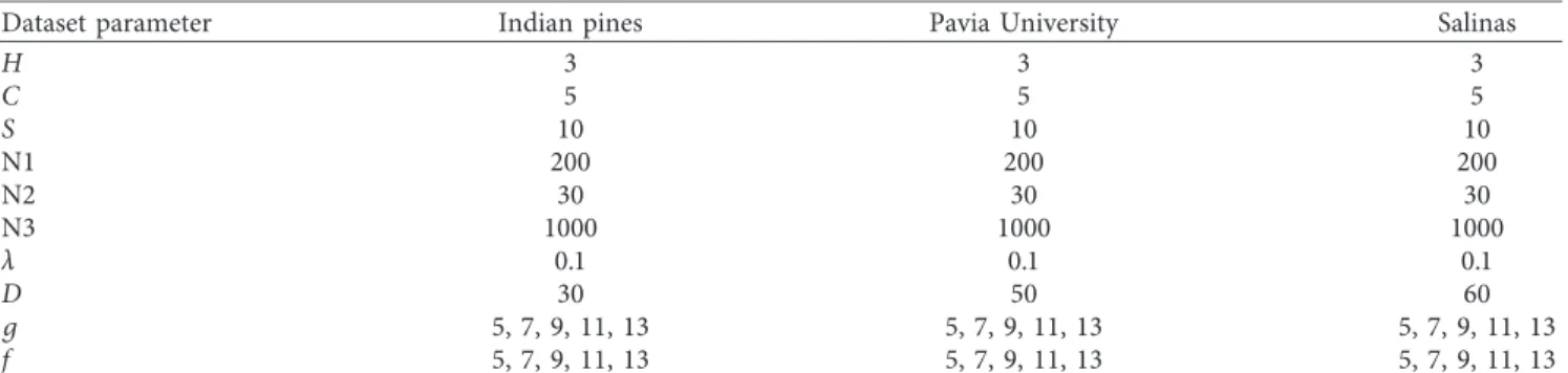
H 3 3 3 C 5 5 5 S 10 10 10 N1 200 200 200 N2 30 30 30 N3 1000 1000 1000 λ 0.1 0.1 0.1 D 30 50 60 g 5, 7, 9, 11, 13 5, 7, 9, 11, 13 5, 7, 9, 11, 13 f 5, 7, 9, 11, 13 5, 7, 9, 11, 13 5, 7, 9, 11, 13
his the convolution depth of Gabor and AWF filters,gandfare the neighborhood’s sizes of Gabor and AWF, respectively,λis the weight of the spatial information in equation (15),dis the number of dimensions of reduced subspace in LSDA algorithm,Candsare penalty parameters and enhanced node scaling in BLS, and N1, N2, and N3 are the number of feature node groups, feature nodes per group, and enhanced nodes in BLS, respectively.
Table2: Continued.
r Index SVM KELM SVM-CK KELM-CK HiFi-We MASR BLS BLS-LSDA
40
OA 70.1±1.48 72.1±1.98 89.1±1.28 93.4±0.87 93.1±1.10 94.0±0.66 91.7±1.11 94.2 ± 0.95 AA 81.2±3.46 81.1±1.27 94.4±0.66 96.9±0.35 96.3±0.57 97.3 ± 0.29 95.8±0.48 97.0±0.49 k 66.3±1.63 68.5±2.21 87.6±1.46 92.5±0.98 92.1±1.24 93.1±0.77 90.3±1.29 93.3 ± 1.10
Table3: Results of classification accuracy (%) under different numbers of labeled training samples per class of the University of Pavia dataset.
r Index SVM KELM SVM-CK KELM-CK HiFi-We MASR BLS BLS-LSDA
5 OA 57.8±6.36 58.8±4.44 65.3±8.89 64.1±7.98 66.3±6.54 69.0±2.19 74.2 ± 4.75 73.7±6.44 AA 70.6±2.42 67.9±2.30 73.5±3.55 71.6±3.38 73.1±2.13 70.5±1.81 81.9 ± 1.78 78.3±2.64 k 48.6±6.24 49.5±3.85 56.9±9.95 55.3±8.66 57.4±7.22 51.7±4.00 62.8 ± 6.73 60.8±9.90 10 OA 62.3±6.60 63.6±3.45 75.3±6.74 76.5±6.62 79.2±4.52 74.6±3.46 83.8±3.27 84.0 ± 2.81 AA 73.3±1.89 74.5±1.29 81.3±2.30 81.2±3.96 84.3±2.65 74.7±2.19 87.0±1.18 87.5 ± 1.75 k 53.8±6.55 55.0±3.49 70.0±6.70 70.3±7.87 73.6±5.28 61.4±6.00 77.2±4.59 77.4 ± 4.10 15 OA 69.6±4.09 67.1±3.99 82.7±4.52 83.9±4.56 83.2±2.58 79.0±2.89 86.2±2.31 88.4 ± 1.76 AA 76.8±1.32 77.4±1.09 85.3±2.08 86.4±1.98 86.7±1.97 79.3±1.09 90.2±1.27 90.7 ± 0.96 k 61.6±4.49 59.2±4.18 77.8±5.39 79.3±5.43 78.4±3.18 69.2±4.45 80.7±3.35 83.9 ± 2.48 20 OA 71.6±3.99 69.1±5.08 86.6±2.65 87.8±4.38 86.3±2.72 82.3±2.33 87.1±2.84 88.8 ± 1.91 AA 79.8±0.84 78.7±1.26 88.3±1.31 88.9±1.91 89.2±1.82 81.3±1.42 91.0±0.90 91.1 ± 0.80 k 64.3±4.30 61.5±5.36 82.6±3.26 84.2±5.39 82.2±3.33 74.4±3.55 82.1±3.93 84.6 ± 2.69 25 OA 72.3±4.29 73.4±2.30 88.4±2.36 88.8±3.27 87.0±2.43 85.6±1.78 88.3±2.27 89.7 ± 1.38 AA 80.2±2.07 80.8±0.92 89.7±1.49 90.3±1.34 90.3±1.90 84.1±0.56 91.8±0.83 92.2 ± 0.54 k 65.1±4.77 66.3±2.39 82.6±3.26 85.5±4.05 83.2±3.03 79.6±2.57 83.9±3.20 85.7 ± 1.93 30 OA 75.5±2.43 75.6±1.42 90.6±1.52 91.4±1.84 88.0±1.27 86.8±2.11 88.8±2.38 91.5 ± 1.44 AA 81.6±1.30 81.3±1.02 91.3±0.86 91.6±1.01 91.8±0.77 85.5±0.75 92.2±0.82 93.3 ± 0.85 k 68.7±2.79 68.9±1.61 87.7±1.93 88.7±2.35 84.5±1.57 81.3±3.06 84.5±3.31 88.3 ± 2.01 35 OA 76.9±3.34 75.7±2.09 91.2±1.26 91.9±1.52 88.3±3.12 88.1±1.43 88.9±2.67 93.2 ± 0.83 AA 82.5±1.29 82.3±0.91 91.8±0.89 92.5±0.97 91.9±1.28 86.9±0.74 92.3±1.20 95.1 ± 0.31 k 70.6±3.73 69.1±2.40 88.6±1.64 89.3±1.97 84.9±3.85 83.3±2.06 84.6±3.72 90.8 ± 1.13 40 OA 77.7±2.69 76.2±2.62 91.6±1.80 93.2±1.09 90.4±1.91 89.5±1.41 90.0±2.25 94.4 ± 0.85 AA 83.3±1.18 83.2±0.80 92.2±0.87 93.1±0.99 92.7±1.09 88.2±0.77 93.0±0.76 95.4 ± 0.52 k 71.4±3.21 69.8±2.97 89.0±2.27 91.1±1.43 87.4±2.43 85.4±1.99 86.3±3.14 92.3 ± 1.16 (a) (b) (c) Figure5: Continued.
(a) (b) (c) (d)
Figure6: Continued.
(d) (e) (f )
(g) (h) (i)
Figure5: Classification results on the Indian Pines dataset with 40 training samples per class. (a) The Ground-truth map. (b) SVM. (c) KELM. (d) SVM-CK. (e) KELM-CK. (f ) HiFi-We. (g) MASR. (h) BLS. (i) BLS-LSDA.
when the other two datasets are taken. However, the turning points are found when the number of dimensions equals 10.
We also investigate the change of classification accu-racies with λ. Figure 9 shows that with λ�0.1 the model acquires its best performance.
(e) (f ) (g) (h)
(i)
Figure6: Classification results on the University of Pavia dataset with 40 training samples per class. (a) The Ground-truth map. (b) SVM. (c) KELM. (d) SVM-CK. (e) KELM-CK. (f ) HiFi-We. (g) MASR. (h) BLS. (i) BLS-LSDA.
(a) (b) (c)
(d) (e) (f )
(g) (h) (i)
Figure7: Classification results on the Salinas dataset with 40 training samples per class. (a) The Ground-truth map. (b) SVM. (c) KELM. (d) SVM-CK. (e) KELM-CK. (f ) HiFi-We. (g) MASR. (h) BLS. (i) BLS-LSDA.
10 15 20 25 30 35 40 45 50 55 60 65 70 5
The dimensionality of the reduced subspace 30 40 50 60 70 80 90 100 O veral l acc urac y (%) Indian pines University of pavia Salinas
Figure 8: OA (%) of classification on 3 datasets with different dimensionality of reduced subspace.
Indian pines University of pavia Salinas 0.2 0.3 0.4 0.5 0.6 0.7 0.8 0.9 0.1 λ 70 75 80 85 90 95 100 O veral l acc urac y (%)
5. Conclusion
In this paper, we present a novel method for HSI classifi-cation which is based on BLS and LSDA. The two algorithms are integrated into a multilayered neural network model. To utilized both the spatial and spectral information, the Gabor filter and AWF filter are adopted to produce the input of the BLS-LSDA. Our experiments on three open benchmark datasets have shown their advantages against compared methods in terms of OA, AA, andk.
Also, our work has shown that with limited dimensional features acquired by LSDA layers in the model, high clas-sification accuracy can be achieved, which means compu-tational efficiency in real applications.
We believe that BLS-LSDA is a successful improvement on the original BLS for HSI classification; however, there are still some problems to be tackled. Our future work would address the initialization of weights and offsets with heuristic algorithms instead of random assignments.
Data Availability
The data used to support the findings of this study are available from the corresponding author upon request.
Conflicts of Interest
The authors declare that they have no conflicts of interest.
Acknowledgments
This work has been financially supported by the Funda-mental Research Funds for the Central Universities under Grant nos. CCNU20ZN002 and CCNU20TD005.
References
[1] F. A. Rodrigues, G. Blasch, P. BlasDefournych et al., “Multi-temporal and spectral analysis of high-resolution hyperspectral airborne imagery for precision agriculture: assessment of wheat grain yield and grain protein content,” Remote Sensing, vol. 10, no. 6, p. 930, 2018.
[2] D. Stratoulias, H. Balzter, A. Zlinszky, and V. R. T´oth, “A comparison of airborne hyperspectral-based classifications of emergent wetland vegetation at Lake Balaton, Hungary,” International Journal of Remote Sensing, vol. 39, no. 17, pp. 5689–5715, 2018.
[3] O. O. Fadiran and P. Moln´ar, “Maximizing diversity in synthesized hyperspectral images,” in Proceedings of the Targets and Backgrounds XII: Characterization and Repre-sentation, vol. 6239, October 2006, Article ID 623903. [4] W. Li and Q. Du, “A survey on representation-based
clas-sification and detection in hyperspectral remote sensing imagery,”Pattern Recognition Letters, vol. 83, pp. 115–123, 2016.
[5] J. Jiang, J. Ma, Z. Wang, C. Chen, and X. Liu, “Hyperspectral image classification in the presence of noisy labels,” IEEE Transactions on Geoscience and Remote Sensing, vol. 57, no. 2, pp. 851–865, 2019.
Table4: Results of classification accuracy (%) under different numbers of labeled training samples per class of the Salinas dataset.
r Index SVM KELM SVM-CK KELM-CK HiFi-we MASR BLS BLS-LSDA
5 OA 81.4±2.81 83.5±2.29 84.5±1.97 87.1±3.81 86.9±2.36 87.4±2.38 88.1±2.69 91.2 ± 1.22 AA 88.9±1.21 89.7±1.21 90.0±1.05 92.5±2.30 92.5±1.45 93.3±0.89 93.8±1.16 95.0 ± 0.69 k 79.3±3.05 81.7±2.50 82.8±2.16 85.7±4.22 85.4±2.59 86.0±2.62 86.7±3.00 90.2 ± 1.38 10 OA 85.6±1.13 86.5±1.73 88.3±1.08 89.6±2.91 88.9±1.17 90.9±1.48 92.8±1.76 94.3 ± 0.51 AA 91.6±0.77 92.3±1.06 92.7±1.04 94.8±0.97 94.3±0.46 95.8±0.64 96.6±0.94 97.2 ± 0.25 k 84.0±1.24 85.0±1.91 87.0±1.20 88.5±3.18 87.7±1.28 89.8±1.66 91.9±1.98 93.6 ± 0.57 15 OA 86.1±1.65 86.5±0.88 89.6±2.02 92.3±2.29 90.5±0.94 90.4±1.16 93.7±0.87 95.0 ± 0.91 AA 92.4±0.73 93.1±0.57 94.0±0.95 96.3±1.27 95.0±0.53 96.1±0.60 97.0±0.46 97.8 ± 0.42 k 84.6±1.82 85.0±0.98 88.5±2.23 91.4±2.54 89.5±1.05 89.3±1.30 93.0±0.98 94.4 ± 1.02 20 OA 87.0±1.18 88.1±0.59 92.0±0.85 93.9±0.92 90.8±1.01 93.3±1.24 93.9±1.06 96.4 ± 0.45 AA 93.2±0.60 93.9±0.58 95.8±0.42 97.3±0.49 95.3±0.46 97.1±0.61 97.4±0.39 98.3 ± 0.36 k 85.6±1.29 86.8±0.66 91.2±0.94 93.2±1.01 89.7±1.11 92.5±1.39 93.2±1.18 96.0 ± 0.51 25 OA 88.2±0.86 88.3±1.04 93.0±0.94 94.1±1.53 92.2±0.88 93.9±1.13 94.5±1.04 96.7 ± 0.68 AA 93.6±0.40 94.3±0.33 96.4±0.68 97.2±0.69 96.1±0.38 97.6±0.34 97.7±0.33 98.6 ± 0.25 k 86.9±0.94 87.0±1.14 92.2±1.04 93.4±1.70 91.3±0.97 93.2±1.26 93.9±1.16 96.4 ± 0.75 30 OA 88.2±1.02 88.5±0.56 93.1±1.70 95.0±1.22 92.4±0.97 94.2±1.19 94.7±0.89 97.1 ± 0.88 AA 93.9±0.76 94.5±0.29 96.4±0.67 97.9±0.42 96.3±0.33 97.6±0.38 97.7±0.31 98.8 ± 0.29 k 86.9±1.13 87.2±0.61 92.3±1.88 94.4±1.35 91.5±1.08 93.5±1.32 94.1±0.99 96.8 ± 0.98 35 OA 88.4±1.25 88.7±0.85 93.4±1.23 95.5±0.97 92.7±1.06 94.7±0.92 95.0±0.72 97.4 ± 0.39 AA 94.2±0.66 94.6±0.65 96.8±0.53 98.1±0.35 96.4±0.50 97.9±0.30 97.9±0.30 98.9 ± 0.14 k 87.1±1.37 87.5±0.95 92.6±1.37 95.0±1.07 91.8±1.18 94.1±1.03 94.5±0.81 97.1 ± 0.43 40 OA 89.1±1.10 88.9±0.99 93.7±1.46 96.3±0.39 92.9±0.54 95.9±0.50 95.2±0.64 98.0 ± 0.43 AA 94.6±0.36 94.9±0.42 97.0±0.92 98.3±0.13 96.4±0.23 98.3±0.21 97.9±0.28 99.1 ± 0.18 k 87.9±1.22 87.6±1.10 92.9±1.63 95.9±0.43 92.1±0.60 95.4±0.56 94.7±0.72 97.7 ± 0.48
[6] P. Ghamisi, E. Maggiori, S. Li et al., “New frontiers in spectral-spatial hyperspectral image classification: the latest advances based on mathematical morphology, markov random fields, segmentation, sparse representation, and deep learning,” IEEE Geoscience and Remote Sensing Magazine, vol. 6, no. 3, pp. 10–43, 2018.
[7] D. Lunga, S. Prasad, M. M. Crawford, and O. Ersoy, “Man-ifold-learning-based feature extraction for classification of hyperspectral data: a review of advances in manifold learn-ing,” IEEE Signal Processing Magazine, vol. 31, no. 1, pp. 55–66, 2014.
[8] J. Jiang, J. Ma, C. Chen et al., “SuperPCA: a superpixelwise PCA approach for unsupervised feature extraction of hyperspectral imagery,”IEEE Transactions on Geoscience and Remote Sensing, vol. 56, no. 8, pp. 4581–4593, 2018. [9] W. Sun, A. Halevy, J. J. Benedetto et al., “UL-Isomap based
nonlinear dimensionality reduction for hyperspectral imagery classification,”ISPRS Journal of Photogrammetry and Remote Sensing, vol. 89, pp. 25–36, 2014.
[10] M. Fauvel, J. Chanussot, and J. A. Benediktsson, “Kernel principal component analysis for the classification of hyperspectral remote sensing data over urban areas,”Eurasip Journal on Advances in Signal Processing, vol. 2009, Article ID 783194, 2009.
[11] S. T. Roweis and L. K. Saul, “Nonlinear dimensionality re-duction by locally linear embedding,” Science, vol. 290, no. 5500, pp. 2323–2326, 2000.
[12] M. Belkin and P. Niyogi, “Laplacian eigenmaps for dimen-sionality reduction and data representation,” Neural Com-putation, vol. 15, no. 6, pp. 1373–1396, 2003.
[13] V. D. Silva, V. De Silva, and J. B. Tenenbaum, “Global versus local methods in nonlinear dimensionality reduction,” Ad-vances in Neural Information Processing Systems, vol. 15, pp. 705–712, 2003, http://citeseerx.ist.psu.edu/viewdoc/ summary?doi�10.1.1.9.3407.
[14] X. Zhen, M. Yu, A. Islam, M. Bhaduri, I. Chan, and S. Li, “Descriptor learning via supervised manifold regularization for multioutput regression,” IEEE Transactions on Neural Networks and Learning Systems, vol. 28, no. 9, pp. 2035–2047, 2017.
[15] H. Yu, L. Gao, W. Li, Q. Du, and B. Zhang, “Locality sensitive discriminant analysis for group sparse representation-based hyperspectral imagery classification,” IEEE Geoscience and Remote Sensing Letters, vol. 14, no. 8, pp. 1358–1362, 2017. [16] P. Zhang, H. He, and L. Gao, “A nonlinear and explicit
framework of supervised manifold-feature extraction for hyperspectral image classification,”Neurocomputing, vol. 337, pp. 315–324, 2019.
[17] D. Cai, X. He, K. Zhou, J. Han, and H. Bao, “Locality sensitive discriminant analysis,” inProceedings of the 20th International Joint Conference on Artificial Intelligence, Ser. IJCAI’07, pp. 708–713, Morgan Kaufmann Publishers Inc., San Fran-cisco, CA, USA, January 2007.
[18] X. He and P. Niyogi, “Locality preserving projections,” in Proceedings of the 16th International Conference on Neural Information Processing Systems, Ser. NIPS’03, pp. 153–160, MIT Press, Cambridge, MA, USA, December 2003. [19] M. Chen, Q. Wang, and X. Li, “Discriminant analysis with
graph learning for hyperspectral image classification,”Remote Sensing, vol. 10, no. 6, p. 836, 2018.
[20] J. Xia, P. Ghamisi, N. Yokoya, and A. Iwasaki, “Random forest ensembles and extended multiextinction profiles for hyper-spectral image classification,” IEEE Transactions on Geo-science and Remote Sensing, vol. 56, no. 1, pp. 202–216, 2018.
[21] J. Xia, N. Falco, J. A. Benediktsson, P. Du, and J. Chanussot, “Hyperspectral image classification with rotation random forest via KPCA,”IEEE Journal of Selected Topics in Applied Earth Observations and Remote Sensing, vol. 10, no. 4, pp. 1601–1609, 2017.
[22] F. Li, L. Xu, P. Siva, A. Wong, and D. A. Clausi, “Hyper-spectral image classification with limited labeled training samples using enhanced ensemble learning and conditional random fields,” IEEE Journal of Selected Topics in Applied Earth Observations and Remote Sensing, vol. 8, no. 6, pp. 2427–2438, 2015.
[23] P. Yi, Z. Wang, K. Jiang, Z. Shao, and J. Ma, “Multi-temporal ultra dense memory network for video super-resolution,” IEEE Transactions on Circuits and Systems for Video Tech-nology, vol. 30, no. 8, pp. 2503–2516, 2020.
[24] H. Sun, X. Zheng, X. Lu, and S. Wu, “Spectral–spatial at-tention network for hyperspectral image classification,”IEEE Transactions on Geoscience and Remote Sensing, vol. 58, pp. 3232–3245, 2020.
[25] E. Pan, X. Mei, Q. Wang, Y. Ma, and J. Ma, “Spectral-spatial classification for hyperspectral image based on a single GRU,” Neurocomputing, vol. 387, pp. 150–160, 2020.
[26] Y.-H. Pao and Y. Takefuji, “Functional-link net computing: theory, system architecture, and functionalities,”Computer, vol. 25, no. 5, pp. 76–79, 1992.
[27] W. F. Schmidt, M. A. Kraaijveld, and R. P. Duin, “Feed forward neural networks with random weights,”vol. 2, pp. 1–4, inProceedings of the International Conference on Pattern Recognition, vol. 2, pp. 1–4, Institute of Electrical and Electronics Engineers Inc., Piscataway, NJ, USA, September 1992.
[28] G. B. Huang, Q. Y. Zhu, and C. K. Siew, “Extreme learning machine: a new learning scheme of feedforward neural net-works,” inProceedings of the IEEE International Conference on Neural Networks-Conference Proceedings, vol. 2, pp. 985–990, Los Alamitos, CA, USA, July 2004.
[29] W. Cao, X. Wang, Z. Ming, and J. Gao, “A review on neural networks with random weights,”Neurocomputing, vol. 275, pp. 278–287, 2018.
[30] J. Xia, N. Yokoya, and A. Iwasaki, “Classification of large-sized hyperspectral imagery using fast machine learning algo-rithms,” Journal of Applied Remote Sensing, vol. 11, no. 3, Article ID 035005, 2017.
[31] Y. Zhou, J. Peng, and C. L. Chen, “Extreme learning machine with composite kernels for hyperspectral image classifica-tion,”IEEE Journal of Selected Topics in Applied Earth Ob-servations and Remote Sensing, vol. 8, no. 6, pp. 2351–2360, 2015.
[32] C. L. Chen and Z. Liu, “Broad learning system: an effective and efficient incremental learning system without the need for deep architecture,”IEEE Transactions on Neural Networks and Learning Systems, vol. 29, no. 1, pp. 10–24, 2018.
[33] C. L. Chen, Z. Liu, and S. Feng, “Universal approximation capability of broad learning system and its structural varia-tions,”IEEE Transactions on Neural Networks and Learning Systems, vol. 30, no. 4, pp. 1191–1204, 4 2019.
[34] J. Jin, C. L. Chen, and Y. Li, “Robust broad learning system for uncertain data modeling,”vol. 1, pp. 3524–3529, in Pro-ceedings of the 2018 IEEE International Conference on Systems, Man, and Cybernetics, vol. 1, pp. 3524–3529, Institute of Electrical and Electronics Engineers Inc., Miyazaki, Japan, October 2018.
[35] S. Feng and C. L. Chen, “Fuzzy broad learning system: a novel neuro-fuzzy model for regression and classification,” IEEE Transactions on Cybernetics, vol. 50, pp. 414–424, 8 2018. [36] Y. Kong, X. Wang, Y. Cheng, and C. Chen, “Hyperspectral
imagery classification based on semi-supervised broad learning system,”Remote Sensing, vol. 10, no. 5, p. 685, 2018. [37] Y. Wei, Y. Zhou, and H. Li, “Spectral-spatial response for hyperspectral image classification,” Remote Sensing, vol. 9, no. 3, p. 203, 2017.
[38] Q. Jackson and D. A. Landgrebe, “Adaptive Bayesian con-textual classification based on Markov random fields,”IEEE Transactions on Geoscience and Remote Sensing, vol. 40, no. 11, pp. 2454–2463, 2002.
[39] S. Velasco-Forero and V. Manian, “Improving hyperspectral image classification using spatial preprocessing,”IEEE Geo-science and Remote Sensing Letters, vol. 6, no. 2, pp. 297–301, 2009.
[40] X. Cao, T. Xiong, and L. Jiao, “Supervised band selection using local spatial information for hyperspectral image,” IEEE Geoscience and Remote Sensing Letters, vol. 13, no. 3, pp. 329–333, 2016.
[41] X. Kang, S. Li, and J. A. Benediktsson, “Spectral-spatial hyperspectral image classification with edge-preserving fil-tering,”IEEE Transactions on Geoscience and Remote Sensing, vol. 52, no. 5, pp. 2666–2677, 2014.
[42] Y. Zhou and Y. Wei, “Learning hierarchical spectral-spatial features for hyperspectral image classification,”IEEE Trans-actions on Cybernetics, vol. 46, no. 7, pp. 1667–1678, 2016. [43] S. Jia, L. Shen, and Q. Li, “Gabor feature-based collaborative
representation for hyperspectral imagery classification,”IEEE Transactions on Geoscience and Remote Sensing, vol. 53, no. 2, pp. 1118–1129, 2015.
[44] W. Li and Q. Du, “Gabor-filtering-based nearest regularized subspace for hyperspectral image classification,”IEEE Journal of Selected Topics in Applied Earth Observations and Remote Sensing, vol. 7, no. 4, pp. 1012–1022, 2014.
[45] A. K. Jain and F. Farrokhnia, “Unsupervised texture seg-mentation using Gabor filters,”Pattern Recognition, vol. 24, no. 12, pp. 1167–1186, 1991.
[46] R. Mehrotra, K. R. Namuduri, and N. Ranganathan, “Gabor filter-based edge detection,” Pattern Recognition, vol. 25, no. 12, pp. 1479–1494, 1992.
[47] Y. Zhang, J. Wu, Z. Cai, B. Du, and P. S. Yu, “An unsupervised parameter learning model for RVFL neural network,”Neural Networks, vol. 112, pp. 85–97, 2019.
[48] B. Pan, Z. Shi, and X. Xu, “Hierarchical guidance filtering-based ensemble classification for hyperspectral images,”IEEE Transactions on Geoscience and Remote Sensing, vol. 55, no. 7, pp. 4177–4189, 2017.
[49] L. Fang, S. Li, X. Kang, and J. A. Benediktsson, “Spec-tral–spatial hyperspectral image classification via multiscale adaptive sparse representation,”IEEE Transactions on Geo-science and Remote Sensing, vol. 52, no. 12, pp. 7738–7749, 2014.