of peer-reviewed research and commentary in the population sciences published by the Max Planck Institute for Demographic Research Doberaner Strasse 114 · D-18057 Rostock · GERMANY www.demographic-research.org
DEMOGRAPHIC RESEARCH
VOLUME 7, ARTICLE 1, PAGES 1-14
PUBLISHED 02 JULY 2002
www.demographic-research.org/Volumes/Vol7/1/
DOI: 10.4054/DemRes.2002.7.1
Research Article
Decomposing demographic change
into direct vs. compositional components
James W. Vaupel
Vladimir Canudas Romo
1 Introduction 2 2 Formula for Decomposing Derivatives of Averages 2
3 Derivatives of Averages over Age 4
4 Death, Birth, Growth and Other Rates 7
5 Averages over Subpopulations 8
6 Other Decompositions 10
7 Acknowledgements 11
Notes 12
Research Article
Decomposing demographic change
into direct vs. compositional components
James W. Vaupel1
Vladimir Canudas Romo2
Abstract
We present and prove a formula for decomposing change in a population average into two components. One component captures the effect of direct change in the characteristic of interest, and the other captures the effect of compositional change. The decomposition is applied to time derivatives of averages over age and over subpopulations. Examples include decomposition of the change over time in the average age at childbearing and in the general fertility rate for China, Denmark and Mexico. A decomposition of the change over time in the crude death rate in Denmark, Germany and the Netherlands is also presented. Other examples concern global life expectancy and the growth rate of the population of the world.
1Director of Division 1 - Research Program on ”Aging” and Head of the Laboratory of Survival and
Longevity, Max Planck Institute for Demographic Research, Rostock, Germany
2Sergio Camposortega Cruz Ph.D. Fellow at the Max Planck Institute for Demographic Research, Rostock,
1. Introduction
Change in a population average can be accounted for in three alternative ways, which might be called level-0, level-1 and level-2 explanations. A level-0 explanation is simply that the data are erroneous. A level-1 explanation is that the observed population change is produced by a direct change in the characteristic of interest. A level-2 explanation is that the change is attributable to a change in the structure or composition of the population.
This article focuses on level-1 vs. level-2 explanations. We present a new method for decomposing change in a population average into two components, one capturing the ef-fect of direct change and the other capturing the efef-fect of compositional change. We begin with some notation and the proof of the decomposition formula. Then we provide some illustrative examples. In the examples shown here, two kind of compositional change are studied: change in the age-structure of the population and in the size of subpopulations.
2. Formula for Decomposing Derivatives of
Averages
Our results pertain to derivatives of averages, i.e., to change over instants of continuous time or some other continuous variable. The focus is on means, also known as expected values or expectations. LetE(v), the expectation operator, denote the mean value of
v(x;y)overx. This average will sometimes be denoted by the alternative notationv(y), with
E(v)E w
(v)v(y) = R
1 0
v(x;y)w(x;y)dx R
1 0
w(x;y)dx
; xcontinuous; (1)
= P
x v
x (y)w
x (y) P
x w
x (y)
; xdiscrete; (2)
wherev(x;y)is some demographic function andw(x;y)is some weighting function. The variablexcan be continuous or discrete; the variableyis continuous. In the applications presented in this article,xsometimes denotes age and sometimes subpopulations whereas
yis always time, but other application are also of interest.
We use a dot over a variable to denote the derivative with respect toy,
_
vv(x;_ y)= @ @y
and an acute accent to denote the relative derivative or intensity with respect toy,
vv(x; y)= @ @y v(x;y) v(x;y) = @ @y
ln[v(x;y)]: (4)
This use of the acute accent, which reduces the clutter in many demographic formulas, was originated by Vaupel (1992) and is used in Vaupel and Canudas Romo (2000). Note that for simplicity we often omit the argumentsxandy.
The key formula in this article was developed a decade ago by Vaupel (1992), who extended a result published by Preston, Himes and Eggers (1989). The formula can be simply and memorably expressed as
_ v=
_
v+Cov(v;w): (5)
The change in the average, _ v, is
_ v= @ @y R 1 0
v(x;y)w(x;y)dx R
1 0
w(x;y)dx
: (6)
The average change, _ v, is
_ v= R 1 0 h @ @y v(x;y) i w(x;y)dx R 1 0 w(x;y)dx : (7)
And the covariance can be calculated as
Cov(v;w) =E
(v;v) ; w; w
=E(vw) ;E(v)E(w)
= R
1 0
v(x;y)w(x; y)w(x;y)dx R 1 0 w(x;y)dx ; R 1 0
v(x;y)w(x;y)dx R 1 0 w(x;y)dx R 1 0
w(x;y)w(x;y)dx R 1 0 w(x;y)dx : (8) Proof
Ifv(x;y)andw(x;y)are continuous functions inxandy, then taking the derivative with respect toyin formula (1) yields
_ v= @ @y R 1 0
v(x;y)w(x;y)dx R
1 0
= R 1 0 h @ @y v(x;y) i
w(x;y)dx+ R 1 0 v(x;y) h @ @y w(x;y) i dx R 1 0 w(x;y)dx ; R 1 0
v(x;y)w(x;y)dx R 1 0 h @ @y w(x;y) i dx ;R 1 0 w(x;y)dx 2 = _ v+ R 1 0
v(x;y)w(x; y)w(x;y)dx R 1 0 w(x;y)dx ; R 1 0
v(x;y)w(x;y)dx R 1 0 w(x;y)dx R 1 0
w(x;y)w(x;y)dx R 1 0 w(x;y)dx = _
v+Cov(v;w):
A similar proof holds for the case whenv(x;y)andw(x;y)are discrete functions ofx. Q.E.D.
The first term on the right-hand side of (5), the average change, might be called the direct component of change; it captures the level-1 effect. The second component, the covariance term, is the structural or compositional component of change; it accounts for the level-2 effect of change in population heterogeneity. In formula (5) the covariance is a measure of the extent to which the underlying variable of interest rises and falls with the relative derivative of the weighting function.
3. Derivatives of Averages over Age
In several examples given here the weighting function,w(x;y), equalsN(a;t), the age-specific population size over ageaand timet. (See Arthur and Vaupel (1984) and Keiding (1990) for a discussion of this basic but subtle quantity.) For instance, by substituting age
aforv(x;y), the average age of a population can be calculated as
a=
R ! 0
aN(a;t)da R
! 0
N(a;t)da
; (9)
To study population aging, Preston, Himes and Eggers (1989) analyzed the derivative of formula (9). Following Ansley Coale’s suggestion that they consider the covariance, they found
_
a=Cov(a;r); (10)
wherer r(a;t)is the age-specific growth rate of the population. Becauser(a;t)
N(a;t)and becausea_ =0, formula (10) is a special case of (5) where there is no level-1 change. Schoen and Kim (1992) also derived a formula, similar to (10), in which there is only compositional change and no direct change.
Variants of (10) can be developed by letting the weighting function be given by
K(a;t) = k(a;t)N(a;t). If the functionk(a;t) = I(a), where I(a) is an indicator that equals zero ifa<65and one ifa65, then we have a formula for the average age of the elderly,
a 65 (t)= R ! 0 aK(a;t)da R ! 0 K(a;t)da = R ! 65 aN(a;t)da R ! 65
N(a;t)da
: (11)
The change in the average age of the elderly is given by
_ a 65 =Cov K (a; K); (12)
where the subscriptKsignifies that the weighting function in the covariance isK(a;t). The indicator does not depend on time, so
I =0. The relative derivative ofK(a;t)can therefore be simplified to
K=
@ @t
[I(a)N(a;t)] I(a)N(a;t)
= I+ N=
N; (13)
yielding _ a 65 =Cov K
(a;r); (14)
where, as before,r(a;t)is the age-specific growth rater(a;t) N(a;t).
To study the dynamics of average age at, say, childbearing,k(a;t)would beb(a;t), the age-specific birth rate among women at timet. ThenK(a;t)=b(a;t)N
f
(a;t), where N
f
(a;t)denotes the age-specific size of the population of women. In this caseK(a;t)is equivalent toB(a;t), the number of babies born to women of ageaat timet. Lettinga
_ a B =Cov B (a; b+r
f
); (15)
wherer f
(a;t) is the age-specific growth rate of the population of women,r f
(a;t)
N f
(a;t).
The covariance has the property that
Cov(v;w 1
+w 2
)=Cov(v;w 1
)+Cov(v;w 2
): (16)
Hence formula (15) can be expressed as
_ a B =Cov B (a; b)+Cov
B (a;r
f
): (17)
Note there is no “direct” effect in the way discussed earlier. Instead there are two “compo-sitional” effects. The effects describe the extent to which change in average age at child-bearing is due to change in age-specific births rates vs. change in the age composition of the population. For scholars interested in how age-specific birth rates affect average age at childbearing, the first termCov
B (a;
b)could be considered as capturing the change in the variable of interest whereas the second termCov
B (a;r
f
)would measure compositional change of the female population.
Table 1 shows the decomposition of the change in the average age at childbearing,
a B
(t), for China, Denmark and Mexico. The formula fora B
(t)is continuous but
de-Table 1: Average age at childbearing,a B
(t), and the decomposition of the annual
change over time from 1990 to 1995 for China, Denmark and Mexico.
China Denmark Mexico
a B
(1990) 25.352 28.231 26.784
a B
(1995) 25.147 29.254 27.234
_ a B
(1992:5) -0.041 0.205 0.090
Cov B
(a;
b) -0.131 0.172 0.039
Cov B
(a;r f
) 0.091 0.033 0.051
_ a B =Cov B (a; b )+Cov
B (a;r
f
) -0.040 0.205 0.090
Source: Authors’ calculations described in the Note, based on U.S. Census Bureau (2001).
mographic data are discrete, so we estimated the values in the table using the methods described in the Note at the end of this article. In China the average age at childbearing fell despite the aging of the female population. The change in age-specific birth rates cap-tured by theCov
B (a;
The last row of Table 1 shows the change in the average age at childbearing as the sum of the decomposition terms, _
a B
=Cov B
(a; b)+Cov
B (a;r
f
):These values are;0:040 for China, 0:205 for Denmark and 0:090 for Mexico. The estimated value for China is slightly different from the actual figure of;0:041. This discrepancy arises because discrete data over a 5-year period are used to approximate derivatives and averages at an instant (see Note). Similar small discrepancies can be found in other tables in this article.
4. Death, Birth, Growth and Other Rates
Let the functionv(x;y)be equivalent to the force of mortality(a;t)at ageaand timet and let the weighting function be the age-specific population size. Then it follows directly from formula (5) that
_ =
_
+Cov(;r); (18)
where(t) is the crude death rate of the population, sometimes denoted byd(t). Table 2 illustrates formula (18), by determining the decomposition of the change in the crude death rate for Denmark, Germany and the Netherlands from 1991 to 1997.
Table 2: Crude death rate,d(t), per thousand, and the decomposition of the annual
change over time from 1991 to 1997 for Denmark, Germany and the Netherlands.
Denmark Germany Netherlands
d(1991) 11.562 11.397 8.627
d(1997) 11.341 10.495 8.701
_
d (1994) -0.037 -0.150 0.012
_
-0.074 -0.273 -0.075
Cov(;r) 0.037 0.124 0.087
_ d=
_
+Cov(;r) -0.037 -0.149 0.012
Source: Authors’ calculations described in the Note, based on EUROSTAT (2000).
Germany benefited from sizeable reductions in the crude death rate in the years after reunification. On the other hand, its neighbors Denmark and the Netherlands experienced only small changes during this period. The German development is mainly due to the direct effect of large reductions in mortality, particularly in the eastern part of Germany. Note that in Germany both the level-1 and level-2 effects are larger than in Denmark and the Netherlands.
Similarly, letb(a;t)denote the age-specific birth rate, letN f
number of babies divided by the number of women at reproductive ages. The change in this rate is given by
_ g=
_
b+Cov(b;r f
): (19)
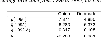
Table 3 shows calculations based on formula (19) that decompose the change in the GFR for China, Denmark and Mexico from 1990 to 1995. Table 3 indicates that the GFR fell in
Table 3: General fertility rate,g(t), in percentage, and the decomposition of the
annual change over time from 1990 to 1995, for China, Denmark and Mexico.
China Denmark Mexico
g(1990) 7.871 4.850 11.083
g(1995) 6.283 5.373 9.671 _
g(1992:5) -0.317 0.105 -0.282
_
b -0.280 0.081 -0.286
Cov(b;r f
) -0.036 0.023 0.004
_ g=
_
b+Cov(b;r f
) -0.316 0.104 -0.282
Source: Authors’ calculations described in the Note, based on U.S. Census Bureau (2001).
China and Mexico and rose in Denmark. In all three countries the dominant component of this shift was the average change in age-specific birth rates. Changes in age-composition, captured by the covariance term, had a relatively minor impact, especially in Mexico.
More generally, v(x;y)could be identified with some age-specific migration rate, morbidity rate, criminality rate, etc., and a formula similar to (18) and (19) would follow. An interesting case is whenv(x;y)is equivalent to the age-specific growth rate. Then
_ r=
_
r+Cov(r;r)=
_ r+
2
(r); (20)
so the change in a population’s growth rate is given by the average change in the age-specific growth rates plus the variance in the age-age-specific growth rates.
5. Averages over Subpopulations
Consider a population composed of different subpopulations. The life expectancy at birth at timetfor the entire population,e
o
(t), is the average over the subpopulations’ life expectancy at birth
e o (t)= P i e o;i (t)N i (t) P i N i (t) ; (21) whereN i
(t)is the size of subpopulationiande o;i
(t)is the subpopulation life expectancy at birth. The change ineover time can be decomposed as
_ e o = _ e o +Cov(e o
;r); (22)
wherer i
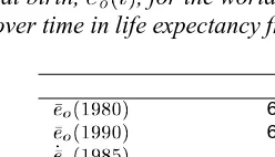
(t)is the population growth rate of theith subpopulation,r i (t) N i (t). In Table 4 formula (22) is applied to changes in life expectancy of the world popula-tion. The world experienced an increase in life expectancy with an annual change of more
Table 4: Life expectancy at birth,e o
(t), for the world and decomposition of the
annual change over time in life expectancy from 1980 to 1990.
World e o (1980) 62.790 e o (1990) 65.401 _ eo(1985) 0.261 _ eo 0.314 Cov(eo;r) -0.053 _ e o = _ e o +Cov(e o ;r) 0.261
Source: Authors’ calculations described in the Note, based on World Bank data (2001). The subpopulations are
the populations of the countries of the world for which data were available.
than three months per year (_ e o
(1985)=0:26). The covariance between life expectancy and population growth rates among the subpopulations is modest. Hence the change in the world life expectancy is roughly the same as the average change in life expectancy of the world’s countries. Because the covariance is negative, the countries with long life expectancy tend to have slow rates of population growth. The increase in life expectancy of the world is thus lower than the average increase in national life expectancy.
by the average change in growth rates of the countries plus the variance in the growth rates
_ r=
_ r+
2 (r):
Two theoretical implications deserve note. First, if the population growth rate of every country were constant (albeit at different levels from country to country), then the popu-lation growth rate of the world would be increasing. The countries with the largest growth rates would account for a larger share of the world’s population. Second, even if the pop-ulation growth rate of every country were declining, the world’s poppop-ulation growth rate could be increasing.
Table 5: Population growth rate of the world,r(t) , and decomposition of the annual
change over time around January 1, 1979 and around January 1, 1982.
t 1979 1982
r(t;1:5) 1.722 % 1.732 %
r(t+1:5) 1.732 % 1.711 %
_
r(t) 0.328
-0.716
_
r -0.459
-1.545
2
(r) 0.787
0.829
_ r=
_ r+
2
(r) 0.328
-0.716
Source: Authors’ calculations described in the Note, based on U.S. Census Bureau (2001). Note:
denotes per 10,000. Growth rates were calculated over intervals of 5 years (1975-1980, 1978-1983, 1981-1986) to estimate growth rates for 1977.5, 1980.5 and 1983.5. Growth rates were estimated based on data for all the countries of the world for which data were available.
As shown in Table 5, the population growth of the world started to decline around 1980. The pace of this decline was slowed by the variance in growth rates among the world’s countries. The average change in country growth rates,
_
r, was negative but the variance term more than offset this in the late 1970s, yielding an increase in the rate of world population growth of 0.328 per 10,000.
6. Other Decompositions
In the examples above, the weighting function was associated with either age-specific population size or national population size. Many other kinds of subpopulations could be considered. The subpopulations might reflect social, ethnic, religious, socio-economic or other characteristics. Suppose, for instance, a population consists of a number of subpop-ulations with different crude birth ratesb
i
(t)and different growth ratesr i
the birth rate of the overall population. Then the decomposition of the change over time in the birth rate is
_ b=
_
b+Cov(b;r): (23)
Alternatively, w(x;y)could be taken as representing the composition of the stable population implied by a population’s age-specific birth and death rates or the composition of the lifetable population implied by a population’s age-specific death rates. In the latter case, w(x;y)would be equal to `(a;t), which, defined with radix one, is simply the lifetable probability of surviving from birth to ageain periodt.
In addition, various demographic quantities can be substituted for the functionv(x;y). Formula (5) provides a simple but powerful approach for decomposing direct vs. com-positional change in many applications. In this article we provide a few illustrative ex-amples. Many other applications are possible. Such applications will help demographers understand the dynamics of population change.
7. Acknowledgments
Notes
If data are available for timeyandy+h, then we generally used the following approxi-mations for the value at the mid-pointy+h=2. For the relative derivative of the function
v(x;y+h=2),
v(x;y+h=2) ln
h
v( x;y+h) v(x;y)
i
h
: (24)
The value of the function at the mid-pointv(x;y+h=2)was estimated by
v(x;y+h=2)v(x;y)e
(h=2)v(x;y+h=2)
: (25)
Substituting the right-hand side of (24) forv(x; y +h=2)in (25) yields the equivalent approximation
v(x;y+h=2)[v(x;y)v(x;y+h)] 1=2
: (26)
This is a standard approximation in demography (Preston, Heuveline and Guillot, 2001). The derivative of the functionv(x;y+h=2)was estimated by
_
v(x;y+h=2)=v(x; y+h=2)v(x;y+h=2): (27)
We used (24)-(27) wherever we thought that the rate of change was more or less constant over the time interval. In a couple of cases it seemed appropriate to assume that change in the interval was linear. This was the case for estimating the change in the age-specific death rates in Table 2 and the change in the population growth rate in Table 5. Then we used
v(x;y+h=2)
v(x;y+h)+v(x;y) 2
(28)
and
_
v(x;y+h=2)
v(x;y+h);v(x;y) h
References
Arthur, W. Brian and James W. Vaupel. (1984). “Some general relationships in population dynamics.” Population Index, Summer, 50(2): 214-26.
Eurostat, New Cronos CD-ROM 2000. http://europa.eu.int/comm/eurostat/.
Keiding, Niels. (1990). “Statistical Inference in the Lexis Diagram.” Philosophical Trans-actions of the Royal Society of London 332: 487-509.
Preston, Samuel H., Patrick Heuveline and Michel Guillot. (2001). Demography:
Mea-suring and Modeling Population Processes. Oxford: Blackwell Publishers.
Preston, Samuel H., Christine Himes, and Mitchell Eggers. (1989). “Demographic Con-ditions Responsible for Population Aging.” Demography, November, 26(4): 691-703.
Schoen, Robert and Young J. Kim. (1992). “Covariances, roots, and the dynamics of age-specific growth.” Population Index, Spring 58(1): 4-17.
U.S. Census Bureau. Washington, D.C. (15/3/2001). http://www.census.gov/.
Vaupel, James W. and Vladimir Canudas Romo. (2000). How Mortality Improvement Increases Population Growth. In: Dockner E.J., Hartl R.F., Luptacik M., Sorger G.
Op-timization, Dynamics and Economic Analysis: Essays in Honor of Gustav Feichtinger.
Vienna: Springer: 350-57. Available at http://www.demogr.mpg.de/Papers/Working/wp-1999-015.pdf.
Vaupel, James W. (1992). “Analysis of Population Changes and Differences: Methods for Demographers, Statisticians, Biologists, Epidemiologists, and Reliability Engineers.” Paper (107 pp.) presented at the PAA Annual Meeting held in Denver, Colorado, April 30 - May 2 1992.