University of New Orleans University of New Orleans
ScholarWorks@UNO
ScholarWorks@UNO
University of New Orleans Theses and
Dissertations Dissertations and Theses
5-14-2010
Hull Shape Optimization for Wave Resistance Using Panel Method
Hull Shape Optimization for Wave Resistance Using Panel Method
Krishna M. Karri
University of New Orleans
Follow this and additional works at: https://scholarworks.uno.edu/td
Recommended Citation Recommended Citation
Karri, Krishna M., "Hull Shape Optimization for Wave Resistance Using Panel Method" (2010). University of New Orleans Theses and Dissertations. 1188.
https://scholarworks.uno.edu/td/1188
This Thesis is protected by copyright and/or related rights. It has been brought to you by ScholarWorks@UNO with permission from the rights-holder(s). You are free to use this Thesis in any way that is permitted by the copyright and related rights legislation that applies to your use. For other uses you need to obtain permission from the rights-holder(s) directly, unless additional rights are indicated by a Creative Commons license in the record and/or on the work itself.
Hull Shape Optimization for Wave Resistance Using Panel Method
A Thesis
Submitted to the Graduate Faculty of the University of New Orleans in partial fulfillment of the requirements for the degree of
Master of Science in
Engineering
Naval Architecture and Marine Engineering
by
Krishna Murthy Karri
B.E. Andhra University College of Engineering, 2008
Dedication
I would like to dedicate this thesis to my parents and brother for all of their love and
Acknowledgments
I would like to give my sincere thanks to my advisor, Dr. Lothar Birk, Associate Professor of
Naval Architecture and Marine Engineering at the University of New Orleans, under whose
able guidance this thesis work has been conducted. Without his suggestions and mentor-ship
this project would not have taken this form.
I would also like to thank my committee members Dr. William Vorus, Professor of Naval
Architecture and Marine Engineering and Dr. Brandon M. Taravella, Assistant Professor of
Naval Architecture and Marine Engineering for reviewing my thesis.
Table of Contents
Abstract x
1 Introduction 1
1.1 Purpose, Motivation and Objective of Study . . . 2
1.2 Proposed Method . . . 3
2 Background 4 2.1 Geometrical Variation of Ship Hull Forms . . . 4
2.2 Effect of Variation in LCB . . . 6
2.3 Panel Method . . . 7
2.4 Optimization . . . 8
2.4.1 Algorithm . . . 8
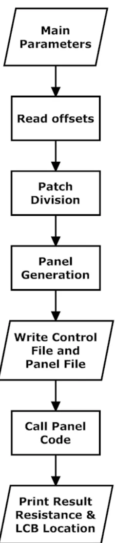
3 Methodology 11 3.1 Optimization Loop . . . 11
3.2 Objective Function . . . 12
3.3 Geometry Acquisition. . . 12
3.3.1 Geometry Input . . . 14
3.3.2 Panel Zones . . . 15
3.3.3 Panel Generation . . . 16
3.4 Panel Code . . . 19
3.5 Optimization Module . . . 19
3.5.1 Function . . . 19
3.5.2 Free Variable . . . 21
3.5.3 Shape Transformation . . . 21
4 Results 23 4.1 Input Data . . . 24
4.1.1 Geometry . . . 24
4.1.2 Panel Code . . . 25
4.2 Output. . . 28 4.2.1 Optimization Output . . . 28
5 Discussion 30
6 Conclusions 33
Bibliography 35
APPENDIX: Python code 37
List of Figures
2.1 Nelder Mead Simplex Flow Chart [3] . . . 10
3.1 Objective function flow chart . . . 13
3.2 Geometry file data points . . . 15
3.3 Different types of conventional vessels . . . 17
3.4 Panel points . . . 18
3.5 Optimizer Flow Chart . . . 20
3.6 Wave field output from panel code . . . 21
3.7 Top view: Wave field output from panel code . . . 22
4.1 SUSAN MAERSK - 6600 TEU Container Ship [1] . . . 25
4.2 Input geometry file . . . 26
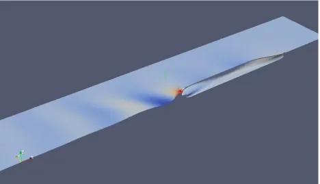
4.3 Waves generated along the ship’s length . . . 26
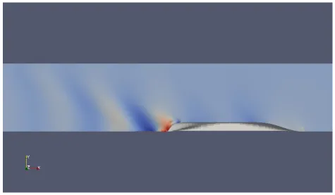
4.4 Waves generated at transom . . . 27
4.5 Optimization convergence at speed of 24 knots . . . 29
5.1 Kelvin wave angle . . . 31
5.2 Higher wave elevation at transom . . . 31
Nomenclature
α fraction for raise of free surface panels
¯
x centroid of half body as a fraction of halflength
¯
z LCB as a percentage of length
δz¯ required shift of LCB as a percentage of length
δφa required change in prismatic coefficient of afterbody
δφf required change in prismatic coefficient of forebody
δφt required change in total prismatic coefficient
δpa required change in length of aft parallel middle body
δpf required change in length of forward parallel middle body
δxa resultant longitudinal shift of aft section at xa
δxf resultant longitudinal shift of forward section at xf
φ prismatic coefficient of half body
φt total prismatic coefficient
A Lackenby constants for half body
Aa Lackenby constants for afterbody
Af Lackenby constants for forebody
B Lackenby constants for half body
Ba Lackenby constants for afterbody
Bf Lackenby constants for forebody
C Lackenby constants for half body
Cf Lackenby constants for forebody
k lever of the second moment of the original SAC about midships
LCB Longitudinal center of buoyancy from origin
p fractional length of parallel middle body of halflength
pa fractional length of parallel middle body of afterbody
pf fractional length of parallel middle body of forebody
SAC sectional area curve
xa co-ordinates from midhips to the aft end
xf co-ordinates from midhips to the forward end
Cm midship sectional area coefficient
Abstract
A ship must be designed for efficiency and economy, thus there is an everlasting desire for the design of better and better ships. One of the important factors which directly influence the worthiness of a design is its resistance. Throughout decades of ship design, the resistance is given top most importance as a design objective. With the increase in computational speeds of both software and hardware, there has been an opportunity for optimizing ship hulls using iterative methods of design and modification.
A method for calculating resistance for a given hull geometry and to optimize it using optimization algorithms are required for achieving better hulls. The resistance is calculated using a panel method for a given hull and the hull geometry is later changed by applying Lackenby’s method of longitudinal shift of stations.
An optimization algorithm extracts the best possible design out of the numerous design alternatives possible.
Keywords: Resistance, Panel Method, Lackenby Transformation, Optimization,
Chapter 1
Introduction
Development of new hull shapes is based on a number of coupled characteristic features.
They determine both technological and economic worthiness of a design. The development
of a new hull, in general, can be approached in three different ways:
• Hull form from standard series.
• Form parameter based hull design.
• Hull form generation based on parent ship data.
Hull form design based on standard series are derived from empirical data, such as Todd’s
Series 60 [2], Taylor Standard Series [16], BSRA [7], MARAD [13] and Ridgley-Nevitt [12],
resulted from model tests carried out in model basins. The individual models have been
derived from a parent hull by systematic variation of geometric parameters. In many of the
standard series length to beam ratio (L/B) and beam to draft ratio (B/T) have been varied.
Various methods have been proposed to select a hull form from the standard series data.
One of them is to select preliminary dimensions based on parent ship analysis. Parent ship
analysis is a deterministic approach where a new hull is selected by using regression analysis
on the available parent hull data. However, each of these series are developed for a specific
Form parameter based hull design starts with a very basic approach of using a small
num-ber of control parameters for attaining final design requirements. The basic hull properties,
such as center line buttock or the shape of the deck profile for example, are defined by curves
created from form parameters. Once this set of basic hull curves is created from the control
parameters, a numerical algorithm is applied to create a set of sections at selected locations.
This is achieved by utilizing a parametric curve generation process where the vertices of
all B-spline curves are computed from a geometric algorithm, which solves for a required
fairness criteria and a global shape constraints [17]. As the design is completely based on
the input form parameters, it may sometimes lead a designer into a techno-economically bad
design. Better hull forms can be generated by incorporating a design optimization method
within this design sequence.
The third alternative for designing hull forms is based on modifying an existing hull form.
This method gives a partial confidence to the designer right from the beginning as he starts
from a design which already performed well in real time. The selection of parent hull form
is based on a preliminary analysis of available vessels which are close to the desired hull
form with good design objectives. Even though the design is based on better parent hull
forms, they have to be optimized for the changes in operational conditions. For a ship hull
to be qualified as a good design, it has to meet the requirements such as minimal propulsion
power, maximum internal volume, maximum stability, ease of construction etc. [8].
1.1
Purpose, Motivation and Objective of Study
The rising demand for better transportation and latest development in computing power
has provided an opportunity to give automated design and optimization a thought. Efficient
transportation by sea plays a vital role in intercontinental trade. So for future transportation
we need a good design and optimization methods for achieving reliable hull forms. The
get better, whereas the optimization is the one which is yet to be developed for reliability
and validity. Thus a major consideration is given to the hull form optimization in present
work.
In the present work, a design optimization method is developed by taking a standard
hull of a KRISO container ship, provided by Korea Research Institute for Ships and Ocean
Engineering [14], and is used as a baseline model for verifying the results.
1.2
Proposed Method
The method comprises of geometry acquisition, panel generation, panel method for resistance
computation and the optimization. The process of hull optimization using a panel method
definitely requires a programming language with a higher computational power and a good
structure. To achieve the best out of available resources , FORTRAN is used for numerical
operations of panel method and PYTHON is used for reading geometry, panel generation
and integrating the process of optimization.
To make the process more generic, the hull geometry is considered as a standard GHS
geometry file format. This file typically contains markers which specify the sections of a hull.
The marker data is converted to a panel file using a shape function for panel distribution.
The aspect ratio of hull panels is also a significant factor contributing to the accuracy of the
panel method. The frictional resistance component remains almost the same and the major
component to be minimized, is the wave making resistance. The wave making resistance
is calculated by integrating the pressure distribution over wetted surface of the hull. It is
used as objective function in the optimization. The simple yet efficient Nelder-Mead simplex
algorithm is used for optimizing the hull for a better performance. The hull shape is varied
using the Lackenby [5] transformation respective to a change in LCB position.
At the end of the optimization process, the hull is iterated to reach an optimum LCB
Chapter 2
Background
2.1
Geometrical Variation of Ship Hull Forms
H. Lackenby [5] proposed a method of designing a new vessel by systematic geometric
vari-ation of a parent ship form. His alternative to the “one minus prismatic” method varies
the hull form with more control on design parameters. The “one minus prismatic” has a
few limitations for achieving control over the independent variation of prismatic coefficient
and parallel middle body, as well as restrictions on variation of fullness, entrance, run and
maximum longitudinal shift of sections [5]. Lackenby’s method allows to modify fullness,
longitudinal position of buoyancy, and the extent of parallel middle in both fore and after
bodies independently i.e. the variation can be carried in one or all of the above parameters
at a time. The method is as follows,
Lackenby Transformation
Many design evaluation methods, such as resistance calculation techniques, use the major
shape parameters of the hull to calculate their results. These parameters typically include
length, beam, draft, prismatic coefficient (Cp), longitudinal center of buoyancy (LCB), and
amidships coefficient (Cm). It is difficult to perform parametric or sensitivity studies using
time. For example, when a vessel’s length is varied, it’s Cp, LCB and displacement values
change at the same time. It would be desirable to be able to change any one of these major
design variables, while maintaining constant values for the rest. Of course, this is impossible,
because as one variable changes, at least one other variable must change to compensate. In
the present approach Lackenby method for my hull variation is used. This method used
the sectional area curve and allows for the modification of the following parameters The
following form parameters are varied. They are
• Prismatic coefficient (Cp)
• Longitudinal center of buoyancy (LCB)
• Parallel middle body - forward (pf)
• Parallel middle body - aft (pa)
δφf =
2 [δφt(Ba+ ¯z) + δz¯(φt+δφt)] + Cf ·δpf − Ca·δpa Bf +Ba
(2.1)
δφa =
2 [δφt(Bf −z¯) − δz¯(φt+δφt)] − Cf ·δpf + Ca·δpa Bf +Ba
(2.2)
For a required change in hull form, the sectional area distribution is changed. The
necessary change in station spacing is given by δxf for stations forward of midships and by
δxa for stations aft of midships.
δxf = (1−xf)
δpf
1−pf
+ (xf −pf)
Af
δφf −δpf
(1−φf)
(1−pf)
(2.3)
δxa = (1−xa)
δpa
1−pa
+ (xa−pa)
Aa
δφa−δpa
(1−φa)
(1−pa)
Where, the constants A, B and C are given by,
A = φ(1−2¯x)−p(1−φ) (2.5)
B = φ[2¯x−3k
2−p(1−2¯x)]
A (2.6)
C = B(1−φ)−φ(1−2¯x)
1−p (2.7)
The practical limits for variation in prismatic coefficient,δφf and δφa, to which the fullness
of a given from can be varied without resulting in a very steep sectional area curve at the
forward or aft ends is given by
δφ =
δp(1−φ)± 1 2A
1− 1δp−p
1−p (2.8)
The various constants involved in the above equations refer to either the fore or the aft
bodies as required. It is assumed that the reader has a basic knowledge of the coefficients
of form of a ship hull. Otherwise, a detailed explanation can be found in the Principles of
Naval Architecture, Vol 1 [6].
2.2
Effect of Variation in LCB
The effect of change in LCB position is very nominal upto a critical speed-length ratio, but
above this critical limit the variation of LCB is very prominent [11].
Effect on Resistance
The effect of increase in speed is very prominent on the resistance of a vessel. The optimum
position of LCB appears to move aft with increasing speed. Of course this depends on the
Other Effects
Changes in position of LCB seem to have less influence on the factors such as wake fraction,
thrust-deduction fraction, hull efficiency and quasi-propulsive coefficient. But as this
evalu-ation is done on a specific series of hull model, the effect can be validated as an optimizevalu-ation
constraint.
2.3
Panel Method
Boundary Element Method
In the last twenty years, the boundary-element method (BEM) has been established as a
powerful numerical technique for dealing with a variety of problems in science and engineering
involving elliptic partial differential equations. The strength of the method derives from its
ability to solve, with remarkable efficiency and accuracy, problems in domains with complex
and possibly evolving geometry where traditional methods can be inefficient, cumbersome,
or unreliable.
Various elements (elementary solutions) exist to approximate the disturbance effect of
the ship. These more or less complicated mathematical expressions are useful to model
displacements(sources) or lift(vortices or dipoles). The basic idea of all the related boundary
element methods is to superimpose elements in an unbounded fluid. Since the flow does not
cross a streamline just as it does not cross real fluid boundary (hull), any unbounded flow
field in which a stream line coincides with the actual flow boundaries in the bounded problem
can be interpreted as a solution for bounded flow problem in the limited fluid domain.
Panel Methods for computing the ship wave resistance in potential flow is one form of
a boundary element method where the ship hull is discretized into number of quadrilateral
and triangular panels with rankine sources distributed at each panel centre.
linearised free surface boundary condition are applied in the current version of the panel
method used. After solving for the source strengths at the panel centres. The pressure
distribution is then integrated to get the net forces acting on the body, which is the sum
of longitudinal force component, sinkage force and trimming moment of the ship moving
in fluid domain. In solving the potential flow, the free surface panels are raised above the
actual free surface to avoid singularities.
2.4
Optimization
Nelder Mead simplex, a simple yet efficient optimization algorithm is selected for this
prob-lem. The algorithm is very effective for the present probprob-lem. For the present case, it is a
known fact that the optimum LCB is located near the midships. So, the initial guess for the
optimization process is made at the midship.
2.4.1 Algorithm
The Nelder-Mead algorithm or simplex search algorithm, originally published in 1965 [9],
is one of the best known algorithms for multidimensional unconstrained optimization. The
basic algorithm is quite simple to understand and very easy to use. The method does not
require any derivative information, which makes it suitable for problems with non-smooth
functions. It is widely used to solve parameter estimation and similar statistical problems,
where the function values are uncertain or subject to noise. [15].
Even though the method is quite simple, it is implemented in many different ways. Apart
from some minor computational details in the basic algorithm, the main difference between
various implementations lies in the construction of the initial simplex, and in the selection
of convergence or termination tests used to end the iteration process. The general algorithm
1. Construct the initial working simplex.
2. Repeat the following steps until the termination test is satisfied.
3. Calculate the termination test information.
4. If the termination test is not satisfied then transform the working simplex.
5. Return the best vertex of the current simplex and the associated function value.
In many practical problems a highly accurate solution is not necessary and may be
im-possible to compute. All that is desired is an improvement in function value, rather than
full optimization. Though a true optimum is always better, there are limitations in lieu of
the computation time required.
The Nelder-Mead method frequently gives significant improvements in the first few iteration
and generally produces satisfactory results. Also, the method typically requires only one or
two function evaluations per iteration, except in shrink transformations. This is very
impor-tant in applications where each function evaluation is very expensive or time-consuming. For
such problems, the method is often faster than other methods, especially those that require
at least some function evaluations per iteration.
• Pro: In many numerical tests, the Nelder-Mead method succeeds in obtaining a good
reduction in the function value using a relatively small number of function
evalua-tions. Apart from being simple to understand and use, this is the main reason for its
popularity in practice.
• Con: The method can take an enormous amount of iterations with negligible
im-provement in function value, despite being nowhere near to a minimum. This usually
results in premature termination of iterations. A heuristic approach to deal with such
cases is to restart the algorithm several times, with reasonably small number of allowed
Chapter 3
Methodology
Hull shape optimization for a minimum resistance can be achieved using any of the geometric
variation processes as discussed in chapter2. However, our goal is to optimize ship hull with
a minimum deviation from the shape of the parent hull. For this reason, the variation of
LCB using Lackenby’s method of transformation [5] is considered appropriate.
3.1
Optimization Loop
The first step in the optimization loop is to read the hull geometry, where the hull offsets are
defined and boundary surfaces are discretized. Surface discretization has a direct influence
on the accuracy of any computational fluid dynamics solution. The ship hull geometry is
represented as a point distribution along the girth at every station on the hull surface. For
the purpose of discretization of hull surface into panels, the station spacing is changed and
controlled using a shape function. The panels are divided at every station and are equally
spaced girthwise. This kind of panel distribution will allow the optimization to work with
Lackenby transformation without the necessity for panel generation during each and every
iteration. Based on the type of the hull, subdivision of panels into zones is applied.
The second step is to find the resistance of the ship hull. This will serve as objective
for calculation of wavemaking resistance of the ship hull. The panel code is a FORTRAN 90
program which accepts a panel input file along with other control parameters.
Finally, the optimization process is carried out using a PYTHON module which uses the
Nelder - Mead simplex algorithm (section2.4) for control. The algorithm find the optimized
location of LCB for a particular speed.
3.2
Objective Function
The process of optimization iterates through the objective function (figure 3.1). The
func-tional value of wave making resistance is calculated by
• Reading hull geometry.
• Creating hull patches.
• Hull and free surface panel generation.
• Generating panel input and control files.
• Computing wave making resistance.
3.3
Geometry Acquisition
The hull surface has to be represented with a panel distribution of varying panel sizes. For
any computational fluid dynamics code to perform an accurate analysis, the panels have
to be distributed uniformly and uniquely concentrated at locations where the flow is more
complex. For a typical ship hull the flow near the bow and stern have large changes in flow
velocities. Thus a concentrated panel distribution is applied to the ends of the hull.
The hull is typically divided into four primary panel zones. The zones are divided
panel generation scheme, which can be generated using a linear interpolation or a Lagrangian
interpolation.
Panel zones maintain a consistent distribution by using a predefined global panel
distri-bution shape function. The zone division process can be applied to any typical hull geometry,
which are symmetric. Ships with a bulbous bow, transom stern, cruiser stern or centreline
propeller bossing can be handled effectively by the panel zone division.
3.3.1 Geometry Input
The hull surface is defined by a standard GHS geometry file which contains all the
infor-mation about the geometry of the vessel, represented in detail appropriate for hydrostatic
and stability calculations (figure3.2). It describes the volumes of the hull and various
com-partments. Each volume to be modelled consists of a series of transverse sections, arranged
from bow to stern. A geometry file can be generated either by manually typing offsets or by
using any other modelling software, Rhino3D is being used for this work. The geometry file
should have a centerline symmetric marker distribution without repeated values. Centerline
symmetric values can be defined on either port or starboard side.
Within the geometry file one or more components are defined together to form the
com-plete watertight hull surface. This surface is specified in the input to make the process of
hull generation more easier. Markers (offset points) in a geometry file are distributed along
every station and they are stored into a standard offset array.
The number of markers may or may not be the same for every station. So, a girth
wise subdivision is implemented to make them uniform. These offsets are stored in the offset
variable, of dimensions “ no. of points for a station×no. of stations×2 (for y and z)”. The
y offsets are represented in Array [ :, :, 0] and the corresponding z offsets in Array [ :, :, 1].
The offsets are passed through a sanity check to verify that they are increasing in height.
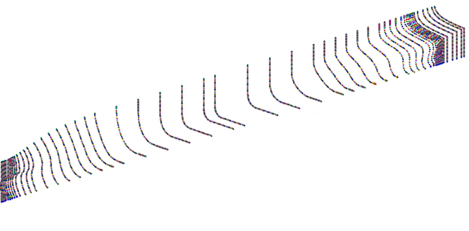
Figure 3.2: Geometry file data points
file for consistency.
3.3.2 Panel Zones
Every hull is divided into a four basic panel zones. This facilitates better way to generate
panels and representation. Panel zones are defined on the basis of boundary lines and hull
shape. Four variations in the zone distribution have been implemented for different types of
conventional vessels (figure 3.3):
• Type 1:
Center line propeller bosing - present.
Bulbous bow - present.
• Type 2:
Center line propeller bosing - absent.
Bulbous bow - present.
Center line propeller bosing - present.
Bulbous bow - absent.
• Type 4:
Center line propeller bosing - absent.
Bulbous bow - absent.
For each of the above cases the first zone will be the lower stern surface which includes
the bossing if present. The second zone will be the upper stern surface. Third zone will
be largest surface zone, the middle body surface. Last zone is defined for the bulbous bow
surface.
3.3.3 Panel Generation
Though panels can be generated from the predefined stations, a controlled variation of panel
distribution is essential for computational accuracy. A shape function is used to calculate and
control the new distribution of panel stations. Panel stations are generated by a simple local
interpolation of points in the three dimensional domain. Two approaches, linear interpolation
and Lagrangian interpolation, are considered for interpolating along the local domain.
Linear Interpolation
For every new station, two nearest stations are selected and a new y and z ordinates are
interpolated for the longitudinal (x ordinate) position of the station. As the stations are
equally divided along the girth, the number of interpolated points will be the same in each
station. Thus a vector interpolation is used to generate the same number of points at a
new station location. The interpolation is operated independently over each girth point of
same index along two selected stations. The two stations are adjacent to each other and are
Lagrangian Interpolation
This is a simple quadratic interpolation where three nearest stations are selected and an
approach similar to linear interpolation is used to find the Lagrangian interpolation
polyno-mials. For every new station location and for every girth interval, a new point is determined
from the Lagrangian interpolation polynomial.
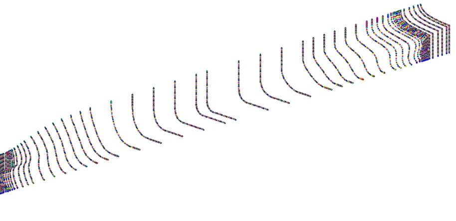
The old panel file (figure 3.2) is interpolated using any of the interpolation methods.
The new panel points are more structured and cleaned up as shown in fig 3.4. The
num-ber of points in the new stations depend on the required aspect ratio and the input file
specifications.
3.4
Panel Code
The Panel method is used for finding [4] a solution to the potential flow around a ship hull
(chapter2.3). The panel code developed by Dr. Lothar Birk is designed to run using a panel
file and a control file. The input panel file (*.pan) has a basic structure which first defines
length, symmetry condition, number of hull patches, number of free surface patches, total
number of hull points & panels and total number of free surface points & panels. The panel
zone location and orientation is also specified. All the points are specified and the detailed
orientation of every panel is listed.
The panel file is the most significant input that is defined after considering geometric
ap-proximations and appropriate free board panel raise. The rise in free board is specified by
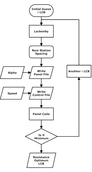
anα factor, which serves as a intermediate input for panel file generation (figure3.5).
3.5
Optimization Module
A typical optimization requires an optimization method and a function, which has to be
minimized. In this case the function is evaluated on the basis of resistance from panel code.
The function is designed to take LCB position as a free variable. The optimizer will thus
find the optimum LCB location at which the resistance is a minimum (figure 3.5).
3.5.1 Function
The function value is the coefficient of wave making resistance at a particular speed. This is
evaluated using panel code [4] which writes the output to an output file. This value is used
by the Nelder Mead simplex algorithm for its evaluations. The value of wave resistance will
become higher as we move away from the optimum point and there is only one optimum
location of LCB. The wave field created by the ship is sensitive to the panelization. The hull
Figure 3.6: Wave field output from panel code
3.5.2 Free Variable
Longitudinal Center of Buoyancy is one of the critical parameters which influence the wave
resistance of a ship moving in fluid domain. A general observation is that, at higher speeds
the LCB shifts towards aft and the contrary for slow speeds. This a very sensitive variable
which of course depends on the geometry and type of ship. So every ship has to be checked
for an optimum LCB for the design operation conditions. The functional change in wave
resistance for change in LCB is facilitated by changing hull form for required change in LCB
by using Lackenby transformation [5].
3.5.3 Shape Transformation
In the present work, only LCB is considered as a free variable. When the LCB is shifted
Figure 3.7: Top view: Wave field output from panel code
change in new station position, which is governed by Lackenby transformation method, thus
changing the panel file. The panel file is deigned to take station data and station spacing as
input. As the station location changes, the only change made is the station location input
Chapter 4
Results
The optimization of LCB position, for minimum wave resistance, using a panel method
(section3.3) was developed as a generic process. For the purpose of validation and discussion
a standard hull form [14] is considered for analysis. The results thus obtained are compared
with published technical data.
The optimization process has been carried out for a container ship hull of 53330 tons
displacement, advancing in calm water at a speed of 24 knots (Fn = 0.26) in fixed condition
(i.e., sinkage and trim not allowed). The optimization is applied only to the submerged hull.
Resistance due to wind and appendages are not taken into consideration. More precisely,
in the presented results the modification refers to just the submerged hull. Furthermore,
in the hull transformations, only the x-coordinate of the hull is allowed to vary, while the
4.1
Input Data
As discussed earlier in 3.3, the process can be categorised into three sections. Each of them
requires a specific input and they will generate output which will be passed on to the next.
The geometry acquisition reads the hull geometry file and it generates a panel file. The
panel code uses a panel file and a control file to generate the resistance. The resistance of
the ship hull respective to a particular LCB position serves as an objective function for the
optimization process.
4.1.1 Geometry
KRISO container ship (KCS) [14] is considered for analysis in this project. The KCS was
conceived to provide data for validation of flow physics and CFD for a modern container ship
with bulb bow and stern. Even though there is no existing ship exactly of same dimensions,
but a similar ship is operated for Maersk Lines, the SUSAN MAERSK (figure 4.1) which is
one of the largest container ship’s in the world.
Korea Research Institute for Ships and Ocean Engineering performed towing-tank
ex-periments to obtain resistance and wave field data for this ship. The data is available in the
KCS website [14].
Main Particulars
• Length between Perpendiculars, Lpp = 230.0 m
• Breadth, B = 32.2 m
• Depth, D = 19 m
• Draft, T = 10.8 m
Figure 4.1: SUSAN MAERSK - 6600 TEU Container Ship [1]
• Wetted surface area, Ω = 9424.0 m2
• Block Coefficient, Cb = 0.6505
• Mid ship section area coefficient, Cm = 0.9849
• Longitudinal center of buoyancy, LCB = -1.48 % of Lpp from midships
Offsets Data: The offset file of KRISO container ship is provided as an input, either a
GHS geometry file format or as a xyz offset data. The data provided has a distribution of
one hundred points at ever station (figure 4.2). These stations are interpolated using linear
interpolation along the length of the vessel. A numerical integration method is used for the
calculation of form parameters of the vessel.
4.1.2 Panel Code
The panel code reads the geometry from a panel file (*.pan) and control parameters from a
control file (*.in). A panel file is a detailed representation of all the panel points and their
Figure 4.2: Input geometry file
the input and the output files, Froude number, free surface condition, flow condition etc.
The code solves primarily for the pressure distribution. Later on wave making resistance,
stream lines and free surface deformation are evaluated. Post processing of these output files
is carried out using ParaView (figures 4.3 & 4.4).
Figure 4.3: Waves generated along the ship’s length
4.1.3 Optimization
As a basic optimization input a function to be optimized and an initial guess are defined.
Figure 4.4: Waves generated at transom
panel file which represents the hull is already generated from geometry acquisition module.
The panel stations are transformed using a lackenby transformation to achieve required LCB
position for the hull. The LCB position is the variable for the optimization problem and at
the end of optimization, an optimum location of LCB is determined.
Input for optimization module is:
• Speed, V = 24 knots
• Froude number, Fn = 0.26
• Parameter for raised panel height, α = 0.8
• Initial guess of LCB shift of -0.05 %(of half length of Lpp) from midships. This position
4.2
Output
Optimization algorithm searches for a optimum LCB position for a particular speed of ship.
The coefficient of resistance starts at an initial guess value and gradually converges to a
minimum (figure 4.5).
4.2.1 Optimization Output
• Number of Iterations = 9
• Total number of function evaluations = 19
• Minimum Coefficient of Wave Making Resistance, Cw = 0.00256509
• Optimized LCB location as a percentage of Lpp from midship = -1.65
Chapter 5
Discussion
1. LCB position: The location of optimized LCB is observed to be located aft of
mid-ships. This is as expected in view of hydrodynamics of a ship hull. The position of
LCB as provided in a Flow Vision document [10] is -1.48 % of Lpp from midship.
The observed value, -1.653 % of Lpp, is almost close to the published results and the
deviation of 0.17 % with respect to Lpp. This might be for the reasons that the hull
is approximated using linear panels.
2. Wave making resistance: The coefficient of wave making resistance, Cw = 0.002565,
is more than three times of what it actually should be, value of Cw = 0.000731 as
published [14].
There are a lot of assumptions involved in calculating the resistance such as linearized
free surface, geometry approximation using linear panels and the panel method itself.
But, they will not effect the determination of optimized LCB position. The
opti-mization algorithm only considers relative nature of resistance with change in LCB
position.
3. Wave pattern: The wave pattern fromed by the ship hull is in agreement with the
standard kelvin wave pattern with and half angle of 19.47 deg. The measured angle is
Figure 5.1: Kelvin wave angle
4. Transom wave profile: wave height at transom (figure 5.2) is higher than the
mea-sured wave profile data [14]. This is a general trend in panel methods for a ship hull.
Figure 5.2: Higher wave elevation at transom
trend (shifting towards aft) with increasing Froude number (figure 5.3). Further the
LCB is expected to shift towards aft.
Chapter 6
Conclusions
A generic method for optimization of ship hulls using panel method is presented. This
method uses a simple interpolation scheme to generate panels for any conventional ship hull.
The use of stations as a grid to develop panels eliminates the necessity to regenerate the
panels for every iteration. This resulted in a significant improvement in computational speed.
Lackenby transformation is used by the optimization algorithm to incorporate variation in
hull geometry for a required LCB shift. A simple, yet efficient Nelder - Mead simplex
method of optimization is used for this problem. In conclusion this approach has successfully
determined the optimum location of LCB for a standard container ship hull.
The obvious advantages of this method include the ability to represent any conventional
ship hull using a simple interpolation scheme for panel generation, an approximation which
is reliable. Also, the use of lackenby method of transformation enables a control over
pre-serving the volume and over all dimensions, while making a change in LCB position. The
optimization algorithm selected is also very efficient in solving this kind of a problem.
The results from this work concur with published data and theory. The present approach
focuses on locating an optimum LCB position for a ship hull and also observing the resistance
characteristics of a ship hull at different speeds. The key point is achieving a best design lies
in matching a ship hull with its operational conditions. The approach presented will enable
Further, the panel method can be extended to handle transom immersion, appendages,
trim and heel. The next milestone would be a panel code that includes non-linear free surface
conditions. The range of free variable of optimization has to be extended to bulbous bow
shape and also the over all dimensions. To add up, a stability approach would enhance the
Bibliography
[1] Susan maersk.
http://en.wikipedia.org/wiki/Emma_M%C3%A6rsk. vii, 25
[2] David W. Taylor Model Basin. and F. H. Todd. Series 60 methodical experiments with
models of single-screw merchant ships / by F. H. Todd. [Washington,, 1964. 1
[3] Lothar Birk. Name 6145 course notes. Fall 09. vii, 10
[4] Lothar Birk. Panel code: nlhsfs v0.8-uno academic license. 2009. 11, 19
[5] H. Lackenby. On the systematic geometrical variation of ship forms. INA, 92:289–315,
1950. 3,4, 11, 21
[6] Edward V. Lewis, editor. Principles of naval architecture, Written by a group of
au-thorities, volume 1, pages 32–33. Society of Naval Architects and Marine Engineers,
Jersey City, N.J., 1988. 6
[7] D. I. Moor, M. N. Parker, and R. N. M. Pattullo. The bsra methodical series: an overall
presentation. Transactions of the Royal Institution of Naval Architects, 103:329–419,
1961. 1
[8] Ebru Narli and Kadir Sari¨oz. Geometrical variation and distorsion of ship hull forms.
[9] J. A. Nelder and R. Mead. A simplex method for function minimization. The Computer
Journal, 7(4):308–313, January 1965. 8
[10] A. Pechenyuk. Computation of perspective kriso containership towing tests with the
help of the complex of hydrodynamical analysis flowvision. Technical report, 2009. 30
[11] G. J. Goodrich R. E. Blackwell and D. J. Doust. The effect on resistance and propulsion
of variation in lcb position. Transactions of the Royal Institution of Naval Architects,
99:367–406, 1957. 6
[12] C. RIDGLEY-NEVITT. The resistance of a high displacement-length ratio trawler
series. Transactions of the SNAME, 75, 1967. 1
[13] D. P. Roseman. Marad Systematic Series of Full Form Ship Models. Society of Naval
Architects and Marine Engineers, Jersy City, NJ, 1987. 1
[14] KRISO Container Ship. Gothenberg 2000.
http://www.iihr.uiowa.edu/gothenburg2000/KCS/container.html. 3, 23, 24, 30,
31
[15] A. Singer and J. Nelder. Nelder-mead algorithm. Scholarpedia, 4(7):2928, 2009. 8
[16] D. W. Taylor. Calculation of ship’s forms and the light thrown by model experiments
upon resistance, propulsion and rolling of ships. Transactions of the International
En-gineering Congress, 1915. 1
[17] Ping ZHANG, De xiang ZHU, and Wen hao LENG. Parametric approach to design of
Appendix: Python Source Code
1 # Mar 0 3 , 2010
# k k a r r i , H u l l s h a p e o p t i m i z a t i o n u s i n g l a c k e n b y t r a n s f o r m a t i o n
3 # and N e l d e r−mead s i m p l e x a l g o r i t h m
5 # i m p o r t i n g r e q u i r e d p a c k a g e s
7 import numpy a s np
from s c i p y . i n t e g r a t e import t r a p z , s i m p s
9 from s c i p y . i o import savemat
from s u b p r o c e s s import c a l l
11
# . . . Pre d e f i n e d f u n c t i o n s . . . .
13
def r e a d o f f s e t s ( f i l e n a m e , T) :
15 ”””
F u n c t i o n t o r e a d o f f s e t f i l e
17 I n p u t : f i l e n a m e o f o f f s e t s f i l e
T i s t h e d r a f t
19 Output : x l o n g = s t a t i o n s p a c i n g a l o n g x a x i s from AP
o f f s e t s = o f f s e t s s t o r e s h a l f b r e a d t h a s [ s t a t i o n number , h a l f
b r e a d t h , 0 ]
21 o f f s e t s s t o r e s h e i g h t a s [ s t a t i o n number , h e i g h t a b o v e
b a s e l i n e , 1 ]
23 ”””
f = open ( f i l e n a m e , ” r ” )
25 l i n e s = [ ]
d a t a = [ ]
27 o r i g i n a l l i n e s = f . r e a d l i n e s ( )
f o r l i n e in o r i g i n a l l i n e s :
29 l i n e = l i n e . s t r i p ( )
i f l i n e [ 0 ] ! = ”#” :
31 l i n e s . append ( l i n e )
f . c l o s e ( )
33
#c r e a t e s t o r a g e s p a c e f o r d a t a o f d i m e n s i o n ( number o f s t a t i o n s , no o f
p o i n t s , 2 )
35 o f f s e t s = np . z e r o s ( ( 5 7 , 1 0 0 , 2 ) , f l o a t )
37 # o f f s e t l i n e s r e a d f o r d a t a
# x l o n g i s l o n g i t u d i n a l d i s t a n c e o f s e c t i o n from AP,
39 x l o n g = [ ]
y s t = [ ]
41 z s t = [ ]
f o r i in np . l i n s p a c e ( 0 , 2 2 9 6 , 5 7 ) : # f o r r e a d i n g d a t a i n l i n e s
( 0 , 4 1 , 8 2 . . . . )
43 x l o n g . append ( f l o a t ( l i n e s [ i n t ( i ) ] . s p l i t ( ) [ 0 ] ) )
b = [ ]
45 h = [ ]
f o r j in np . l i n s p a c e ( 1 , 2 0 , 2 0 ) :
47 b . append ( l i n e s [ i n t ( i )+i n t ( j ) ] . s p l i t ( ) )
h . append ( l i n e s [20+ i n t ( i )+i n t ( j ) ] . s p l i t ( ) )
49
o f f s e t s [ i n t ( i / 4 1 ) , : , 0 ] = np . r e s h a p e ( b , np . s i z e ( b ) ) #b a s s i g n e d t o
51 o f f s e t s [ i n t ( i / 4 1 ) , : , 1 ] = np . r e s h a p e ( h , np . s i z e ( h ) ) #h a s s i g n e d t o
o f f s e t s
y s t . append ( o f f s e t s [ i n t ( i / 4 1 ) , : , 0 ] )
53 z s t . append ( o f f s e t s [ i n t ( i / 4 1 ) , : , 1 ] )
x l o n g = np . a s a r r a y ( x l o n g )
55
# A c r o s s s t o r e s S e c t i o n a l Area o f e a c h s t a t i o n
57 A c r o s s = [ ]
G i r t h = [ ]
59 f o r i in r a n g e ( 0 , 5 7 ) : # r u n s t h r o u g h a l l s t a t i o n s
A=0
61 f o r j in r a n g e ( 0 , 9 9 ) : # r u n s t h r o u g h a l l p o i n t s
# The c r o s s−s e c t i o n a l a r e a i s c a l c u l a t e d u p t o d r a f t
63 i f o f f s e t s [ i , j + 1 , 1 ] < T :
# f o r h < T, s e c a r e a i s c a l c u l a t e d by a d d i n g up a r e a o f
65 # Trapeziums
A = A + 2∗( ( o f f s e t s [ i , j + 1 , 1 ] − o f f s e t s [ i , j , 1 ] )∗0 . 5∗ \
67 ( o f f s e t s [ i , j , 0 ] + o f f s e t s [ i , j + 1 , 0 ] ) )
e l s e :
69 # b T = b p r e v i o u s +( d e l t a B / d e l t a h ) ∗ (T−b )
b T = o f f s e t s [ i , j , 0 ] +(( o f f s e t s [ i , j +1 ,0]−o f f s e t s [ i , j , 0 ] )\
71 ∗(T−o f f s e t s [ i , j , 1 ] ) / ( o f f s e t s [ i , j + 1 , 1 ] \
− o f f s e t s [ i , j , 1 ] ) )
73 A = A + 2∗( (T − o f f s e t s [ i , j , 1 ] )∗0 . 5∗ \
( o f f s e t s [ i , j , 0 ] + b T ) )
75 break
A c r o s s . append (A)
77
# g e n e r a t i n g o f f s e t a r r a y
79 #o f f s e t s s t o r e s h a l f b r e a d t h a s [ s t a t i o n number , h a l f b r e a d t h , 0 ]
81 y = o f f s e t s [ i , : , 0 ]
z = o f f s e t s [ i , : , 1 ]
83 # v = number o f p o i n t s a l o n g g i r t h w i s e
v = 99
85 d i s t = ( ( np . d i f f ( y ) )∗∗2 + ( np . d i f f ( z ) )∗ ∗2 )∗ ∗0 . 5
g i r t h = np . z e r o s ( l e n ( d i s t ) +1)
87 d e l t a = np . z e r o s ( v+1)
f o r k in r a n g e ( l e n ( d i s t ) ) :
89 g i r t h [ k +1] = g i r t h [ k ] + d i s t [ k ]
zpan = [ ]
91 ypan = [ ]
f o r k in r a n g e ( i n t ( v ) ) :
93 d e l t a [ k ] = sum ( d i s t )∗k/v
f o r j in r a n g e ( 1 , l e n ( g i r t h ) ) :
95 i f ( g i r t h [ j−1] <= d e l t a [ k ] ) &( g i r t h [ j ] > d e l t a [ k ] ) :
ypan . append ( y [ j−1] + ( ( y [ j ]−y [ j−1 ] )∗( d e l t a [ k]−g i r t h [ j−1 ] )
/\
97 ( g i r t h [ j ]−g i r t h [ j−1 ] ) ) )
zpan . append ( z [ j−1] + ( ( z [ j ]−z [ j−1 ] )∗( d e l t a [ k]−g i r t h [ j−1 ] )
/\
99 ( g i r t h [ j ]−g i r t h [ j−1 ] ) ) )
G i r t h . append ( g i r t h [−1 ] )
101 A c r o s s = np . a s a r r a y ( A c r o s s )
G i r t h = np . a s a r r a y ( G i r t h )
103
return x l o n g , o f f s e t s , y s t , z s t , A c r o s s , G i r t h
105
107 def p a t c h ( x l o n g , o f f s e t s , s t a , p , vp , r , v l , vu , sx , sy , s z , tx , ty , t z , bx , by , bz , beta , Lpp , T
) :
109 INPUT :
s t a : s t a t i o n number o r a r r a y . S p e c i f i e s s t a t i o n s o f a p a t c h
111 p : p a t c h number : 1−s t e r n t u b e ; 2−transom ; 3−h u l l body ; 4−b u l b
v : no o f p a n e l s g i r t h w i s e ??
113 r : ?
115 ”””
117 x = [ ]
y = [ ]
119 z = [ ]
121 i f p == 1 :
# p a t c h 1 ( s t e r n t u b e ) i s c l o s e d a t a f t end
123 f o r i in r a n g e ( v l +1) :
x . append ( s x )
125 y . append ( s y )
z . append ( s z )
127 i f p == 2 :
# p a t c h 2 ( transom ) i s c l o s e d a t a f t end
129 f o r i in r a n g e ( vu+2) :
x . append ( t x )
131 y . append ( t y )
z . append ( t z )
133 # p a t c h c l o s u r e a t t h e end f o r f r e e b o a r d p a n e l
z [−1 ] = ( t z + ( b e t a ∗ Lpp ) )
135
f o r i in s t a : # r u n s t h r o u g h a l l s t a t i o n s
137 z1 , y1 , y s t a r t , yend = s t a t i o n ( i , o f f s e t s , beta , Lpp , T)
ypan , zpan = s t a d i v ( z1 , y1 , y s t a r t , yend , p , vp , v l , vu , i , s t a [ 0 ] , 8 . 9 6 )
f o r j in r a n g e ( l e n ( ypan [ 0 ] ) ) :
141 x . append ( x l o n g [ i ] )
y . append ( ypan [ 0 ] [ j ] )
143 z . append ( zpan [ 0 ] [ j ] )
i f p == 2 :
145 i f np . s i z e ( y s t a r t ) == 1 :
f o r j in r a n g e ( l e n ( ypan ) ) :
147 x . append ( x l o n g [ i ] )
y . append ( ypan [ j ] )
149 z . append ( zpan [ j ] )
e l i f np . s i z e ( y s t a r t ) == 2 :
151 f o r j in r a n g e ( l e n ( ypan [ 1 ] ) ) :
x . append ( x l o n g [ i ] )
153 y . append ( ypan [ 1 ] [ j ] )
z . append ( zpan [ 1 ] [ j ] )
155 i f ( p== 3 ) | ( p ==4) :
f o r j in r a n g e ( l e n ( ypan ) ) :
157 x . append ( x l o n g [ i ] )
y . append ( ypan [ j ] )
159 z . append ( zpan [ j ] )
i f p == 4 :
161 # p a t c h 4 ( b u l b o u s bow ) i s c l o s e d a t fwd end
f o r i in r a n g e ( vp +1) :
163 x . append ( bx )
y . append ( by )
165 z . append ( bz )
return np . r o t 9 0 ( np . r e s h a p e ( x , (−1 , r +1) ) ,−1) ,\
167 np . r o t 9 0 ( np . r e s h a p e ( y , (−1 , r +1) ) ,−1) ,\
np . r o t 9 0 ( np . r e s h a p e ( z , (−1 , r +1) ) ,−1)−T
169
171 ”””
INPUT :
173 i = s t a t i o n number
OUTPUT:
175 z = a c t u a l s t a t i o n w a t e r l i n e s
y = a c t u a l s t a t i o n o f f s e t s
177 z 1 = s t a t i o n w a t e r l i n e s u p t o Load Water L i n e
y1 = s t a t i o n o f f s e t s u p t o Load Water L i n e
179 p = r e t u r n s t h e number o f d i s c o n t i n u o u s s e c t i o n s ( i . e . f o r transom p =2
a s t h e r e a r e two d i s c o n t i n u o u s s e c t i o n l i n e s
181 y s t a r t = s p e c i f i e s t h e s t a r t p o i n t s o f s e c t i o n s
yend = s p e c i f i e s t h e end p o i n t s o f s e c t i o n s
183
n o t e : S e c t i o n s a r e d e f i n e d a s c o n t i n u o u s s t a t i o n l i n e s ,
185 f o r e x a m p l e : transom s e c t i o n , s t e r n t u b e s e c t i o n , body s e c t i o n s ,
b u l b o u s bow s e c t i o n .
187 ”””
z = [ ]
189 y = [ ]
191 # T h i s l o o p s e l e c t s t h e submerged p o r t i o n o f t h e h u l l and f r e e b o a r d
#i . e . u p t o w a t e r l i n e and f r e e board , s t o r e s o f f s e t s i n y and z
193
f o r j in r a n g e ( 0 , 9 9 ) :# r u n s t h r o u g h a l l p o i n t s
195 i f o f f s e t s [ i , j , 1 ] < T :
z . append ( o f f s e t s [ i , j , 1 ] )
197 y . append ( o f f s e t s [ i , j , 0 ] )
199 e l s e :
b T = o f f s e t s [ i , j , 0 ] +(( o f f s e t s [ i , j +1 ,0]−o f f s e t s [ i , j , 0 ] )\
− o f f s e t s [ i , j , 1 ] ) )
203 z . append (T)
y . append ( b T )
205
# f o r f r e e b o a r d o f f s e t s
207 f b = b e t a ∗ Lpp
T f b = T + f b
209 j = np . n o n z e r o ( o f f s e t s [ i , : , 1 ] >= T f b ) [ 0 ] [ 0 ] −1
b f b = o f f s e t s [ i , j , 0 ] +(( o f f s e t s [ i , j +1 ,0]−o f f s e t s [ i , j , 0 ] )\
211 ∗( T fb−o f f s e t s [ i , j , 1 ] ) / ( o f f s e t s [ i , j + 1 , 1 ] \
− o f f s e t s [ i , j , 1 ] ) )
213 z . append ( T f b )
y . append ( b f b )
215 break
217 # y1 ans z 1 r e t u r n s t h e v a l u e s o f i n t e r p o l a t e d v a l u e s u p t o WL
z1 = [ ]
219 y1 = [ ]
# t h i s i s r e t u r n e d w i t h a v a l u e s p e c i f y i n g no . o f p a t c h e s
221 y s t a r t = [ ]
yend = [ ]
223 f o r k in r a n g e ( 1 , l e n ( z ) ) :
i f ( y [ k ] > 0 . ) & ( y [ k−1] == 0 . ) :
225 y s t a r t . append ( k−1)
yend . append ( l e n ( z )−1)
227 y1 . append ( y [ k−1 ] )
z1 . append ( z [ k−1 ] )
229 y1 . append ( y [ k ] )
z1 . append ( z [ k ] )
231 e l i f ( y [ k ] > 0 . ) & ( y [ k−1] >0.) :
233 z1 . append ( z [ k ] )
e l i f ( y [ k ] == 0 . ) &( y [ k−1] >0.) :
235 yend [ l e n ( yend )−1] = k
y1 . append ( y [ k ] )
237 z1 . append ( z [ k ] )
return z1 , y1 , y s t a r t , yend
239
def s t a d i v ( z1 , y1 , y s t a r t , yend , p , v , v l , vu , i , bs , tb ) :
241 ”””
T h i s f u n c t i o n d i v i d e s a s e c t i o n i n t o e q u a l p a t c h e s
243
INPUT :
245 z 1 = w a t e r l i n e s p a c i n g
y1 = h a l f b r e a d t h
247 y s t a r t = s p e c i f i e s t h e s t a r t p o i n t s o f s e c t i o n s
yend = s p e c i f i e s t h e end p o i n t s o f
249 p = no . o f p a t c h e s
v = number o f p a t c h e s i n v e r i c a l d i r e c t i o n
251 i = s t a t i o n number
b s = s t a t i o n number a t b u l b c l o s i n g , g e n e r a l l y s t a [ 0 ]
253 t b = trimming d r a f t a t b u l b , p o i n t s a b o v e t b a r e n e g l e c t e d i n b u l b p a t c h
255 OUTPUT:
ypan and zpan a r e t h e o f f s e t s f o r t h e p a n e l p o i n t s
257 ”””
# d i v i s i o n f o r s t a t i o n s w i t h c o n t i n i o u s s e c t i o n s
259 i f ( np . s i z e ( y s t a r t ) == 1 ) | ( p == 3 ) :
ypan , zpan = g i r t h d i v ( v , y1 , z1 , 1 )
261 # d i v i s i o n f o r b u l b s e c t i o n s
i f p == 4 :
# t h i s l i n e makes t h e b u l b an a p p r o x i m a t e c y l i n d e r
265 up = np . n o n z e r o ( np . a r r a y ( z1 )>tb ) [ 0 ] [ 0 ]
ypan , zpan = g i r t h d i v ( v , y1 [ : up ] , z1 [ : up ] , 0 )
267 e l s e:
ypan , zpan = g i r t h d i v ( v , y1 , z1 , 0 )
269 # d i v i s i o n when t h e r e a r e d i s c o n t i n i o u s s e c t i o n s
e l i f ( np . s i z e ( y s t a r t ) == 2 ) & ( p != 3 ) &(p ! = 4 ) :
271 y 1 l = y1 [ 0 : yend [ 0 ]−y s t a r t [ 0 ] + 1 ]
y1u = y1 [ yend [ 0 ]−y s t a r t [ 0 ] + 1 : l e n ( y1 ) ]
273 z 1 l = z1 [ 0 : yend [ 0 ]−y s t a r t [ 0 ] + 1 ]
z1u = z1 [ yend [ 0 ]−y s t a r t [ 0 ] + 1 : l e n ( z1 ) ]
275
# f o r l o w e r p a t c h
277 ypanl , z p a n l = g i r t h d i v ( v l , y 1 l , z 1 l , 0 )
# f o r u p p e r p a t c h
279 ypanu , zpanu = g i r t h d i v ( vu , y1u , z1u , 1 )
281 ypan = [ ypanl , ypanu ]
zpan = [ z p a n l , zpanu ]
283 return ypan , zpan
285 def g i r t h d i v ( v , y2 , z2 , wl ) :
”””
287 T h i s f u n c t i o n d i v i d e s any g i v e n s e c t i o n p a t c h i n t o number o f e q u a l
p a n e l s . The c a l c u a t i o n o f p a t c h l e n g t h i s b a s e d on t h e l e n g t h a l o n g g i r t h
289
INPUT :
291 v = number o f p a t c h e s i n v e r i c a l d i r e c t i o n
y2 = h a l f b r e a d t h
293 z 2 = w a t e r l i n e s p a c i n g
295 OUTPUT:
ypan and zpan a r e t h e o f f s e t s f o r t h e d i v i d e d s e c t i o n p a t c h e s
297 ”””
i f wl == 0 :
299 y = y2
z = z2
301 e l s e:
y = y2 [ :−1 ]
303 z = z2 [ :−1 ]
d i s t = ( ( np . d i f f ( y ) )∗∗2 + ( np . d i f f ( z ) )∗ ∗2 )∗ ∗0 . 5
305 g i r t h = np . z e r o s ( l e n ( d i s t ) +1)
d e l t a = np . z e r o s ( v+1)
307 f o r i in r a n g e ( l e n ( d i s t ) ) :
g i r t h [ i +1] = g i r t h [ i ] + d i s t [ i ]
309 zpan = [ ]
ypan = [ ]
311 f o r i in r a n g e ( i n t ( v ) ) :
d e l t a [ i ] = sum ( d i s t )∗i /v
313 f o r j in r a n g e ( 1 , l e n ( g i r t h ) ) :
i f ( g i r t h [ j−1] <= d e l t a [ i ] ) &( g i r t h [ j ] > d e l t a [ i ] ) :
315 ypan . append ( y [ j−1] + ( ( y [ j ]−y [ j−1 ] )∗( d e l t a [ i ]−g i r t h [ j−1 ] ) /\
( g i r t h [ j ]−g i r t h [ j−1 ] ) ) )
317 zpan . append ( z [ j−1] + ( ( z [ j ]−z [ j−1 ] )∗( d e l t a [ i ]−g i r t h [ j−1 ] ) /\
( g i r t h [ j ]−g i r t h [ j−1 ] ) ) )
319 zpan . append ( z [−1 ] )
ypan . append ( y [−1 ] )
321 i f wl==1:
zpan . append ( z2 [−1 ] )
323 ypan . append ( y2 [−1 ] )
return ypan , zpan
327
def s t a i n t e r p ( x l o n g , zone , p a n d i s t , npan , x , y , z ) :
329 # number o f p o i n t s f o r new s t a t i o n s
n l e n = l e n ( x )
331
n s t a= s t a g e n ( zone , p a n d i s t , npan )
333
nx= np . z e r o s ( [ l e n ( x ) , l e n ( n s t a ) ] , f l o a t )
335 ny= np . z e r o s ( [ l e n ( x ) , l e n ( n s t a ) ] , f l o a t )
nz= np . z e r o s ( [ l e n ( x ) , l e n ( n s t a ) ] , f l o a t )
337
d e s c e n d i n g = 0
339 i f np . any ( np . d i f f ( x [ 0 ] )<0) :
d e s c e n d i n g = 1
341 x = x [ : , : :−1 ]
y = y [ : , : :−1 ]
343 z = z [ : , : :−1 ]
345 f o r i in r a n g e ( l e n ( n s t a ) ) :
347 i f n s t a [ i ] > x [ 0 ] [−1 ] :
x f l o o r = l e n ( x ) − 1
349 e l s e:
x f l o o r = np . s e a r c h s o r t e d ( x [ 0 ] , n s t a [ i ] )
351
x l = x [ : , x f l o o r ]
353 x r = x [ : , x f l o o r −1]
y l = y [ : , x f l o o r ]
355 y r = y [ : , x f l o o r −1]
357 z r = z [ : , x f l o o r −1]
359 f o r j in r a n g e ( l e n ( x ) ) :
d e l t a = ( ( x r [ j ]−x l [ j ] )∗∗2 + ( y r [ j ]−y l [ j ] )∗∗2 + \
361 ( z r [ j ]−z l [ j ] )∗ ∗2 )∗ ∗0 . 5
t = ( n s t a [ i ]−x l [ j ] )∗( d e l t a / ( x r [ j ]−x l [ j ] ) )
363 nx [ j , i ] = n s t a [ i ]
ny [ j , i ] = y l [ j ]+ ( t∗( ( y r [ j ]−y l [ j ] ) / d e l t a ) )
365 nz [ j , i ] = z l [ j ]+ ( t∗( ( z r [ j ]−z l [ j ] ) / d e l t a ) )
367 i f d e s c e n d i n g == 1 :
nx = nx [ : , : :−1 ]
369 ny = ny [ : , : :−1 ]
nz = nz [ : , : :−1 ]
371
return nx , ny , nz
373
def s t a g e n ( zone , p a n d i s t , npan ) :
375 ”””
I n p u t :
377 z o n e = [ a f t e x t , fwd e x t , x s t a r t , xend ]
a f t and fwd e x t a r e t h e e x t r e m e p o i n t s on t h e h u l l
379 x s t a r t i s where t h e f i r s t s t a t i o n s t a r t s , xend i t where i t e n d s
p a n d i s t = P an e l d i s t r i b u t i o n a r r a y − [ [−1 . 0 ,−. 9 ,−0 . 2 5 , 0 . , 0 . 2 5 , 0 . 9 , 1 . 0 ] ,\
381 [ 0 . 0 , 0 . 2 5 , 1 . 0 , 1 . 0 , 1 . 0 , 0 . 2 5 , 0 . 0 ] ]
383 F i r s t row − l o n g i t u d i n a l a x i s ( n o r m a l i z e d
Second row r e p r e s e n t s t h e v a r i a t i o n o f p a n e l l e n g t h form a f t t o
fwd ,
385 npan = number o f p a n e l s p o i n t s
387 n s t a = n o r m a l i z e d new s t a t i o n s i n t h e s p e c i f i e d z o n e
389 ”””
x = np . l i n s p a c e ( min ( p a n d i s t [ 0 ] ) , max ( p a n d i s t [ 0 ] ) , 1 0 0 )
391 y = np . i n t e r p ( x , p a n d i s t [ 0 ] , p a n d i s t [ 1 ] )
A = [ ]
393 f o r i in r a n g e ( l e n ( x ) ) :
A. append ( t r a p z ( y [ 0 : i + 1 ] , x [ 0 : i + 1 ] ) )
395 A = np . a r r a y (A)
zx = np . i n t e r p ( np . l i n s p a c e ( z o n e [ 2 ] , z o n e [ 3 ] , npan ) ,\
397 np . l i n s p a c e ( z o n e [ 0 ] , z o n e [ 1 ] , 1 0 0 ) , x )
n s t a = np . i n t e r p ( zx , x ,A)
399 # N o r m a l i z e d
n s t a = n s t a / ( n s t a [−1]−n s t a [ 0 ] )
401 n s t a = n s t a − min ( n s t a )
n s t a = z o n e [ 2 ] + ( n s t a ∗ abs ( z o n e [ 3 ]−z o n e [ 2 ] ) )
403
return n s t a
405
def v i s u a l ( x , y , z , p , d i s p ) :
407
#s a v e f i n a l p a t c h o f f s e t s t o ∗. a r r
409 savemat ( ’ x ’+s t r ( p )+ ’ . mat ’ , mdict={’ a r r ’ : x})
savemat ( ’ y ’+s t r ( p )+ ’ . mat ’ , mdict={’ a r r ’ : y})
411 savemat ( ’ z ’+s t r ( p )+ ’ . mat ’ , mdict={’ a r r ’ : z})
413 i f d i s p == 1 :
# To v i e w t h e p a n e l s g e o m e t r y w i t h MATLAB
415 f i g = p l t . f i g u r e ( )
ax = Axes3D ( f i g , a s p e c t = ’ a u t o ’ )
from m a t p l o t l i b import cm
419 from m p l t o o l k i t s . mplot3d import Axes3D
import m a t p l o t l i b . p y p l o t a s p l t
421 # c r e a t i n g s u r f a c e p l o t
ax . p l o t s u r f a c e ( x , y , z , r s t r i d e = 1 , c s t r i d e = 1 , cmap = cm . j e t )
423 # s t a r b o a r d s i d e o f h u l l
ax . p l o t s u r f a c e ( x,−y , z , r s t r i d e = 1 , c s t r i d e = 1 , cmap = cm . j e t )
425 ax . s e t x l a b e l ( ’X ’ )
ax . s e t y l a b e l ( ’Y ’ )
427 ax . s e t z l a b e l ( ’ Z ’ )
429 def p a t c h f s ( xwl , ywl , f s p a n , v f s , T, Lpp , Lwl , d e l t a s , beta , w b e t a ) :
”””
431 i n i t i a l f r e e s u r f a c e p o i n t s g e n e r a t i o n
433 INPUT :
x w l : x c o r d i n a t e s o f w a t e r l i n e
435 y w l : y c o o r d i n a t e s o f w a t e r l i n e
f s p a n : Number o f Free s u r f a c e p a n e l s f o r one s h i p l e n g h t
437 v f s : t r a n s v e r s e number o f p a n e l
Lpp : L e n g t h b e t w e e n P e r p e n d i c u l a r s
439 d e l t a s : F a c t o r t o d e t e r m i n e i n i t i a l p a n e l o f f s e t from H u l l w a t e r l i n e
( ˜ 0 . 0 1 5 )
441 w b e t a : Rate o f i n c r e a s e i n p a n e l w i d t h away from h u l l . ( ˜ 1 . 1 )
”””
443 #Lwl l o c a l
x f s 0 = np . l i n s p a c e ( xwl [ 0 ] + ( 0 . 5∗Lwl ) , xwl [−1 ]−( 1 . 5∗Lwl ) , ( 3∗f s p a n ) +1)
445 x f s = np . t i l e ( x f s 0 , ( v f s +1 ,1) )
# number o f p a n e l s on WL, l e n g t h w i s e
447 s f s = np . s h a p e ( x f s ) [ 1 ] −1
449 y f s 0 = np . i n t e r p ( x f s 0 [ ( 0 . 5∗f s p a n ) :−( ( 1 . 5∗f s p a n ) +1) ] [ : :−1 ] ,\
xwl [ : :−1 ] , ywl [ : :−1 ] ) [ : :−1 ]
451 #a t t a c h i n g p a n e l s fwd
y f s 0 = np . append ( np . z e r o s ( 0 . 5∗f s p a n ) , y f s 0 )
453 #a t t a c h i n g p a n e l s a f t
y f s 0 = np . append ( y f s 0 , np . z e r o s ( ( 1 . 5∗f s p a n ) +1) )
455 y f s = [ ]
d e l t a = ( np . v a n d e r ( [ w b e t a ] , v f s +1)∗Lpp∗d e l t a s ) . s q u e e z e ( )
457
f o r i in r a n g e ( l e n ( y f s 0 ) ) :
459 s c a l e = ( sum ( d e l t a )− y f s 0 [ i ] ) / sum ( d e l t a )
d e l t a 1 = s c a l e ∗ d e l t a [ : :−1 ]
461 y f s . append ( y f s 0 [ i ] )
f o r j in r a n g e ( 1 , v f s ) :
463 y f s . append ( d e l t a 1 [ j ]+ y f s [−1 ] )
y f s . append ( d e l t a s∗w b e t a∗Lpp∗(1− w b e t a∗ ∗( v f s ) ) / ( 1 −w b e t a ) )
465
y f s = np . a r r a y ( y f s ) . r e s h a p e ( s f s +1 , v f s +1) . T
467 z f s = np . z e r o s ( ( v f s +1 , s f s +1) )
f b = b e t a ∗ Lpp
469 z f s [ . . . ] = T+ f b
471 return x f s , y f s , z f s−T
473 def r e s i s t a n c e ( x0 ) :
”””
475 T h i s f u n c t i o n c a l c u l a t e s t h e r e s i s t 5 a n c e f o r t h e m o d i f i e d h u l l form
by dLCB
477 ”””
d e s c = 0
d e s c = 1
481 x p a r e n t = nx3 [ : , : : −1 ] [ 0 , : ]
483 s a c p a r e n t = np . i n t e r p ( x p a r e n t , x l o n g , A c r o s s )
# d i s t a n c e o f f i r s t s t a t i o n from A. P .
485 min xp = min ( x p a r e n t )
# m o d i f y i n g x p a r e n t t o h a v e f i r s t s t a t i o n a t x = 0
487 x p a r e n t = x p a r e n t − min xp
489 # P a r t 2 : M o d i f y i n g H u l l form
x d e r i v e d , s a c p a r e n t , CPa , Cpf , pf , CP, LCB = \
491 l a c k e n b y ( x p a r e n t , s a c p a r e n t , dpa =0 , d p f =0 ,dCP=0 , dLCB = x0 )
# m o d i f y i n g x d e r i v e d t o g e t b a c k t o normal s t a t e i . e . f i r s t s t a t i o n a t
493 # x = min xp
i f d e s c == 1 :
495
x d e r i v e d = x d e r i v e d [ : :−1 ] + min xp
497 e l s e:
499 x d e r i v e d = x d e r i v e d + min xp
501 # P a r t 3 : C a l c u l a t e r e s i s t a n c e u s i n g Dr . B i r k ’ s p a n e l c o d e
R = panelmethod ( x d e r i v e d , f i l e n a m e , o r i g i n , Lpp , Lwl , nx1 , nx2 , nx2t , nx3 , nx4 , nx5
,\
503 ny1 , ny2 , ny2t , ny3 , ny4 , ny5 , nz1 , nz2 , nz2t , nz3 , nz4 , nz5 , f s p a n , v f s , T, d e l t a s
, beta , w b e t a )
505 # P a r t 4 : C o n s t r a i n t a p p l i c a t i o n
## e v a l u a t e c o n s t r a i n t s f o r p e n a l t y f u n c t i o n
509 # c o n s t r a i n t s
c . append ( l c b r a n g e (LCB, x p a r e n t [−1 ] ) )
511
# c o n v e r t t h e l i s t t o a numpy a r r a y ( f o r f a s t e r math )
513 c = np . a s a r r a y ( c )
515 # D e f i n e and compute e x t e r i o r p e n a l t y f u n c t i o n
r = 1 . e1 0
517 ”””
M u l t i p l i c a t i o n by a huge number
519 ”””
P = np . sum ( c∗c )
521
print ” L o n g i t u d i n a l c e n t e r o f Buoyancy , LCB = %12.12 f ”%LCB
523 print ’ R e s i s t a n c e , R = %12.12 f ’%R
print ’ P e n a l t y f u n c t i o n , r∗P = %f ’ % ( r∗P)
525 print ”\n”
f p = open ( ” o p t i m i z a t i o n ”+s t r ( Vs )+ ’ ’+s t r ( a l p h a )+” . d a t ” , ’ a ’ )
527 f p . w r i t e ( ’ %12.12 f %12.12 f\n ’ % (LCB, R) )
f p . c l o s e ( )
529 return R + r∗P
531 def l a c k e n b y ( x p a r e n t , s a c p a r e n t , dpa , dpf , dCP , dLCB) :
533 # p a r a l l e l mid boy d a t a
p = 0 . 0 # t o t a l l e n g t h o f p a r a l l e l midbody / h a l f l e n g t h
535 pa = 0 . 0 0 # p a r . midbodz a f t o f m i d s h i p / h a l f l e n g t h
p f = p − pa # p a r . midbodz f o r w a r d o f m i d s h i p / h a l f l e n g t h
537
#e x t r a c t p a r e n t h u l l d a t a
![Figure 2.1: Nelder Mead Simplex Flow Chart [3]](https://thumb-us.123doks.com/thumbv2/123dok_us/8946010.1855378/21.612.144.469.153.639/figure-nelder-mead-simplex-flow-chart.webp)


![Figure 4.1: SUSAN MAERSK - 6600 TEU Container Ship [1]](https://thumb-us.123doks.com/thumbv2/123dok_us/8946010.1855378/36.612.75.540.102.305/figure-susan-maersk-teu-container-ship.webp)