in the population sciences published by the Max Planck Institute for Demographic Research Konrad-Zuse Str. 1, D-18057 Rostock · GERMANY www.demographic-research.org
DEMOGRAPHIC RESEARCH
VOLUME 24, ARTICLE 18, PAGES 409-454
PUBLISHED 11 MARCH 2011
http://www.demographic-research.org/Volumes/Vol24/18/ DOI: 10.4054/DemRes.2011.24.18
Research Article
A new relational method for smoothing and
projecting age specific fertility rates:
TOPALS
Joop de Beer
© Joop de Beer 2011.This open-access work is published under the terms of the Creative Commons Attribution NonCommercial License 2.0 Germany, which permits use, reproduction & distribution in any medium for non-commercial purposes, provided the original author(s) and source are given credit.
1 Introduction 410
2 Methods for fitting age-specific fertility rates 411
2.1 Parametric models 412
2.2 Splines 414
2.3 Relational methods 416
3 TOPALS 418
4 Smoothing age-specific fertility rates 420
5 Scenarios 430
5.1 Projections based on a time series model 430 5.2 Scenarios based on qualitative assumptions 437
6 Conclusion and discussion 442
7 Acknowledgements 445
References 446
A new relational method for
smoothing and projecting age-specific fertility rates:
TOPALS
Joop de Beer1
Abstract
Age-specific fertility rates can be smoothed using parametric models or splines. Alternatively a relational model can be used which relates the age profile to be fitted or projected to a standard age schedule. This paper introduces TOPALS (tool for projecting age patterns using linear splines), a new relational method that is less dependent on the choice of the standard age schedule than previous methods. TOPALS models the relationship between the age-specific fertility rates to be fitted and the standard age schedule by a linear spline. This paper uses TOPALS for smoothing fertility age profiles for 30 European countries. The use of TOPALS to create scenarios of the future level and age pattern of fertility is illustrated by applying the method to project future fertility rates for six European countries.
1 Netherlands Interdisciplinary Demographic Institute, PO Box 11650, NL 2502 AR The Hague.
1. Introduction
In order to make population projections, assumptions need to be based on the future values of age-specific fertility rates in addition to assumptions about mortality and migration. Due to random fluctuations in fertility rates over time, assumptions based on extrapolation from past changes in each age-specific fertility rate tend to result in erratic age patterns. Moreover such a procedure does not take into account the fact that changes in fertility rates which are caused by changes in the timing of fertility are temporary. Postponement of fertility will first lead to a decline in age-specific fertility rates at young ages, then some time later to an increase at older ages. After a certain period the decline at young ages will come to an end, then some time later the increase at older ages will stop. Thus past trends will not continue forever. For these reasons assumptions about future fertility may be based on a parameterized model age schedule rather than by projecting individual age-specific fertility rates separately. The parameters of the model schedule may reflect the level and timing of fertility. This means that the model schedule can be used to make assumptions about the extent to which both the level and the timing of fertility may change. A large number of model age schedules for fertility have been developed. One reason why so many models have been developed is that most of them do not accurately describe age patterns of fertility for all countries in all periods.
There are two main criteria for assessing the usefulness of a method for smoothing age profiles: the accuracy of the fit of the model to the data and the possibility of interpreting the values of the parameters. There is a trade-off. As many model age schedules turn out not to provide a very accurate description of the age pattern for all ages, the model may be adjusted by the introduction of additional parameters. However, this may hamper the interpretation. Non-parametric methods, such as splines, are more flexible than parametric models and are therefore capable of describing all kinds of age patterns. However, they lack interpretable parameters. One alternative approach is to use a relational method: that is, a method in which the age pattern is related to one standard age schedule. The function specifying this relationship indicates the way in which the age pattern under study differs from the standard age schedule.
parameters are not enough. This article introduces the new relational method TOPALS (tool for projecting age patterns using linear splines), which is more flexible than the Brass method, produces a better fit, and is easier to interpret.
TOPALS is capable of describing all kinds of age curves. The parameters can be interpreted easily. TOPALS models the age pattern of the ratios of the age-specific rates to be fitted and the standard age schedule by a linear spline. The standard age pattern may be the average age pattern of a group of countries (e.g., the EU average). For making projections, this may be useful if one assumes future convergence of age-specific fertility rates of different countries to an average pattern. It is also possible to use the age pattern of another country as standard. This may be a “forerunner” country and one may assume that the age-specific fertility rates of different countries will move in the direction of that of the forerunner country. Alternatively the standard age pattern may be a model age schedule, such as the Hadwiger, Beta, or Gamma function. TOPALS can be used for making projections of future changes in age-specific rates by specifying assumptions about changes in the values of the ratios of the age pattern to be projected and the standard age schedule for successive age intervals. For example, if the standard age schedule is that of a forerunner country, one can assume that the future values of the rate ratios for other countries will move towards one.
The second section of this article presents a short overview of previous studies on modelling age patterns. We distinguish between parametric models, splines and relational methods. Section 3 describes TOPALS. Section 4 applies TOPALS in order to smooth age patterns of fertility for 30 European countries. The results of TOPALS are compared with those for six other methods. Section 5 describes how TOPALS may be used for creating scenarios of future values of age-specific fertility rates. Section 6 concludes the article and discusses some other possible applications of TOPALS.
2. Methods for fitting age-specific fertility rates
There is an extensive literature on parametric age schedules describing the typical age
pattern of fertility (e.g.,Hoem et al. 1981; Rogers 1986; Booth 2006; Peristera and
assumptions about future fertility as an input for population projections. One alternative is to specify a spline in such a way that the parameters can be interpreted (Schmertmann 2003). Another is to develop a relational model in which the age pattern of a given country is related to a standard age schedule. The relationship specifies the way in which the age pattern differs from the standard age schedule.
2.1 Parametric models
This section describes the three most frequently used parametric models for fitting fertility age patterns: the Hadwiger, Beta and Gamma models (Hoem et al. 1981; Booth 2006). In addition a recently developed parametric method will be discussed (Peristera and Kostaki 2007).
One of the earliest models proposed in the literature is the Hadwiger function (Yntema 1969; Gilje 1972; Hoem et al. 1981). This function is described by
)} 2 (
exp{ )
( 2 2
3
− + − ⎟ ⎠ ⎞ ⎜ ⎝ ⎛ =
c x x c b x
c c ab x
f , (1)
where f(x) is the fertility rate at age x of the mother and a, b, and c are the three
parameters to be estimated. Parameter a is associated with the total level of fertility,
parameter b determines the height of the curve, and parameter c is related to the mean
age at motherhood. Even though the parameters have a demographic interpretation, they indicate a direction of change only and their actual values are not directly interpretable.
A higher value of a indicates that the total fertility level is higher. But the value of a
does not equal the value of the total fertility rate (TFR). For example, in fitting the Hadwiger function to age-specific fertility rates in 30 European countries in 2008, we
find that a ranges from 0.75 in Hungary (where the TFR equals 1.35) to 1.24 in Iceland
(where the TFR equals 2.15). A linear regression of the values of a and the TFR shows
that TFR equals 1.76*a. The value of c turns out to be very close to the mean age at
childbearing. The value of ab/c is related to the modal age-specific fertility rate
(Chandola, Coleman, and Hiorns 1999), but this does not make the value of b itself
ethnic differences in the timing and level of fertility. They distinguish two subpopulations with a different timing and level of fertility. They describe this pattern by a mixture model: That is, they replace the right-hand side of equation (1) by the weighted sum of two similar terms which describe the age patterns of the two subpopulations.
The Gamma function is given by
(
)
exp{ ( )}) ( 1 ) ( 1 c d x d x c b R x
f b − b − −
Γ
= − for x > d, (2)
where R determines the level of fertility and d the minimum age at childbearing. The
Gamma function is equivalent to the Pearson Type III model which was applied by
George et al. (2004) to Canadian data. Hoem et al. (1981) show how the parameters b
and c are related to the mode, mean, and variance of the function but not in a simple,
linear way and so they do not have a direct demographic interpretation. The Beta function is given by
(
)
( 1)( ) 1( ) 1) ( ) ( ) ( − − + − − − − − Γ Γ + Γ
= A B A B
x x a x
B A
B A R
f β α β for α<x<β, (3)
where R determines the level of fertility. The Beta function is equivalent to the Pearson
Type I curve proposed by Romaniuk (1973) and Mitra and Romaniuk (1973). Hoem et
al. (1981) state that α and β represent lower and upper age limits of fertility, but
Peristera and Kostaki (2007) show that in several cases the value of β far exceeds the
maximum age. Hoem et al. (1981) show that A and B are related to the mean and
variance, but not in a simple, easily interpretable way.
Peristera and Kostaki (2007) note that the form of the fertility curve has changed in recent years in various countries, as did Chandola, Coleman, and Hiorns (1999) before them. Peristera and Kostaki (2007) propose a flexible model that describes both the standard and the distorted age-specific fertility pattern in countries such as the United Kingdom, Ireland, and Spain. Their basic model resembles the normal distribution but is asymmetrical, as the spread before and after the peak differs:
} )2 ) ( ( exp{ ) ( 1 x x c x f σ μ − −
= , (4)
where σ(x) = σ11 if x ≤ µ and σ(x) = σ12 if x > µ and c1, µ, σ11 and σ12 are the parameters
to be estimated. The parameter c1 is associated with the TFR, µ is the modal age of
respectively. In order to fit fertility curves with high fertility at a young age Peristera and Kostaki (2007) add a second term:
} ) ( exp{ }
) ( exp{ )
( 2
2 2 2
2 1
1
1 σ
μ σ
μ −
− +
− −
=c x c x
x
f , (5)
where c1 and c2 reflect the level of fertility at the first and second peak respectively, µ1
and µ2are related to the mean age of the two subpopulations, and σ1 and σ2reflect the
spread around the two humps. Even though the parameters are related to the level, mean age, and spread of the fertility curve, the actual values of the parameters are difficult to interpret. For example, in fitting model (4) to fertility data from various European
countries the estimate of c1 varies from 0.09 in Italy to 0.15 in Denmark. Although there
is a positive correlation between c1 and the TFR, the correlation is certainly not perfect.
If model (4) is estimated for 30 European countries, the value of c1 explains not more
than 80% of the variance in the TFR across European countries. Gayawan et al. (2010) propose the adjusted error model for modelling age-specific fertility rates in African
countries. This model is very similar to equation (5); they assume c1 = c2 and add an
intercept to the model.
One conclusion that applies for all parametric models is that even though the values of the parameters are related to the level, mean age, and variance of the functions, the values are not equal to well-known demographic indicators such as the TFR and the mean age at childbearing. This hampers interpretation of the parameters and limits their usefulness for creating demographic scenarios. Moreover one simple model with a limited number of parameters does not describe adequately the variety of age patterns of fertility across countries in different periods. Therefore several complex models including more parameters are needed.
2.2 Splines
fertility curves. Brass (1960, 1975) fits third-degree polynomials to describe the age pattern of fertility. The fit of the third-degree polynomial is less accurate than that of a cubic spline, which is a piecewise cubic function (Hoem et al. 1981). Cubic splines are very flexible (McNeil, Trussell, and Turner 1977; Gilks 1986). A cubic spline can be described by
∑
= − − + − + − + = n j j j j x m k Dd m x c m x b a x f 1 3
2 ( )
) ( ) ( )
( , (6)
where Dj= 0 if x – m≤ kj and Dj= 1 otherwise, m is the minimum age, x ≥ m, kj are the
knots, n is the number of knots, and a, b, c, and dj are the coefficients to be estimated.
A quadratic spline is a piecewise quadratic function that can be described by
∑
= − − + − + = n j j j j x m k Dc m x b a x f 1 2 ) ( ) ( )
( , (7)
where Dj= 0 if x – m≤ kj and Dj= 1 otherwise, m is the minimum age, x ≥ m, kj are the
knots, n is the number of knots, and a, b, and cj are the coefficients to be estimated.
Both a quadratic and a cubic spline can provide a good fit. In general a quadratic spline may require more knots than a cubic spline to provide an accurate fit. For both the quadratic and cubic splines, the coefficients can be estimated by Ordinary Least Squares (OLS) if the knots are fixed a priori. Otherwise an iterative estimation procedure is needed: for example, a non-linear least squares method.
Kostaki et al. (2009) propose a new non-parametric method: support vector machines (SVM). Even though this provides a good fit, its usefulness for projecting age-specific fertility rates seem limited. SVM models are more complex than splines. Since quadratic and cubic splines are capable of producing a good fit as well, the question is why use SVMs rather than splines.
quadratic spline in such a way that the resulting function describes the typical form of the fertility curve. The Schmertmann method improves the usefulness of splines for making projections. However, it is questionable whether one of the indicators, the age at which fertility falls to half its peak level, really has an obvious demographic interpretation. One general conclusion is that non-parametric models provide a better fit than parametric models. The latter are smoother and thus are not capable of describing various specific patterns at certain ages. However, the usefulness of non-parametric methods for making projections or creating scenarios is limited, as they lack easily interpretable parameters.
2.3 Relational methods
Fertility age schedules can be fitted by specifying how the age-specific fertility rates in a particular country deviate from some standard age schedule. Coale and Trussell (1974) modelled age-specific marital fertility rates as the product of two model age schedules: a nuptiality schedule and a marital fertility schedule. The parameters of the model indicate to what extent the age-specific fertility rates for a particular country deviate from the model age schedules. In the 1970s this model performed rather well (Hoem et al. 1981; Rogers 1986). However, since the 1980s extramarital fertility has increased in many countries. For that reason the usefulness of modelling marital fertility has decreased.
Brass (1974) presents a more general relational method in which fertility rates can be related to any fertility age schedule as long as it captures the general shape of the age pattern of fertility to be fitted. The Brass relational method is based on the assumption that the (cumulative) age pattern of fertility can be described by the Gompertz distribution. This implies that the log-log transformation of the rates to be fitted is linearly related to age. As the Gompertz distribution provides a reasonable fit except at extreme ages, Brass proposed to improve the fit by using a standard age schedule. Assuming that this standard age schedule can be described by a Gompertz distribution as well, there is a linear relationship between the log-log transformation of the rates to be fitted and that of the standard age schedule
*
x
Q β
x
Q =α+ , (8)
where Qx= ln− (−lnf(x)) and Qx*=−ln( ln− f *(x)); f(x) are the age-specific fertility
rates to be fitted and f *(x) are the fertility rates according to the standard age schedule.
The parameters αand β can be estimated by OLS regression. Even though the basic
distribution, Brass and others have shown that various types of age profile may be used as the standard age schedule, including observed rates from another country, as long as the standard schedule represents the general age pattern of the rates to be fitted (Zeng et al. 2000). In addition to using the relational model as an instrument for making projections, the model can also be used for making estimates of age-specific rates for
countries with incomplete data. The parameters α andβ can be interpreted as follows:
α determines the location of fertility and β the spread. Thus α indicates whether the
age pattern lies to the right or left of the standard age schedule and β determines
whether the age pattern is more or less dispersed than the standard.
Zeng et al. (2000) note that even though the parameters α andβcan be
interpreted, in practice they do not turn out to be very useful for making projections of
demographic rates for the future. The main reason is that the values of α andβ are not
comparable over time and regions, as they depend on the choice of the standard age schedule, and in order to have an optimal fit the choice of standard age schedules may
vary across time and space. Moreover changes in the values of α andβ lack a clear
demographic interpretation. They indicate the direction of change only. For example, if
the age curve is assumed to move to the right, the value of α should become larger.
But it is not clear by how much. For that reason Zeng et al. (2000) propose an
alternative method for the estimation of αandβ . They show that the value ofβ equals
the ratio of the interquartile ranges of the standard age schedule and that of the age
pattern to be fitted. The value of αis related to the median age. Zeng et al. demonstrate
that this model is capable of describing various unimodal age patterns: namely, fertility, first marriage, divorce, remarriage, and leaving the parental home. They use Chinese, French, Swedish, and US data. They use the model for fitting age patterns based on both a standard age pattern from an earlier period and a standard pattern from another country.
One main advantage of the method proposed by Zeng et al. is its simplicity. Once an appropriate standard age schedule is available, one needs to estimate the values of only two parameters. One problem is that the goodness of fit depends heavily on the choice of the standard age schedule. If the age pattern to be fitted differs from the pattern of the standard age schedule in some age range, the two parameters are not sufficient to adjust the curve to produce an overall good fit. Therefore different standard age schedules may have to be used at different points in time, which makes it difficult to use this method to extrapolate changes over time.
differs from the standard age schedule in successive age intervals. Since for different points in time the parameters may refer to the same standard age schedule they can be used for analysing changes over time and therefore become the basis for extrapolations into the future.
3. TOPALS
We assume that a standard age schedule of fertility rates is given. The age profile for a given country can be estimated on the basis of ratios of the age-specific fertility rates of
that country and those according to the standard age schedule. The rate ratio at age x is
) ) ) (x r = 0 b ( ( * x f x f
, (9)
where f *(x) is the fertility rate at age x according to the standard age schedule. The age
pattern of the ratios can be described by a linear spline function. This is a piecewise linear curve. The ages at which the successive linear segments are connected are called “knots”. The ratios at each age can be estimated by the linear spline function
∑
= − − + − + = n j j j j x m k D b m x b a x r 10( ) ( )
) (
ˆ , (10)
where Dj= 0 if x – m≤ kj and Dj= 1 otherwise, m is the minimum age, x ≥ m, kj are the
knots, n is the number of knots, and a and bj are the parameters to be estimated.
This model can be estimated in several ways. The knots can be fixed a priori: for example, on the basis of visual inspection of the age pattern of the rate ratios. Alternatively they can be chosen in such a way that the fit of the linear spline to the data is optimal. In the latter case a non-linear estimation method is required: for example, a
non-linear least squares method. If the location of the knots is fixed a priori, a and bj
can be estimated by OLS. However, these parameter values are difficult to interpret as they indicate the slopes in the successive age intervals rather than the levels at specific
ages. In the first age interval, m,…, k1, the slope equals â+) ; in the second age
interval, k1+1,…, k2, the slope equals â+b0
)
+b1
)
, etc. It is much easier to interpret the levels of the rate ratios at specific ages than the successive slopes in the age intervals.
Thus from the regression estimates one can calculate the values of at the knots.
These can be used as a basis for making projections. Alternatively the linear spline can be estimated in a more simple and straightforward way by assuming that at the knots
) (
ˆ x
the values of the spline equal the observed values. It turns out that this provides a fit that is very close to the one produced by applying OLS. We therefore assume that
= , =r , = , etc. Then the values of a, bj can be estimated
by substituting the values of , , , etc. in (10). This yields:
) (
ˆm
r r(m)
a
) ( ˆ k1
r (k1) rˆ(k (
ˆm
r
)
2 r(k2)
) rˆ(k1) rˆ(k2)
) =r(m)
m k m r − − 1 ) ( ) k r b = 1
0 ( ) (11)
∑
= − j i i b 1 ˆ ) −1 ( ˆ r + + − − j j j j k k k r 1 1) () ( )
(x f* x
= j
k r
b) ( .
For the ages above the last knot we assume that the slope equals zero. Alternatively one might assume that the slope above the last knot equals that before the last knot. Since fertility rates at high ages are small, this choice hardly affects the results. In contrast, when using TOPALS to fit other schedules, such as age-specific mortality schedules, this choice would make a difference. In those cases it is an empirical question which choice one would make.
The age-specific fertility rates are estimated by multiplying the ratios which are
estimated by the linear spline function by the age-specific fertility rates according
to the model age schedule f *(x):
) x
ˆ ) (
ˆ x r
f = . (12)
In the application of TOPALS in the next section we will select the knots by
minimizing the sum of squared differences between and f(x) by means of a
non-linear least squares method. We apply a grid search where for each set of knots we
calculate the values of a and bj by solving equation (11) rather than by applying OLS.
) (
ˆ x
f
rates of the forerunner country. A partial adjustment model can be used to project the future values of the rate ratios. This can be considered as a quite “objective” method. The choice of the “target” values of the age-specific fertility rates may be subjective, but the parameter of the partial adjustment model estimated for some historical period determines how rapidly the rate ratios will move towards one and thus whether the age-specific fertility rates will reach the “target” values before some age-specific forecast horizon. Second, one may follow a more subjective approach by making assumptions about the future values of the rate ratios for selected ages based on qualitative arguments. For example, if the standard age schedule is the average pattern over a number of countries, for each separate country one may make assumptions about the extent to which one assumes that the fertility rates at different age ranges will remain different from the average or will move towards the average values. In Section 5 we will demonstrate both procedures for using TOPALS to create scenarios.
4. Smoothing age-specific fertility rates
We illustrate the use of TOPALS by fitting age-specific fertility rates for 30 European countries: the 27 EU countries (Austria, Belgium, Bulgaria, Cyprus, Czech Republic, Denmark, Estonia, Finland, France, Germany, Greece, Hungary, Ireland, Italy, Latvia, Lithuania, Luxembourg, Malta, the Netherlands, Poland, Portugal, Romania, Slovakia, Slovenia, Spain, Sweden, and the United Kingdom) plus Iceland, Norway, and Switzerland. We label these 30 European countries as the EU27+3 countries. The data are obtained from the database of Eurostat, which is available online (Eurostat 2010). At the time of writing data for 2008 were available for 27 countries. For Italy the most recent data were from 2007, for the United Kingdom from 2006, and for Belgium from 2005.
We calculated unweighted and weighted averages of age-specific fertility rates for the EU27+3 countries. Rather than using total population size of each country as weights, we calculated the weighted average by weighing the fertility rates for each country by the number of women aged 15–44 years. The TFR based on the unweighted average of the EU27+3 countries equals 1.61, while that based on the weighted average equals 1.58.
The values of the TFR range from 1.32 in Slovakia to 2.15 in Iceland. Most countries in southern, central and eastern Europe have a TFR between 1.3 and 1.5, whereas most northern and western European countries have a TFR above 1.6. In the remainder of this article we will use weighted averages.
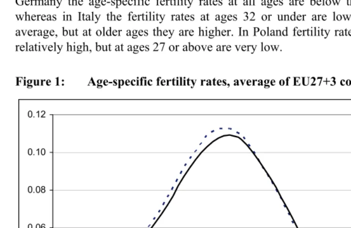
Germany and Italy, have relatively low fertility rates among women in their 20s or early 30s, the peak of the weighted average age pattern of fertility rates is lower than that of the unweighted average. Figure 2 compares age-specific fertility rates of six European countries with the average of the EU27+3: Denmark, France, Germany, Italy, Poland, and United Kingdom,. These countries are selected as they reflect differences in the level and age pattern of fertility rates in different parts of Europe. The three northern and western countries, Denmark, the United Kingdom, and France, have an above average TFR. But there are clear differences in the age pattern of fertility rates across these three countries. Whereas in Denmark fertility rates at young ages (under 23 years) are below the European average, those in the United Kingdom are significantly higher. The age patterns of Denmark and France are much more peaked than that of the United Kingdom. The peak in France is at slightly younger ages than the European average. The other three countries, Germany, Italy, and Poland, have below average TFR. In Germany the age-specific fertility rates at all ages are below the European average, whereas in Italy the fertility rates at ages 32 or under are lower than the European average, but at older ages they are higher. In Poland fertility rates at younger ages are relatively high, but at ages 27 or above are very low.
Figure 1: Age-specific fertility rates, average of EU27+3 countries, 2008
0.00 0.02 0.04 0.06 0.08 0.10 0.12
15 17 19 21 23 25 27 29 31 33 35 37 39 41 43 45 47 49
Figure 2: Age-specific fertility rates of six European countries, compared with the EU27+3 average, 2008
Denmark 0.00 0.02 0.04 0.06 0.08 0.10 0.12 0.14 0.16
15 17 19 21 23 25 27 29 31 33 35 37 39 41 43 45 47 49
United Kingdom 0.00 0.02 0.04 0.06 0.08 0.10 0.12 0.14 0.16
15 17 19 21 23 25 27 29 31 33 35 37 39 41 43 45 47 49
France 0.00 0.02 0.04 0.06 0.08 0.10 0.12 0.14 0.16
15 17 19 21 23 25 27 29 31 33 35 37 39 41 43 45 47 49
Germany 0.00 0.02 0.04 0.06 0.08 0.10 0.12 0.14 0.16
15 17 19 21 23 25 27 29 31 33 35 37 39 41 43 45 47 49
Italy 0.00 0.02 0.04 0.06 0.08 0.10 0.12 0.14 0.16
15 17 19 21 23 25 27 29 31 33 35 37 39 41 43 45 47 49
Poland 0.00 0.02 0.04 0.06 0.08 0.10 0.12 0.14 0.16
15 17 19 21 23 25 27 29 31 33 35 37 39 41 43 45 47 49
Solid line: observed values; dotted line: EU27+3 average
Note: Observed values for the United Kingdom refer to 2006 and for Italy to 2007.
The average age at childbearing of the EU27+3 countries equals 29.2 years. If in a country the mean age at childbearing is higher than the European average this can be caused by low fertility rates at young ages (e.g., Italy), by a relatively high peak of fertility around age 30 (Denmark), or by high fertility rates at older ages (France). A low level of the mean age can be caused by high fertility rates at young ages (e.g., the United Kingdom) or low fertility rates at older ages (Poland).
Figure 3: Rate ratios of age-specific fertility rates of six European countries and EU27+3 average, 2008
Denmark 0.00 0.20 0.40 0.60 0.80 1.00 1.20 1.40 1.60 1.80 2.00
15 17 19 21 23 25 27 29 31 33 35 37 39 41 43 45 47 49
United Kingdom 0.00 0.20 0.40 0.60 0.80 1.00 1.20 1.40 1.60 1.80 2.00
15 17 19 21 23 25 27 29 31 33 35 37 39 41 43 45 47 49
France 0.00 0.20 0.40 0.60 0.80 1.00 1.20 1.40 1.60 1.80 2.00
15 17 19 21 23 25 27 29 31 33 35 37 39 41 43 45 47 49
Germany 0.00 0.20 0.40 0.60 0.80 1.00 1.20 1.40 1.60 1.80 2.00
15 17 19 21 23 25 27 29 31 33 35 37 39 41 43 45 47 49
Italy 0.00 0.20 0.40 0.60 0.80 1.00 1.20 1.40 1.60 1.80 2.00
15 17 19 21 23 25 27 29 31 33 35 37 39 41 43 45 47 49
Poland 0.00 0.20 0.40 0.60 0.80 1.00 1.20 1.40 1.60 1.80 2.00
15 17 19 21 23 25 27 29 31 33 35 37 39 41 43 45 47 49
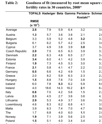
The linear splines shown in the figure are fitted by calculating equation (11). The knots are selected by applying a non-linear least squares method to data for the 30 European countries in this study. For all countries the same knots are selected. This makes cross-country comparisons easier. Linear splines based on minimum age 15 years and five knots (ages 19, 24, 29, 34, and 40 years) turn out to fit the observed rate ratios accurately. Table 1 shows the values of the rate ratios at these ages for all 30
countries. The root mean square error (RMSE) equals 2.83 x 10⁻³ (see Table 2). If four
knots are selected the fit is clearly less accurate: the RMSE equals 3.20 x 10⁻³.
However, for some countries four knots would be sufficient. The selection of a knot at age 19 is needed to capture the relatively high level of fertility at young ages in countries such as the United Kingdom and Poland, but it would not be needed for fitting the age schedule in, for example, Denmark. Similarly a knot at age 40 would not be needed for providing a good fit for the United Kingdom or France. Thus, when fitting a spline for a single country, the minimum number of knots needed for providing an accurate fit may be fewer than five. For 13 out of the 30 European countries the fit of the model including four knots – that is, without a knot at age 19 – would be about equal to that of the model including five knots. Adding knots obviously improves the fit of the model. However, adding a sixth knot turns out to produce only a slight
improvement of the fit. Adding a knot at age 27 yields a RMSE of 2.60 x 10⁻³. Since a
Table 1: Values of the rate ratios of age-specific fertility rates of European countries and EU27+3 average at knots, total fertility rate (TFR) and mean age at childbearing (MAC), 2008*
15 19 24 29 34 40 TFR MAC
Austria 0.57 0.85 0.99 0.91 0.85 0.81 1.41 29.0
Belgium 0.51 0.87 1.24 1.35 0.95 0.71 1.76 28.8
Bulgaria 8.52 2.03 1.30 0.76 0.53 0.37 1.47 26.1
Cyprus 0.36 0.64 0.92 1.01 0.94 0.92 1.46 29.7
Czech Republic 0.44 0.85 1.00 1.15 0.82 0.63 1.50 28.8
Denmark 0.10 0.56 1.05 1.44 1.34 1.18 1.89 29.9
Estonia 1.28 1.45 1.26 0.94 0.89 0.98 1.65 28.3
Finland 0.12 0.84 1.18 1.24 1.20 1.27 1.85 29.6
France 0.54 0.89 1.33 1.40 1.18 1.24 2.00 29.4
Germany 0.54 0.71 0.85 0.89 0.94 0.90 1.38 29.6
Greece 1.45 0.83 0.89 0.98 1.03 0.98 1.51 29.6
Hungary 2.13 1.12 0.83 0.90 0.74 0.63 1.35 28.4
Iceland 0.00 1.26 1.46 1.40 1.22 1.46 2.15 29.3
Ireland 0.58 1.35 0.95 1.03 1.74 2.25 2.10 30.7
Italy 0.04 0.52 0.69 0.83 1.06 1.29 1.37 30.5
Latvia 1.06 1.62 1.30 0.80 0.63 0.72 1.44 27.6
Lithuania 0.91 1.34 1.27 0.97 0.64 0.51 1.47 27.7
Luxembourg 0.00 0.73 0.88 1.03 1.11 1.06 1.61 30.0
Malta 1.50 1.01 0.96 1.00 0.85 0.56 1.44 28.7
The Netherlands 0.25 0.43 0.93 1.30 1.36 0.97 1.77 30.2
Norway 0.17 0.83 1.32 1.35 1.26 1.05 1.96 29.4
Poland 0.54 1.20 1.14 0.91 0.63 0.57 1.39 28.0
Portugal 1.53 0.99 0.81 0.85 0.88 0.85 1.37 29.1
Romania 5.23 1.86 1.11 0.75 0.50 0.42 1.35 26.4
Slovakia 1.63 1.31 0.97 0.86 0.63 0.48 1.32 27.8
Slovenia 0.08 0.37 1.02 1.23 0.91 0.67 1.53 29.4
Spain 1.06 0.89 0.67 0.79 1.19 1.24 1.46 30.3
Sweden 0.18 0.55 1.14 1.32 1.35 1.29 1.91 30.1
Switzerland 0.19 0.39 0.78 0.97 1.19 1.15 1.48 30.5
United Kingdom 1.16 1.77 1.22 1.03 1.09 1.14 1.84 28.7
EU27+3 average 1.58 29.2
Table 2: Goodness of fit (measured by root mean square error) of age-specific fertility rates in 30 countries, 2008*
TOPALS Hadwiger Beta Gamma Peristera- Schmertmann Brass Brass
RMSE
Kostaki** OLS
Non-linear LS (x 10-3
)
Average 2.8 7.9 5.9 6.4 3.2 3.6 6.6 3.5
Austria 1.3 5.7 3.6 3.8 2.1 2.6 3.8 1.4
Belgium 3.3 5.9 5.2 4.8 3.2 3.3 9.3 3.2
Bulgaria 6.1 6.2 5.7 4.2 2.5 3.6 6.0 2.3
Cyprus 3.7 4.9 3.8 3.9 3.0 3.4 8.9 3.3
Czech Republic 2.0 7.5 6.5 6.3 3.9 3.3 7.2 3.5
Denmark 2.2 6.3 4.6 6.5 2.7 3.4 4.5 2.2
Estonia 3.4 6.0 4.1 4.2 3.9 4.4 6.2 4.5
Finland 1.9 7.3 4.5 5.3 3.0 3.3 4.3 2.1
France 2.1 5.8 4.1 4.7 2.2 2.5 6.7 3.4
Germany 0.5 6.6 4.2 4.9 1.5 2.2 1.4 0.7
Greece 2.0 8.2 5.9 6.3 2.3 2.2 4.8 1.8
Hungary 1.5 8.8 7.6 7.0 3.8 2.9 4.2 3.4
Iceland 6.0 7.8 5.3 6.2 5.9 6.6 15.2 7.8
Ireland 4.0 18.6 14.3 16.2 2.1 6.4 15.7 8.1
Italy 0.8 7.0 4.2 5.6 1.5 2.2 3.0 0.9
Latvia 2.3 4.5 2.7 3.6 3.6 4.1 6.2 4.2
Lithuania 2.9 5.3 4.9 3.7 3.6 3.0 4.4 3.5
Luxembourg 4.6 8.3 6.2 6.8 4.1 3.9 6.5 3.6
Malta 3.9 8.3 7.4 7.0 4.7 3.8 5.0 4.8
The 1.7 6.8 4.0 6.0 1.1 2.0 4.5 1.4
Norway 1.9 7.1 3.9 5.6 2.5 3.0 3.3 2.3
Poland 1.5 5.1 4.0 3.4 3.4 2.7 5.2 2.0
Portugal 1.3 8.8 6.8 6.9 4.1 2.9 3.1 2.1
Romania 2.5 6.5 5.7 5.1 4.1 3.9 4.7 1.5
Slovakia 1.4 7.5 6.4 5.6 3.6 2.9 6.3 2.1
Slovenia 2.0 5.2 4.0 4.0 3.0 3.0 6.7 2.4
Spain 2.1 11.8 9.2 10.3 0.8 3.3 7.5 5.0
Sweden 2.5 7.9 4.9 6.5 3.0 3.0 2.8 2.1
Switzerland 1.1 6.8 3.8 5.4 1.7 1.9 1.8 1.6
United Kingdom 2.2 11.3 8.1 8.7 2.1 5.9 4.9 3.2
Number of
parameters 5 4 3 4 4 4 2 2
* For Italy data refer to 2007, for the United Kingdom to 2006, and for Belgium to 2005 ** Model 2 applied to Ireland, Spain, and the United Kingdom
Multiplying the linear splines shown in Figure 3 by the (weighted) EU27+3 average fertility rates shown in Figure 1 produces the TOPALS fertility age schedule for each country. Figure 4 shows that TOPALS is capable of describing different age patterns of fertility, each based on the same standard age schedule. The model is capable of describing the relatively high fertility at young ages in the United Kingdom and Poland. Figures A1–A4 in the Appendix show the fit of TOPALS for the other 24 European countries. For most countries the fit is satisfactory. One exception is Bulgaria, where the fitted curve is not smooth at young ages. This is caused by the fact that the rate ratios for Bulgaria at young ages do not exhibit a linear shape between ages 15 and 19. This implies that an additional knot between these ages would be needed to obtain a smooth curve. If a knot at age 17 is added the fit improves considerably. Furthermore the fit for Belgium and Ireland can be improved by adding a knot at age 27.
It is interesting to compare the results obtained using TOPALS with those obtained using other relational and parametric models. First, we compare the results of TOPALS with those of the three most frequently applied parametric models: the Hadwiger, Gamma and Beta functions. On average the Beta function produces a better fit than the other two models. This confirms the results obtained by Peristera and Kostaki (2007). Hoem et al. (1981) compared a great variety of methods for smoothing fertility age patterns by applying them to Danish fertility data in the 1970s. They concluded that the Gamma and Hadwiger functions performed better than the Beta distribution. Peristera and Kostaki (2007) note that the unsatisfactory fit of the Beta model by Hoem et al. (1981) may be due to the fact that they had problems in obtaining least squares estimates of the coefficients of the Beta distribution. Peristera and Kostaki (2007) suggest a new parametric model that looks like the normal distribution but allows the slope below and above the mode to be different. In case there is high young-age fertility, they extend the model (see equation 5). Table 2 shows that the Kostaki model performs better than the other parametric models. Whereas the Peristera-Kostaki model provides a better fit than TOPALS for 9 of the 30 European countries, for most other countries TOPALS provides a better fit. On average the fit of TOPALS is slightly better than that of the Kostaki method. The fit of the Peristera-Kostaki models is about the same as that of TOPALS using four rather than five knots.
Figure 4: Age-specific rates of six European countries and fit by TOPALS, 2008 Denmark 0.00 0.02 0.04 0.06 0.08 0.10 0.12 0.14 0.16
15 17 19 21 23 25 27 29 31 33 35 37 39 41 43 45 47 49
United Kingdom 0.00 0.02 0.04 0.06 0.08 0.10 0.12 0.14 0.16
15 17 19 21 23 25 27 29 31 33 35 37 39 41 43 45 47 49
France 0.00 0.02 0.04 0.06 0.08 0.10 0.12 0.14 0.16
15 17 19 21 23 25 27 29 31 33 35 37 39 41 43 45 47 49
Germany 0.00 0.02 0.04 0.06 0.08 0.10 0.12 0.14 0.16
15 17 19 21 23 25 27 29 31 33 35 37 39 41 43 45 47 49
Italy 0.00 0.02 0.04 0.06 0.08 0.10 0.12 0.14 0.16
15 17 19 21 23 25 27 29 31 33 35 37 39 41 43 45 47 49
Poland 0.00 0.02 0.04 0.06 0.08 0.10 0.12 0.14 0.16
15 17 19 21 23 25 27 29 31 33 35 37 39 41 43 45 47 49
Solid line: observed values; dotted line: TOPALS
Note: Observed values for the United Kingdom refer to 2006 and for Italy to 2007.
Third, we compare the results of TOPALS with the Brass relational model using the same standard age schedule. Brass suggested estimating the parameters by OLS. This minimizes the differences between the double log transformations of the estimated and the observed fertility rates. Table 2 shows that this does not produce an adequate fit
with the observed fertility rates. The RMSE equals 6.61 x 10⁻³. For that reason we
minimizes the differences between the estimated and observed age-specific fertility rates rather than the double log transformations. This improves the fit considerably: the
RMSE decreases to 3.48 x 10⁻³. The Brass model produces a very accurate fit for
Denmark, Germany, and Italy. However, the method is not completely capable of describing the fertility hump at young ages in the United Kingdom, Ireland, and Hungary. Table 2 shows that for 3 countries the Brass model clearly produces a better fit than TOPALS, whereas for 13 countries the TOPALS model clearly outperforms Brass.
Note that the goodness of fit is a necessary but not sufficient reason for selecting a model. Another important criterion is the interpretation of the parameters. The parameters of the Brass model lack an intuitive interpretation. For that reason Zeng et al. (2000) propose a different method for determining the values of the parameters of the Brass model which can be interpreted (see Section 2). However, it turns out that the fit is worse than that of the Brass model estimated by non-linear least squares. The Zeng procedure is very sensitive to the shape of the standard age schedule. For example, the Zeng method produces a good fit for Germany and Italy, with the age pattern of fertility fairly similar to the EU27+3 average, as Figure 2 shows (apart from a difference in the mean age at childbearing), but a poor fit for Denmark and the United Kingdom, with the age pattern having a different shape.
5. Scenarios
We illustrate the use of TOPALS for making scenarios by specifying assumptions about the future values of the rate ratios for the six countries discussed in the preceding section. We demonstrate two approaches. First, we compare the age-specific fertility rates of the six countries with those of one “forerunner” country, Sweden. We project the rate ratios of the fertility rates of the six countries compared with those of Sweden into the future under the assumption that the six countries will move in the direction of the Swedish pattern. We estimate a partial adjustment model to assess the speed of the converging trend. The second approach uses the rate ratios compared with the EU27+3 average shown in Table 1 as its starting point and makes assumptions about how the age patterns of the rate ratios may change in the future. The former approach is more objective, since the tendency towards the target age schedule is determined by the estimated parameter of the partial adjustment model, whereas the latter approach is based on more or less “subjective” assumptions about the future values of the rate ratios.
5.1 Projections based on a time series model
Lanzieri (2010) shows that during the last decades there has been a converging trend in fertility across EU countries, even though there have been periods of divergence. In the latest population scenarios (EUROPOP2008) Eurostat assumes that fertility will converge to levels achieved by EU member states that are considered as demographic forerunners (Giannakouris 2008; Lanzieri 2009). However, it is assumed that convergence will not be reached until 2150. This implies that in the last year of the projection period, 2060, no complete convergence will be reached yet. The Eurostat scenarios are based on linear interpolation between 2008 and 2150. As a consequence, according to the Eurostat scenarios for each country, the difference in the TFR with the EU average will decline by one-third between 2008 and 2060. In 2150 the European average of the TFR is assumed to increase to 1.85, the current level of Sweden.
current age schedule of fertility is very close to the cohort age schedule for young cohorts. To make such a convergence scenario we calculate rate ratios by dividing the fertility rates of the six countries under study by the Swedish age-specific fertility rates in 2008. Since we want to project a smooth age pattern, we use the Swedish age-specific fertility rates that are smoothed by TOPALS. In specifying linear splines, it turns out that for achieving a good fit for the six countries the knots of the rate ratios compared with the Swedish age pattern differ slightly from those compared with the EU27+3 average. The knots are at ages 17, 21, 25, 29, 34, and 40. Figure 5 shows the time series of the rate ratios for the period 1990–2008 for these ages. Note that the rate ratios for all years are calculated by dividing the fertility rates of the six countries by the Swedish fertility rates for 2008, as these rates are considered to be the target values.
We model the time series of rate ratios as a partial adjustment model, assuming that the rate ratios move towards 1:
t
e
t
t r x
x
r( ) −1=ϕ[ ( )−1−1]+ , (13)
where r(x)t is the rate ratio in year t, 0 ≤φ≤ 1, and et is a random term with E(et ) = 0.
This model assumes that the value of r(x)t is closer to 1 than the value of r(x)t-1. Figure
6 shows how rapidly the values of r(x) move towards 1 for different values of φ,
starting from a value of 2 and 0.5 in 2008 respectively. The lower the value of φ, the
quicker r(x)t will move towards 1. If φ is close to 1, r(x)t moves slowly to 1. If φ= 1
equation (13) describes a random walk and r(x)tdoes not converge to 1. Figure 6 shows
that if φ= 0.98 the difference of the rate ratio with 1 will be halved in the year 2042,
whereas if φ= 0.95 the difference with 1 will be halved in 2022.
Since E(et ) = 0, projections of equation (13) can be calculated by
ϕ
t t
x rˆ( )+1|
T ϕ
ϕ + −
=
+ ( ) 1
) (
ˆ xt 1|t r xt
r , (14)
where is the projection of r(x)t+1based on observations up to year t. If φ=1, the
projected value of r(x)t+1 equals the last observed value, similar to the projections of a
random walk model. Since 0 ≤φ≤ 1, in the long run the projections will move to
t T t T
t r x
x
rˆ( )+ | =ϕ ( ) +1− . (15)
Figure 5: Rate ratios of age-specific fertility rates of six European countries compared with Sweden in 2008, observations 1990–2008 and projections 2009–2030 age 17 0.0 1.0 2.0 3.0 4.0 5.0 6.0 7.0 8.0 9.0 10.0
1990 1993 1996 1999 2002 2005 2008 2011 2014 2017 2020 2023 2026 2029 UK PL FR DE DK IT observed projections age 21 0.0 0.5 1.0 1.5 2.0 2.5 3.0 3.5 4.0 4.5 5.0
1990 1993 1996 1999 2002 2005 2008 2011 2014 2017 2020 2023 2026 2029 UK PL FR DE DK IT observed projection age 25 0.0 0.2 0.4 0.6 0.8 1.0 1.2 1.4 1.6 1.8 2.0
1990 1993 1996 1999 2002 2005 2008 2011 2014 2017 2020 2023 2026 2029 UK P FR DE DK IT observed projections age 29 0.0 0.2 0.4 0.6 0.8 1.0 1.2 1.4
1990 1993 1996 1999 2002 2005 2008 2011 2014 2017 2020 2023 2026 2029 UK PL FR DE DK IT observed projections age 34 0.0 0.2 0.4 0.6 0.8 1.0 1.2 1.4
1990 1993 1996 1999 2002 2005 2008 2011 2014 2017 2020 2023 2026 2029 UK PL FR DE DK IT observed projections age 40 0.0 0.2 0.4 0.6 0.8 1.0 1.2 1.4
1990 1993 1996 1999 2002 2005 2008 2011 2014 2017 2020 2023 2026 2029 UK PL FR DE DK IT observed projections
Figure 6: Values of rate ratios for different values of φ
Rate ratio in 2008 = 2
1.0 1.1 1.2 1.3 1.4 1.5 1.6 1.7 1.8 1.9 2.0
2008 2012 2016 2020 2024 2028 2032 2036 2040 2044 2048 2052 2056
φ = 0.999
φ = 0.99
φ = 0.98
φ = 0.95
φ = 0.90
φ = 0.80
Rate ratio in 2008 = 0.5
0.50 0.55 0.60 0.65 0.70 0.75 0.80 0.85 0.90 0.95 1.00
2008 2012 2016 2020 2024 2028 2032 2036 2040 2044 2048 2052 2056
φ = 0.999
φ = 0.99
φ = 0.98
φ = 0.95
φ = 0.90
φ = 0.80
For each age and each country we estimated the value of φ for the period 1990–
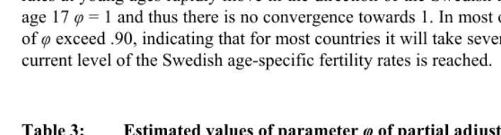
2008 by OLS using equation (13). Table 3 shows the estimated values of φ. For ages 34
and 40 the values of φ are below 1 for all countries. This indicates that there is a clear
tendency towards the Swedish levels of fertility rates for women in their 30s. For
Poland ages 21 and 25 have relatively low values of φ. This indicates that the fertility
rates at young ages rapidly move in the direction of the Swedish levels. In contrast, for
age 17 φ = 1 and thus there is no convergence towards 1. In most other countries values
of φ exceed .90, indicating that for most countries it will take several decades before the
current level of the Swedish age-specific fertility rates is reached.
Table 3: Estimated values of parameter φ of partial adjustment model
age 17 age 21 age 25 age 29 age 34 age 40
Denmark 0.67 0.82 0.89 0.92 0.92 0.94
France 1.00 0.99 0.99 0.89 0.95 0.94
Germany 0.99 0.93 0.95 1.00 0.97 0.97
Italy 0.89 1.00 1.00 1.00 0.96 0.94
Poland 1.00 0.84 0.75 0.96 0.98 0.99
United Kingdom 0.98 0.97 0.82 0.97 0.96 0.94
Using the estimated values of φ, equation (14) is used to make projections of the
ratios of women in their 30s show an increase, but it will take many years before they reach the value of 1. For Polish women at age 29 the increase towards 1 is more rapid.
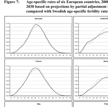
The rate ratios for the year 2030 are used to make projections of the age-specific rates for the six countries. Figure 7 shows that for the three low-fertility countries an increase of fertility rates in women in their late 20s and 30s is projected. Figure 7 shows that the projected age pattern for Denmark is less peaked than the observed pattern in 2008. This can be explained by the fact that the current age pattern for Sweden is less peaked than the Danish pattern. If this is considered implausible, one alternative would be to use the age pattern of another country as the standard age schedule: so, for example, the age pattern of fertility in the Netherlands is more peaked than that in other European countries. Below we will show an alternative scenario. Furthermore Figure 7 shows that the projected age patterns are not smooth for all countries, particularly at young ages for the United Kingdom and Poland, and around the peak age for Germany. The reason why the curve for the United Kingdom is not very smooth is that the age pattern of fertility there at young ages differs strongly from that in Sweden. As a consequence the rate ratios do not show a linear pattern at young ages and thus a linear spline does not produce a very accurate fit. An accurate fit would require additional knots, closer to each other. For Germany the reason why the projected age pattern is not smooth around age 29 is that the projections of the rate ratios for knots next to each
other differ strongly. Table 3 shows that the values of φ differ between ages 25, 29, and
34. If we were to replace the value of φ for age 29 by a value somewhere between the
values for ages 25 and 34, this would produce a smooth age pattern. For the Polish
fertility rates at young ages the same explanation applies: the values of φ for ages 17
Figure 7: Age-specific rates of six European countries, 2008, and scenario for 2030 based on projections by partial adjustment model of rate ratios compared with Swedish age-specific fertility rates
Denmark
0.00 0.02 0.04 0.06 0.08 0.10 0.12 0.14 0.16
15 17 19 21 23 25 27 29 31 33 35 37 39 41 43 45 47 49
United Kingdom
0.00 0.02 0.04 0.06 0.08 0.10 0.12 0.14 0.16
15 17 19 21 23 25 27 29 31 33 35 37 39 41 43 45 47 49
France
0.00 0.02 0.04 0.06 0.08 0.10 0.12 0.14 0.16
15 17 19 21 23 25 27 29 31 33 35 37 39 41 43 45 47 49
Germany
0.00 0.02 0.04 0.06 0.08 0.10 0.12 0.14 0.16
15 17 19 21 23 25 27 29 31 33 35 37 39 41 43 45 47 49
Italy
0.00 0.02 0.04 0.06 0.08 0.10 0.12 0.14 0.16
15 17 19 21 23 25 27 29 31 33 35 37 39 41 43 45 47 49
Poland
0.00 0.02 0.04 0.06 0.08 0.10 0.12 0.14 0.16
15 17 19 21 23 25 27 29 31 33 35 37 39 41 43 45 47 49
Solid line: observed values; dotted line: projections
Table 4 compares the values of the TFR resulting from these projected age-specific fertility rates with the EUROPOP2008 scenario given by Eurostat. Even though, mirroring our assumption, Eurostat assumes convergence towards the Swedish fertility level, our projections of the TFR exceed those of Eurostat. One explanation is that Eurostat assumes a linear change in the direction of the Swedish level, whereas the partial adjustment model that we use implies a non-linear change, as shown by Figure 6. Another important difference between our projections and the Eurostat scenarios is that whereas Eurostat assumes Polish fertility will be lower than that of the other two low-fertility countries, Germany and Italy, our projection for Poland exceeds those for the other two countries. The main explanation is that the projected rate ratio at the peak age (29) increases more strongly for Poland than for Germany and Italy.
Table 4: Total fertility rate (TFR), 2008*, and scenarios for 2030
2008 2030
TOPALS EUROPOP2008
rate ratios compared with
Sweden EU27+3 average
Denmark 1.89 1.90 1.92 1.85
France 2.00 2.01 2.09 1.96
Germany 1.38 1.57 1.55 1.42
Italy 1.37 1.45 1.56 1.46
Poland 1.39 1.62 1.57 1.36
United Kingdom 1.84 1.96 1.94 1.84
* NB. for the United Kingdom TFR in 2006 and for Italy TFR in 2007 instead of 2008.
5.2 Scenarios based on qualitative assumptions
When specifying scenarios of future fertility it is important to identify the main determinants underlying past trends in fertility in order to assess to what extent the trends may be expected to continue. One main trend in fertility across Europe has been the postponement of fertility (Kohler, Billari, and Ortega 2002; Frejka and Sobotka 2008). While northern countries seem to be at the last stage, other countries are at earlier stages (De Beer 2006; Frejka and Sobotka 2008). Billari and Kohler (2004) regard cultural changes (such as secularization and individualism), the rise in the education of women, and the uncertainty during political changes in eastern Europe as the main causes of the postponement. Goldstein (2006) argues that the biological upper age limits of fertility have not yet been reached by far and, consequently, postponement of fertility can continue for decades. Even though to some extent postponement can lead to a decline in the ultimate level of fertility of young cohorts due to the increase of infertility with age, Lanzieri (2009) notes that there is more or less a shared opinion that the catching up of postponed fertility will lead to a rise in the total fertility rate (Bongaarts 2002; Sobotka 2004; De Beer 2006). On the basis of an analysis of recent fertility data Goldstein, Sobotka, and Jasilioniene (2009) conclude that the postponement of fertility “has begun to run its course”. As a consequence they expect a rise of the total fertility rate in the coming decades. Freijka et al. (2008) argue that in the foreseeable future postponement of childbearing to older ages will continue. They assume that in northern and western Europe fertility will be maintained close to the replacement level. In southern, central, and eastern Europe they expect that some increase in fertility rates may occur, but they assume that fertility will remain well below the replacement level. Frejka and Sobotka (2008) mention various explanations of this divide, including cultural differences and differences in family policies.
Figure 8: Linear splines of rate ratios of age-specific fertility rates of six European countries and EU27+3 average, 2008 and 2030
Denmark 0.0 0.2 0.4 0.6 0.8 1.0 1.2 1.4 1.6 1.8
15 17 19 21 23 25 27 29 31 33 35 37 39 41 43 45 47 49 2008 2030 United Kingdom 0.0 0.2 0.4 0.6 0.8 1.0 1.2 1.4 1.6 1.8
15 17 19 21 23 25 27 29 31 33 35 37 39 41 43 45 47 49 2008 2030 France 0.0 0.2 0.4 0.6 0.8 1.0 1.2 1.4 1.6 1.8
15 17 19 21 23 25 27 29 31 33 35 37 39 41 43 45 47 49 2008 2030 Germany 0.0 0.2 0.4 0.6 0.8 1.0 1.2 1.4 1.6 1.8
15 17 19 21 23 25 27 29 31 33 35 37 39 41 43 45 47 49 2008 2030 Italy 0.0 0.2 0.4 0.6 0.8 1.0 1.2 1.4 1.6 1.8
15 17 19 21 23 25 27 29 31 33 35 37 39 41 43 45 47 49 2030 2008 Poland 0.0 0.2 0.4 0.6 0.8 1.0 1.2 1.4 1.6 1.8
15 17 19 21 23 25 27 29 31 33 35 37 39 41 43 45 47 49 2008
Multiplying the assumed values of the rate ratios shown in Figure 8 by the EU27+3 average fertility age schedule produces scenarios of the age-specific fertility rates of the six countries under study. These are shown in Figure 9. Since the scenarios described in Figure 8 show rather smooth age patterns of the rate ratios, the projected age-specific fertility rates shown in Figure 9 are smoother than those shown in Figure 7. One important difference between the scenarios shown in Figure 9 and Figure 7 is that the age patterns for Denmark and France are more peaked in Figure 9. The explanation is that in Figure 8 for these two countries we assume the same values of the rate ratios at age 29 for 2030 as in 2008, whereas the scenarios shown in Figure 7 are based on the less peaked Swedish age pattern. The levels of the TFR implied by these scenarios are shown in Table 4. They are close to the projections based on the assumption of convergence towards the Swedish fertility rates discussed above. The main difference is that the projected level of the TFR for Italy is higher according to the scenario shown in Figure 9. The explanation is that the projections shown in Figure 7 assume no increase
in fertility rates for Italy up to age 29 (since the values of φ equal 1), whereas in Figure
Figure 9: Age-specific rates of six European countries, 2008, and scenario for 2030 based on assumptions on rate ratios compared with
EU27+3 average
Denmark
0.00 0.02 0.04 0.06 0.08 0.10 0.12 0.14 0.16
15 17 19 21 23 25 27 29 31 33 35 37 39 41 43 45 47 49
United Kingdom
0.00 0.02 0.04 0.06 0.08 0.10 0.12 0.14 0.16
15 17 19 21 23 25 27 29 31 33 35 37 39 41 43 45 47 49
France
0.00 0.02 0.04 0.06 0.08 0.10 0.12 0.14 0.16
15 17 19 21 23 25 27 29 31 33 35 37 39 41 43 45 47 49
Germany
0.00 0.02 0.04 0.06 0.08 0.10 0.12 0.14 0.16
15 17 19 21 23 25 27 29 31 33 35 37 39 41 43 45 47 49
Italy
0.00 0.02 0.04 0.06 0.08 0.10 0.12 0.14 0.16
15 17 19 21 23 25 27 29 31 33 35 37 39 41 43 45 47 49
Poland
0.00 0.02 0.04 0.06 0.08 0.10 0.12 0.14 0.16
15 17 19 21 23 25 27 29 31 33 35 37 39 41 43 45 47 49
Solid line: observed values; dotted line: projections
6. Conclusion and discussion
The period TFR is determined not only by changes in the average number of children per woman among successive cohorts, but by changes in the timing of fertility as well. Since the effects of changes in the timing of fertility are temporary, we cannot simply extrapolate from recent changes in the TFR into the future. It is obvious that there are boundaries to changes in fertility rates. One solution is to adjust the level of fertility for changes in the tempo of fertility (see, e.g., Frejka and Sobotka 2008). However, there is some debate about the usefulness of such an adjustment (Van Imhoff 2001; Schoen 2004; Goldstein, Sobotka, and Jasilioniene 2009). An alternative would be to make assumptions about the future values of the age-specific fertility rates rather than about the level of the TFR.
For making projections of future age-specific rates it is useful to use standard age schedules rather than projecting each age-specific fertility rate separately. One approach is to make assumptions about the future values of the parameters of the standard age schedule. A disadvantage of this method is that the values of these parameters tend to be difficult to interpret. Usually they can be interpreted as indicating the direction of changes in the level, timing, and spread of fertility only, but the exact meaning of the value is not clear. Another disadvantage is that “basic” model age schedules do not describe accurately age patterns for all age intervals in all countries at all periods. Consequently several extensions of these models have been proposed in the literature, making them more complicated. A possible way forward is to use splines. They are capable of describing all kinds of age patterns. Splines tend to provide a better fit than parametric models, since parametric models are smoother and thus do not capture deviations in specific age intervals in observed data. However, their usefulness for making projections or creating scenarios is limited, as they do not include interpretable parameters. Another approach is to use relational methods, as proposed by Brass in the 1970s. These models use a standard age schedule, but instead of making assumptions about the future values of the parameters of the age schedule, they make assumptions about the way in which the age pattern to be projected may differ from the standard age schedule. A big advantage of this approach is that the function describing the relationship between the age pattern to be fitted or projected and the standard age schedule is much simpler than the function describing the standard age pattern. One drawback of the Brass method, however, is that it includes two parameters that are difficult to interpret and is therefore not so useful in creating scenarios.
the desired level of goodness of fit and degree of smoothness. In general there is a trade-off: the smoother the age curve, the less accurate the fit. The flexibility of TOPALS implies that the method is less sensitive to the choice of standard age schedule than the Brass model. Therefore one standard curve may be appropriate for describing age-specific fertility rates in countries with different age patterns. However, this does not imply that the choice of the standard age schedule is arbitrary. The more strongly the age pattern of the rates to be fitted differs from the standard age schedule, the more knots are needed to provide an accurate fit. If many knots are needed one may consider choosing another standard age schedule. Visual inspection of the graph of the age pattern of the rate ratios shows immediately whether or not many knots will be needed. If the curve of the rate ratios is significantly non-linear in a particular age interval this implies that many knots will be needed for obtaining a good fit for that age interval. In selecting an appropriate standard age schedule, the main criterion is not the fit with the data but the interpretation of the values of the rate ratios. If the standard age schedule does not have a clear geographical or other relationship with the age-specific rates to be fitted or projected, the values of the rate ratios lack a clear interpretation and thus their usefulness in creating scenarios is limited.
The use of TOPALS for making assumptions about fertility implies that one is making assumptions about the levels of age-specific fertility rates and that the value of the TFR is an outcome, whereas in many countries it is common practice in making projections to first make an assumption about the future values of the TFR and then calculate age-specific rates in line with this assumption. The illustrations in this article show that when using TOPALS to create scenarios one may assume that the changes in fertility rates differ across ages. Rather than assuming only that the total level of fertility will increase or that fertility will be postponed, it is possible to make separate assumptions for different ages. Thus TOPALS makes it possible to create scenarios in which the shape of the age schedule changes. This allows the forecaster to make a distinction between a rise in the mean age at childbearing due to a decrease in fertility rates at very young ages and a rise at older ages caused by the catching up of postponed births. The use of TOPALS makes it possible to estimate whether the fertility age pattern will be more peaked in the future or not. For example, the Netherlands has a relatively high mean age at childbearing but not very high fertility rates at the oldest ages. The reason is that the fertility age pattern in the Netherlands is more peaked than the European average. The Dutch case shows that postponement of fertility will not necessarily result in a postponement of fertility among the oldest ages, which would imply an increase in the number of couples with problems of infecundity. Thus one alternative to the scenarios discussed in the previous section would be to use a combination of Swedish and Dutch fertility rates as standard age schedule: namely, the Dutch age-specific fertility rates multiplied by the ratio of the Swedish and Dutch TFRs. Then one could create a scenario which assumes that other countries will move towards the peaked age pattern of the Netherlands and the relatively high level of Sweden.
TOPALS can be used in combination with other smoothing methods. For example, one may use a cubic spline for producing a smooth age schedule of fertility for a given country in a given year and use TOPALS to make assumptions about future changes in this age schedule. In this case one is trying to explain not the form of the smooth age schedule but rather future changes compared with this standard age schedule. Alternatively TOPALS can be used in combination with a simple parametric model to describe deviations in the age pattern of fertility for a particular country in comparison with this simple model. Applied in this way, TOPALS may be a means of making simple parametric models more complicated. For example, the relatively high fertility rates at young ages in the United Kingdom and Ireland can be described by using the Hadwiger function as standard age schedule, with TOPALS to describe the high fertility rates at young ages.
age-specific fertility rates in other parts of the world as well: for example, using data from the Human Fertility Database (2010), developed by the Max Planck Institute for Demographic Research and the Vienna Institute of Demography. For countries with missing or less reliable or detailed data, TOPALS can be used to estimate single-year age-specific fertility rates: for example, when only data for five-year age groups are available. Brass’s relational model is widely used for this purpose. Using TOPALS, one may choose the age-specific fertility rates of a neighbouring country or a parametric model as the standard age schedule. Furthermore TOPALS may be used for regional population projections. It is common practice to make assumptions about regional differences in fertility rates compared with the national average. Thus one may calculate rate ratios of age-specific fertility rates at regional and at national levels and make assumptions about future changes in these rate ratios.
One of the implications of the flexibility of TOPALS is that it can also be used for describing age-specific rates other than fertility. For example, TOPALS can be used for fitting and projecting age-specific mortality rates (De Beer, Van der Gaag, and Willekens 2007). One final possible application of TOPALS is to create scenarios of age-specific rates taking into account the effects of covariates. For example, when the effect of the level of educational attainment varies between age groups, TOPALS can be used to create scenarios of the rates for different education categories (De Beer, Van der Gaag, and Willekens 2007).