Space-time radial basis function collocation method for one-dimensional
advection-diffusion problem
Marzieh Khaksarfard
Department of Mathematics, Faculty of Mathematical Sciences, Alzahra University, Tehran, Iran.
E-mail: [email protected]
Yadollah Ordokhani
Department of Mathematics, Faculty of Mathematical Sciences, Alzahra University, Tehran, Iran.
E-mail: [email protected]
Mir Sajjad Hashemi∗
Department of Mathematics, Basic Science Faculty, Universiry of Bonab, Bonab, Iran.
E-mail: [email protected]
Kobra Karimi
Department of Mathematics, Buin Zahra Technical University, Buin Zahra, Qazvin, Iran.
E-mail: [email protected]
Abstract The parabolic partial differential equation arises in many application of technolo-gies. In this paper, we propose an approximate method for solution of the heat and advection-diffusion equations using Laguerre-Gaussians radial basis functions (LG-RBFs). The results of numerical experiments are compared with the other ra-dial basis functions and the results of other schemes to confirm the validity of the presented method.
Keywords. Radial basis functions, Heat and advection-diffusion equations, Laguerre-Gaussians functions.
2010 Mathematics Subject Classification. 65M99, 35K20.
1. Introduction
1.1. Introduction of the problem. Parabolic partial differential equations have a wide range of applications for mathematical modelling of many phenomena. There-fore, recently much attention has been paid in the literature to the analysis of accurate methods for the numerical solution of time-dependent partial differential equations. Consider the one-dimensional advection-diffusion equation
ut(x, t) +βux(x, t) =αuxx(x, t), 0< x < L, 0< t≤T, (1.1)
with the initial condition
u(x,0) =f(x), 0≤x≤L, (1.2)
Received: 18 September 2017 ; Accepted: 8 July 2018. ∗Corresponding author.
and the boundary conditions
u(0, t) =g0(t), u(L, t) =g1(t), 0< t≤T, (1.3)
whereβis an arbitrary constant which shows the speed of convection and the diffusion coefficient, i.e. α is a positive constant. We assume that f(x), g0(t) and g1(t) are
suitably given functions. Eq. (1.1) has been used to describe heat transfer in a draining film [25], thermal pollution in river systems [6], the dispersion of dissolved material in estuaries and coastal seas [22], contaminant dispersion in shallow lakes [42], long-range transport of pollutants in the atmosphere [53], water transfer in soils [41], dispersion of dissolved salts in groundwater [19] and flow in porous media [32]. Much efforts has been put into developing accurate numerical methods [28, 29] for the solution of (1.1). Mohebbi [37] proposed a class of new finite difference schemes for solving the one-dimensional heat and advection-diffusion equations. Dehghan [7] presented weighted finite difference techniques for solving this problem. In [48], a high-order compact boundary value method was employed for solution of the heat equations. In the present paper, a numerical scheme will be developed and compared for solving this equation.
1.2. Introduction of the Radial Basis Function. During the recent decades, many numerical methods have been designed for solving various types of problems [1, 2, 21, 23, 24]. Recently, the new advanced computational schemes called meshless methods have been widely employed to solve partial differential equations [4, 5, 49]). The meshless methods based on the radial basis functions are very powerful computa-tional schemes to deal with high-dimensional problems or mathematical models with irregular domain. They are classified into two main categories: strong-form methods such as radial basis collocation schemes (Kansa’s method) [15, 16, 26, 27, 35, 40] and weak-form methods such as radial point interpolation scheme [3, 8, 36, 44-47]. Recently, authors have developed and well-used some meshless methods for solving various types of problems [8-14].
To our best learning, researchers have introduced the space-time meshless formula-tion. Li and Mao published work on the space-time approach using RBFs [34]. They used the global collocation scheme using the Multiquadric function. Netuzhylov de-veloped the space-time meshfree collocation scheme based upon the Interpolating Moving Least Squares (IMLS) method and used it to solve coupled problems with moving boundaries [38]. Young et al. [52] have applied time-dependent fundamental solutions to solve homogeneous diffusion equations. Their proposed method can be considered a space-time collocation scheme as it is free from time discretization.
Some well-known RBFs are listed in Table 1. The kind of RBFs, we will be mostly interested in, are the Gaussiansϕ(r) =e−ε2r2. Other families of radial basis functions
Table 1. Some well-known functions that generate RBFs.
Name of Radial Basis Function Definition Multiquadric(MQ) ϕ(r) =√ε2+r2
Inverse Quadratic(IQ) ϕ(r) = 1 (ε2+r2)
Inverse Multiquadric(IMQ) ϕ(r) =√ 1 ε2+r2
Gaussian(GA) ϕ(r) =e−ε2r2 Thin Plate Splines(TPS) ϕ(r) =r2log(r)
In RBF theory, for a fixed basis function ϕ and shape parameterε, good
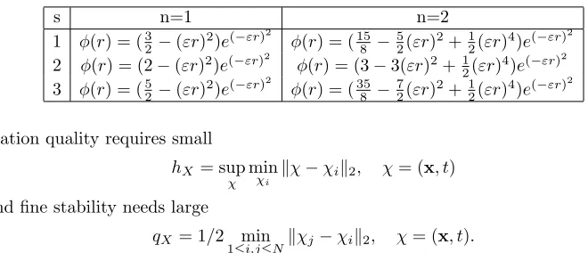
approxi-Table 2. Laguerre-Gaussians radial functions.
s n=1 n=2
1 ϕ(r) = (32−(εr)2)e(−εr)2 ϕ(r) = (15 8 −
5 2(εr)
2+1 2(εr)
4)e(−εr)2
2 ϕ(r) = (2−(εr)2)e(−εr)2 ϕ(r) = (3−3(εr)2+1 2(εr)
4)e(−εr)2
3 ϕ(r) = (5 2−(εr)
2)e(−εr)2
ϕ(r) = (35 8 −
7 2(εr)
2+1 2(εr)
4)e(−εr)2
mation quality requires small
hX= sup χ
min
χi
∥χ−χi∥2, χ= (x, t)
and fine stability needs large
qX= 1/2 min
1≤i,j≤N∥χj−χi∥2, χ= (x, t).
However one cannot minimizehX and maximizeqXat the same time which is referred
to as uncertainty relation in [43]. In the all RBFs consider here, the small shape pa-rameterεdecreases (hX and subsequently) the error of approximation solution and
increases (qX and subsequently) the condition number, and contrariwise. However
many researchers have attempted to develop algorithms for choosing optimal values of the shape parameter but the optimal choice of the shape parameter is still an open question and it is most often selected by brute force. For example, Franke [18] sug-gestedε2 = 1.25D/√N in MQ basis, whereD is the diameter of the smallest circle containing all data points and N is the number of data points. Hardy [20] recom-mended the use ofε2 = 0.815dwhered= (1/N)∑Ni=1di and di is the distance from
the data pointxi to its nearest neighbor. Recently, Fornberg developed a
Contour-Pad´e algorithm that is capable of stably computing the RBF approximation for all ε >0 [17].
2. Radial basis function
2.1. Definition of RBF. LetR+={x∈R, x≥0},∥.∥2denotes the Euclidean norm andϕ:R+ →Rbe a continuous function with ϕ(0)≥0. A radial basis function on
Rd is a function of the form:
which depends only on the distance betweenx∈Rd and a fixed pointxi ∈Rd. So
that the radial basis functionϕiis radially symmetric about the centerxi. Letx1,x2, · · · ,xN ∈Ω⊂Rd be a given set of scattered data. Letr be the Euclidean distance
between a fixed pointxi∈Rd andx∈Rd, i.e. ∥x−xi∥2.
The standard RBFs are categorized into two major classes [14, 31]:
• Class 1. Infinitely smooth RBFs: These basis functions are infinitely differ-entiable and heavily depend on the shape parameterε(such as multiquadric (MQ), Gaussian (GA), inverse multiquadric (IMQ) and inverse quadric (IQ)).
• Class 2. Infinitely smooth (except at centers) RBFs: The basis functions of this category are not infinitely differentiable. These basis functions are shape parameter free and have comparatively less accuracy than the basis functions discussed in Class 1 (such as Thin plate Spline (TPS)).
We have the following theorem about the convergence of RBFs interpolation.
Theorem 2.1. Assume {xi}Ni=1 are N nodes inΩ⊂Rd which is convex, let:
h= max
x∈Ω1≤mini≤N∥x−xi∥2,
whenϕˆ(η)< c(1+|η|)−2l+d, for any y satisfing∫(ˆy(η))2/ϕˆ(η)dη <∞, we have:
∥yN(α)−y(α)∥< chl−α,
whereϕ is RBFs and the constant c depends on the RBFs, ϕˆ andyˆ are supposed to be the Fourier transforms ofϕ andy respectively, y(α) denotes theαth derivative of
y,yN is the RBFs approximation ofy,dis space dimension,l andαare nonnegative integers.
Proof. A complete proof is given by authors [50, 51].
2.2. Function approximation. LetX=L2([0, L]×[0, T]) and
{ϕ00(x, t), ..., ϕ0M(x, t), ϕ10(x, t), ..., ϕ1M(x, t), ..., ϕN0(x, t), ..., ϕN M(x, t)} ⊂X
be the set of RBFs and
H =span{ϕ00(x, t), ..., ϕ0M(x, t), ϕ10(x, t), ..., ϕ1M(x, t), ..., ϕN0(x, t), ..., ϕN M(x, t)},
suppose thathbe an arbitrary element in X. Since H is a finite dimensional vector space,hhas the unique best approximation out of H as hN M ∈H, that is [33]:
∀g∈H,∥h−hN M∥2≤ ∥h−g∥2.
SincehN M ∈H, there exist unique coefficientsc00, ..., c0M, c10, ..., c1M, ..., cN0, ..., cN M
such that:
h≃hN M = N
∑
i=0 M
∑
j=0
cijϕij(x, t) =CTΦN M(x, t) = ΦTN M(x, t)C,
whereC and ΦN M(x, t) are vectors with the form:
C= [c00, ..., c0M, c10, ..., c1M, ..., cN0, ..., cN M]T, (2.1)
3. The solution of the problem via radial basis functions
In This section we present a numerical scheme to solve the one-dimensional advection-diffusion equations using the collocation method and Laguerre-Gaussian radial basis functions. Radial basis function methods are known as a mesh-less scheme for solv-ing partial differential equations numerically. Other methods such as finite-difference methods are known as an efficient class of techniqes for solving PDEs, but there are some problems in using these methods. These schemes are efficient especially for solving problems with arbitrary geometry. But finding a body-fitted mesh is time-consuming and hard to use. Also, it is difficult to obtain results with high order of accuracy.
In the rest of this section we discuss the application of the radial basis functions for solving parabolic partial differential equation.
Let
ut(x, t) +βux(x, t) =αuxx(x, t), (x, t)∈(0, L)×(0, T], (3.1)
with the following initial and boundary conditions:
u(x, t) =f(x), (x, t)∈(0, L)× {0}, (3.2)
u(x, t) =g0(t), (x, t)∈ {0} ×(0, T], (3.3)
u(x, t) =g1(t), (x, t)∈ {L} ×(0, T]. (3.4)
Let
Ξ ={(xi, tj)|xi=L
i
N, tj =T j
M, i= 0,1,· · · , N, j= 0,1,· · ·, M}. (3.5) Using a RBFs method, the solution of the problem is considered as
e u(x, t) =
N
∑
i=0 M
∑
j=0
cijϕij(x, t), (3.6)
wherecij are unknown which remain to be determined andϕij(x, t) is the
Laguerre-Gaussians, i.e. ϕij(x, t) = (2−ε2((x−xi)2+ (t−tj)2))e−ε
2((x−x
i)2+(t−tj)2). Now by the collocation approach we impose the approximate solutionueto satisfy the differ-ential equation and the initial and boundary conditions at (xi, tj), i= 0,1, ..., N, j =
0,1, ..., M. So, we have
e
ut(xi, tj) +βuex(xi, tj) =αuexx(xi, tj), (xi, tj)∈(0, L)×(0, T], (3.7)
e
u(xi, tj) =f(xi), (xi, tj)∈(0, L)× {0}, (3.8)
e
u(xi, tj) =g0(tj), (xi, tj)∈ {0} ×(0, T], (3.9)
e
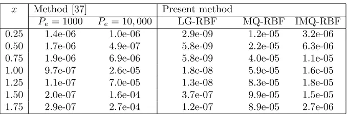
Table 3. Computational results for Example 1.
x Method [37] Present method
Pe= 1000 Pe= 10,000 LG-RBF MQ-RBF IMQ-RBF
0.25 1.4e-06 1.0e-06 2.9e-09 1.2e-05 3.2e-06 0.50 1.7e-06 4.9e-07 5.8e-09 2.2e-05 6.3e-06 0.75 1.9e-06 6.9e-06 5.8e-09 4.0e-05 1.1e-05 1.00 9.7e-07 2.6e-05 1.8e-08 5.9e-05 1.6e-05 1.25 1.1e-07 7.0e-05 1.3e-08 8.3e-05 1.8e-05 1.50 2.0e-07 1.6e-04 3.7e-07 9.9e-05 1.5e-05 1.75 2.9e-07 2.7e-04 1.2e-07 8.9e-05 2.7e-06
which results a linear system of equations. Solving the resulted system, the unknown valuescij, i= 0,1, ..., N, j = 0,1, ..., M can be found. Similarly, we approximate the
solution for MQ and IMQ basis functions.
4. Numerical examples
In this section we give some computational results of numerical experiments with the method based on the preceding sections, to support our theoretical discussion. In the process of computation, all the symbolic and numerical computations are per-formed by using Maple. The readers can see the efficiency of the proposed method from the provided figures and tables in the following examples.
Example 1. Consider Eqs. (1.1)-(1.3) with L = 2, T = 1 and
f(x) = sin(x), g0(t) =e−αtsin(−βt), g1(t) =e−αtsin(1−βt), (4.1)
which has the exact solution
u(x, t) =e−αtsin(x−βt). (4.2)
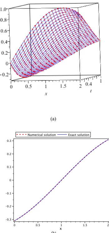
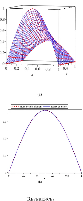
For this problem we putβ = 1. In Table 3 we give the absolute errors with dx = dt= 0.0714 for LG-RBFs withε = 0.5, and for MQ and IMQ basis functions with ε= 5.3 at final timeT = 1. To compare our result we give the absolute errors for the Compact finite difference scheme [37]. Analytical and numerical solutions for 0≤t≤1 andT = 1 are given in Figure 1.
Example 2. Consider the heat equation
ut(x, t) =
1
π2uxx(x, t), (4.3)
withL= 1, T = 1 and
f(x) = sin(πx), g0(t) = 0, g1(t) = 0, (4.4)
which has the exact solution
u(x, t) =e−tsin(πx). (4.5)
Figure 1. Analytical (line) and estimated (point) solutions with dx=dt= 0.0714 andε= 0.5 for (a) 0≤t≤1 and (b) T = 1 from Example 1.
boundary value method [48] and compact finite difference scheme [37]. Analytical and numerical solutions for 0≤t≤1 andT = 1 are given in Figure 2.
5. Conclusion
A RBF-based numerical method was proposed for solving the one-dimensional heat and advection-diffusion equations. The Laguerre-Gaussians radial basis functions (LG-RBFs) on intervalx∈[0, L] andt∈[0, T] were employed. The method was based upon reducing the system into a set of algebraic equations. This algorithm proposed in the current paper was tested for MQ and IMQ functions on several examples from the literature. The obtained results showed that this approach using LG-RBFs can solve the problem effectively.
Acknowledgements
The authors are very grateful to the referees for carefully reading the paper and for their comments and suggestions which have improved the paper.
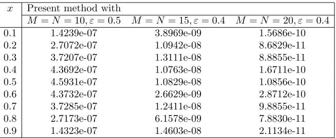
Table 4. Computational results for Example 2.
x Present method with
M =N = 10, ε= 0.5 M =N= 15, ε= 0.4 M =N= 20, ε= 0.4 0.1 1.4239e-07 3.8969e-09 1.5686e-10 0.2 2.7072e-07 1.0942e-08 8.6829e-11 0.3 3.7207e-07 1.3111e-08 8.8855e-11 0.4 4.3692e-07 1.0763e-08 1.6711e-10 0.5 4.5931e-07 1.0829e-08 1.0856e-10 0.6 4.3732e-07 2.6629e-09 2.8712e-10 0.7 3.7285e-07 1.2411e-08 9.8855e-11 0.8 2.7173e-07 6.1578e-09 7.8830e-11 0.9 1.4323e-07 1.4603e-08 2.1134e-11
Table 5. Maximum errors obtained for Example 2.
M =N CBVM [48] method [37] Present method with
Figure 2. Analytical (line) and estimated (point) solutions with dx =dt = 0.1 andε = 0.5 for (a) 0 ≤ t ≤ 1 and (b)T = 1 from Example 2.
References
[2] A. Akg¨ul, Y. Khan, E. K. Akg, D. Baleanu, and M. Al Qurashi,Solutions of Nonlinear Systems by Reproducing Kernel Method, J. Nonlinear Sci. Appl.,10 (2017), 4408–4417.
[3] S. Abbasbandy, H. Roohani Ghehsareh, M. Alhuthali, and H. H. Alsulami, Comparison of meshless local weak and strong forms based on particular solutions for a non-classical 2-D diffusion model, Eng. Anal. Bound. Elem.,39 (2014), 121–128.
[4] M. D. Buhmann,Radial basis functions, Acta. Numer., (2000) 1–38.
[5] M. D. Buhmann,Radial basis functions: theory and implementations, New York: Cambridge University Press, 2004.
[6] M. H. Chaudhry, D. E. Cass, and J. E. Edinger,Modelling of unsteady-flow water temperatures, J. Hydraul. Eng.,109 (1983), 657–669.
[7] M. Dehghan,Weighted finite difference techniques for the one-dimensional advectiondiffusion equation, Appl. Math. Comput.,147 (2004), 307–319.
[8] M. Dehghan and A. Ghesmati,Numerical simulation of two-dimensional sineGordon solitons via a local weak meshless technique based on the radial point interpolation method (RPIM), Comput. Phys. Commun.,181 (2010), 772–786.
[9] M. Dehghan and A. Ghesmati,Combination of meshless local weak and strong (MLWS) forms to solve the two dimensional hyperbolic telegraph equation, Eng. Anal. Bound. Elem.,34 (2010), no. 4, 324–336.
[10] M. Dehghan and V. Mohammadi,The numerical solution of CahnHilliard (CH) equation in one, two and three-dimensions via globally radial basis functions (GRBFs) and RBFs-differential quadrature (RBFs-DQ) methods, Eng. Anal. Bound. Elem.,51 (2015), 74–100.
[11] M. Dehghan and V. Mohammadi,The numerical solution of FokkerPlanck equation with radial basis functions (RBFs) based on the meshless technique of Kansa’s approach and Galerkin method, Eng. Anal. Bound. Elem.,47 (2014), 38–63.
[12] M. Dehghan and A. Nikpour,Numerical solution of the system of second-order boundary value problems using the local radial basis functions based differential quadrature collocation method, Appl. Math. Model.,37 (2013), no. 18, 8578–8599.
[13] M. Dehghan and R. Salahi, A meshfree weak-strong (MWS) form method for the unsteady magnetohydrodynamic (MHD) flow in pipe with arbitrary wall conductivity, Comput. Mech.,
52 (2013), no. 6, 1445–1462.
[14] M. Dehghan and A. Shokri,A meshless method for numerical solution of the onedimensional wave equation with an integral condition using radial basis functions, Numer. Algorithms.,52
(2009), 461–477.
[15] Y. Derel,Solitary wave solutions of the MRLW equation using radial basis functions, Numer. Methods. Partial. Differ. Equ.,28 (2012), 235–247.
[16] Y. Derel, Radial basis functions method for numerical solution of the modified equal width equation, Int. J. Comput. Math.,87(2010), 1569–1577.
[17] B. Fornberg, T. Dirscol, G. Wright, and R. Charles,Observations on the behavior of radial basis function approximations near boundaries, Comput. Math. Appl.,43 (2002), 4730–4490. [18] R. Franke,Scattered data interpolation: tests of some methods, Math. Comp.,38 (1982), 181–
200.
[19] V. Guvanasen and R. E. Volker,Numerical solutions for solute transport in unconfined aquifers, Int. J. Numer. Meth. Fluids.,3 (1983), 103–123.
[20] R. L. Hardy, Multiquadric equations of topography and other irregular surfaces, J. Geophys. Res.,76 (1971), 1905–1915.
[21] M. S. Hashemi, M. Inc, E. Karatas, and A. Akg¨ul,Numerical Investigation on Burgers Equation by MOL-GPS Method, J. Adv. Phys.,6(2017), 413–417.
[22] F. M. Holly and J. M. Usseglio-Polatera,Dispersion simulation in two-dimensional tidal flow, J. Hydraul Eng.,111(1984), 905–926.
[23] M. Inc, B. Kılı¸c, E. Karatas, and A. Akg¨ul, Solitary Wave Solutions for the Sawada-Kotera Equation, Journal of Advanced Physics.,6 (2017), 288–293.
[25] J. Isenberg and C. Gutfinger,Heat transfer to a draining film, Int. J. Heat Transf.,16 (1972), 505–512.
[26] E. J. Kansa, R. C. Aldredge, and L. Ling,Numerical simulation of two-dimensional combustion using mesh-free methods, Eng. Anal. Bound. Elem.,33 (2009), 940–950.
[27] A. G. Kaplan and Y. Derel,Numerical solutions of the symmetric regularized long wave equation using radial basis functions, Comput. Model. Eng. Sci.,84 (2012), 423–438.
[28] H. Karahan, Implicit finite difference techniques for the advection-diffusion equation using spreadsheets, Adv. Eng. Software.,37 (2006), 601–608.
[29] H. Karahan,Unconditional stable explicit finite difference technique for the advection-diffusion equation using spreadsheets, Adv. Eng. Software.,38 (2007), 80–86.
[30] M. Khaksarfard, Y. Ordokhani, and E. Babolian,An efficient approximate method for solution of the heat equation using Laguerre-Gaussians radial functions, Comput. Method. Diff. Eqns.,
4(2016), no. 4, 323–334.
[31] A. J. Khattak, S. I. A. Tirmizi, and S. U. Islam,Application of meshfree collocation method to a class of nonlinear partial differential equations, Eng. Anal. Bound. Elem.,33 (2009), 661–667. [32] N. Kumar, Unsteady flow against dispersion in finite porous media, J. Hydrol., 63 (1988),
345–358.
[33] E. Kreyszig, Introductory Functional Analysis with Applications, John Wiley & Sons Press, New York, 1978.
[34] Z. Li and X. Z. Mao, Global multiquadric collocation method for groundwater contaminant source identification, Environ. Modell. Softw.,26 (2011), 1611–1621.
[35] L. Ling, R. Opfer and R. Schaback, Results on meshless collocation techniques, Eng. Anal. Bound. Elem.,30 (2006), no. 4, 247–253.
[36] G. R. Liu, G. Y. Zhang, Y. T. Gu, and Y. Y. Wang, A meshfree radial point interpolation method (RPIM) for three-dimensional solids, Comput. Mech.,36 (2005), 421–430.
[37] A. Mohebbi and M. Dehghan, High-order compact solution of the one-dimensional heat and advection-diffusion equations, Applied Mathematical Modelling.,34 (2010), 3071–3084. [38] H. Netuzhylov,A space-time meshfree collocation method for coupled problems on
irregularly-shaped domains[Ph.D. thesis]. TU Braunschweig, CSEComputational Sciences in Engineering, 2008.
[39] A. A. Neves, Analysis of laminated and functionally graded plates and shells by a Unified Formulation and Collocation with Radial Basis Functions, A thesis submitted for the Doctoral Degree, 2012.
[40] K. Parand, S. Abbasbandy, S. Kazem, and A. R. Rezaei, Comparison between two common collocation approaches based on radial basis functions for the case of heat transfer equations arising in porous medium, Commun. Nonlinear Sci. Numer. Simul.,16 (2011), 1396–1407. [41] J. Y. Parlarge,Water transport in soils, Ann. Rev. Fluids Mech.,2(1980), 77–102.
[42] J. R. Salmon, J. A. Liggett, and R. H. Gallager,Dispersion analysis in homogeneous lakes, Int. J. Numer. Meth. Eng.,15 (1980), 1627–1642.
[43] R. Schaback, Error estimates and condition numbers for radial basis function interpolation, Adv. Comput. Math.,3(1995), 251–264.
[44] E. Shivanian, Analysis of meshless local radial point interpolation (MLRPI) on a nonlinear partial integro-differential equation arising in population dynamics, Eng. Anal. Bound. Elem.,
37 (2013), 1693–1702.
[45] E. Shivanian,Meshless local Petrov-Galerkin (MLPG) method for threedimensional nonlinear wave equations via moving least squares approximation, Eng. Anal. Bound. Elem.,50 (2015), 249–257.
[46] E. Shivanian,Analysis of meshless local and spectral meshless radial point interpolation (MLRPI and SMRPI) on 3-D nonlinear wave equations, Ocean Eng.,89 (2014), 173–88.
[47] E. Shivanian, A new spectral meshless radial point interpolation (SMRPI) method: a well-behaved alternative to the meshless weak forms, Eng. Anal. Bound. Elem.,54(2015), 1–12. [48] H. Sun and J. Zhang,A high-order compact boundary value method for solving one-dimensional
heat equations, Numer. Methods Partial Differ. Eq.,19 (2003), 846–857.
[50] Z. M. Wu,Radial basis function scattered data interpolation and the meshless method of nu-merical solution of PDEs, Chin. J. Eng. Math.,19 (2002), 1–12.
[51] Z. M. Wu and R. Schaback, Local error estimates for radial basis function interpolation of scattered data, IMA J. Numer. Anal.,13 (1993), 13–27.