Threshold harvesting policy and delayed ratio-dependent functional
response predator-prey model
Razieh Shafeii Lashkarian∗
Department of Basic science, Hashtgerd Branch, Islamic Azad University, Alborz, Iran.
E-mail: [email protected]
Dariush Behmardi Sharifabad
Department of Mathematics, Alzahra university, Tehran, Iran.
E-mail: [email protected]
Abstract This paper deals with a delayed ratio-dependent functional response predator-prey model with a threshold harvesting policy. We study the equilibria of the system be-fore and after the threshold. We show that the threshold harvesting can improve the undesirable behavior such as nonexistence of interior equilibria. The global analysis of the model as well as boundedness and permanence properties are examined too. Then we analyze the effect of time delay on the stabilization of the equilibria, i.e., we study whether time delay could change the stability of a co-existence point from an unstable mood to a stable one. The system undergoes a Hopf bifurcation when it passes a critical time delay. Finally, some numerical simulations are performed to support our analytic results.
Keywords. Predator-prey model, ratio-dependent functional response, threshold harvesting, time delay, Hopf bifurcation.
2010 Mathematics Subject Classification. 37N25, 92D25.
1. Introduction
Mathematical model for predator-prey interaction is studied originally by Lotka [17] and Volterra [22] as
{
˙
x = γx−αxy, ˙
y = βxy−δy, (1.1)
where xand y are the numbers of prey and predator, respectively. In this classical model the positive parametersγ, α, β, andδstand for growth rate of prey, predation rate, conversion rate to change prey biomass into predator reproduction and death rate of predator, respectively.
Received: 29 June 2016 ; Accepted: 5 November 2016.
∗Corresponding author.
More generally the predator-prey model is the following system
{
˙
x = rx(1−xk)−F(x, y), ˙
y = β F(x, y)−δy. (1.2)
The positive parameters r, k, β and δ represent the prey intrinsic growth rate, the environmental carrying capacity, conversion rate to change prey biomass into predator reproduction and predator’s death rate, respectively. The functionF(x, y) describes predation and is called thefunctional response.
Traditionally,F(x, y) is assumed to be a function of the prey population x,that is,F(x, y) =F(x),where F(x) is a Holling type (II) function [18]. It is shown that a predator-prey model with the prey-dependent functional response, may expose the so-calledparadox of enrichmentor thebiological control paradox[10,20,2,9].
The following ratio-dependent functional response predator-prey model has been suggested by Arditi and Ginzburg in [3]
˙
x = rx(1−xk)−abx+yaxy ,
˙ y = y
(
−d+abx+yηax
)
.
(1.3)
Herea >0 andb >0 are predator’s attack rate and handling time, respectively. System (1.3) exposes neither the paradox of enrichment nor the biological control paradox [4,11,12]. One can simplify (1.3), by rescaling
t→rt, x→x/k y→y/abk.
Therefore the ratio-dependent functional response predator-prey model is written as
˙
x = x(1−x)−x+yαxy,
˙
y = −δy+x+yβxy,
(1.4)
whereα=ar, β= brη, δ= dr.
Moreover, in point of view of human needs such as in fishery, forestry and wildlife management, the harvesting of populations is an interesting subject. Constant, linear and quadratic harvesting have been considered so far, for example see, [16,24,25,21, 19].
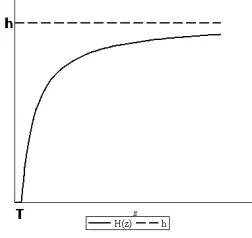
Another harvesting policy is the threshold harvesting. It works as follows: When the population is above of a certain level (threshold) T, the harvesting occurs; when the population falls below that level, the harvesting stops. The policy was first studied by Collie and Spencer [6], and additional analysis has been done since then [1,14,13]. Classically, such harvesting function for a population model is defined as a discontinuous function
ϕ(z) =
{
0 z≤T,
ϵ z > T, (1.5)
Figure 1. Graph of the continuous threshold harvesting function.
z > T. So the continuous threshold function proposed as the following
H(z) =
{
0 z≤T, h(z−T)
h+z−T z > T,
(1.6)
for z = x or z = y [15, 23]. In (1.6), T is the threshold value that determines when harvesting starts or stops and once the population passes T, then harvesting starts and increases smoothly to a limit value h, so the parameter his the rate of harvesting limit. Because of the continuity ofH(z), the managers can adjust the rate of harvesting, more easily, see FIGURE 1.
On the other hand, once the predation occurs, the next generation of predator is not reproduced immediately. So the system (1.4) is impractical in real world.
In this paper we consider a ratio-dependent functional response predator-prey model with a continuous threshold harvesting and with a discrete time delay. In the model, the delay represents the time that takes to predator for consuming prey and to reproduce its next generation. We show that the feedback of the predator density (represented by time delay), might cause the oscillatory behavior.
The subject of this paper is to study the combined effects of harvesting and delay on the dynamics of a ratio-dependent predator-prey model. The reason for choosing this model is that, since we know the dynamics of the system, it will be better for us to determine the effects of delay and harvesting. Furthermore, to the best of our knowledge this is the first time that the global analysis of a delayed ratio-dependent functional response model is studied.
simulations have been done in Section 5, to support the analytic results. Conclusions are made in Section 6.
2. Equilibria of the ratio-dependent functional response model
In this section we consider the following delayed ratio-dependent functional re-sponse predator-prey model with a threshold harvesting policy
˙
x = x(1−x)−x+yαxy,
˙ y = y
(
−δ+x(t−βx(tτ)+y(t−τ)−τ)
)
−H(y),
(2.1)
where
H(y) =
{
0 y≤T, h(y−T)
h+y−T y > T,
(2.2)
and the initial conditions
x0(θ) =ϕ1(θ)≥0, y0(θ) =ϕ2(θ)≥0, θ∈[−τ,0], x(0)>0, y(0)>0,
where (ϕ1, ϕ2)∈C([τ,0],R2+) andxt(θ) =x(t+θ),yt(θ) =y(t+θ).
In this model, the delay represents the time due to converting prey biomass into predator biomass. The functionH(y) is the predator threshold harvesting.
DenoteNx, Ny respectively, the prey and predator nullclines. That is
Nx={(x, y) : x= 0} ∪
{
(x, y) :y= x(x−1) 1−α−x
}
, (2.3)
Ny=
{(x, y) : y= 0} ∪
{
(x, y) :x= βδy−δ
}
y≤T,
{
(x, y) : x= (βδ(h+y−δ)(h+y−T)y−T2+h(y)y−h(y−T)y−T)
}
y > T.
(2.4)
As we are interested in biologically feasible equilibria, we only consider the points in Nx∩Ny∩R2
+, where R2+ is the first quadrant. The system (2.1) has two boundary equilibria O = (0,0), E = (1,0). Furthermore, when y ≤ T, Nx∩Ny has another common elementE∗ = (x∗, y∗) given by
x∗= β−αβ+αδβ ,
y∗= β−δδx∗= x1∗−(xα∗−−x1)∗ =β2−αβ2+2αδββδ −βδ−αδ2. (2.5) Thus the system has an interior equilibriumE∗ in the first quadrant when
β−αβ+αδ >0, β > δ. (2.6)
Note that if 0< α <1, then the conditionβ > δimplies the conditionβ−αβ+αδ > 0.
In the next proposition, we show that fory > T, the system (2.1) has no prey-free equilibrium.
Proposition 2.2. Ify > T, thenNy∩ {(x, y) :x= 0}=∅.
Proof. Assume thaty > T and (x, y)∈Ny∩ {(x, y) :x= 0}. By (2.4) we have
δ(h+y−T)y+h(y−T) = 0. (2.7)
The solutions of (2.7) are
y=−(δh−δT+h)±
√
(δh−δT+h)2+ 4δhT
2δ , (2.8)
and only the following solution is positive
y=−(δh−δT+h) +
√
(δh−δT+h)2+ 4δhT
2δ .
By the following relations it implies thaty < T,a contradiction with the hypothesis.
0>−4δ2T h
⇐⇒(δT +δh+h)2>(δh−δT+h)2+ 4δhT ⇐⇒δT+δh+h >√(δh−δT +h)2+ 4δhT
⇐⇒2δT >−(δh−δT+h) +√(δh−δT +h)2+ 4δhT ⇐⇒T >−(δh−δT+h)+
√
(δh−δT+h)2+4δhT
2δ ⇐⇒T > y.
Thus the system has no prey-free equilibrium in the first quadrant.
By Proposition2.2, ify > T, the interior equilibrium of the system is the solution of the system
y = 1x(x−α−−1)x,
x = (βδ(h+y−δ)(h+y−T)y−2T)y+h(y−h(y−T)y−T).
(2.9)
From the expression y = x(x1−α−−1)x, we know that the points in (2.9) exist in R2 +, if 1−α < x <1. By substituting y = 1x(x−α−−1)x into the expression in Ny, we find that points in (2.9) satisfy the equation
G(x) :=βx5+ (αβ+βT−3β−βh−αδ)x4+ (hα−2βhα+ 2βαT+δhα−δαT+ 3β+ 3βh−3βT +2αδ−2αβ)x3+
(−β−βhα2+ 4βhα−αδ−3βh+ 2δαT−δα2T+βα2T +αβ+hαT+δhα2+ 3βT−2δhα−4βαT−2hα+hα2)x2+ (2βαT−δhα2+hα+δα2T−2βhα−βT−βα2T+δhα +2hα2T−δαT−hα2−2hαT+βh+βhα2)x+
hαT−2hα2T+hα3T = 0.
By the intermediate theoremG(x) has at least one root. Denote byx∗∗, the positive solution of the Eq. (2.10) (if there exists anyone), and let
y∗∗ =x
∗∗(x∗∗−1)
1−α−x∗∗. (2.11)
Ifα≥1 theny∗∗ =x1∗∗−(xα−∗∗x−∗∗1) <1 and we should haveT <1. In this case if
1−T−√(T−1)2−4T(1−α)
2 < x
∗∗< 1−T+ √
(T−1)2−4T(1−α)
2 ,
theny∗∗> T. In the caseα <1 and 1−α−x∗∗≥0, if
x∗∗> 1−T+
√
(T −1)2−4T(1−α)
2 ,
theny∗∗> T. In the caseα <1 and 1−α−x∗∗<0, if
0< x∗∗<1−T+
√
(T−1)2−4(T −T α)
2 ,
theny∗∗> T. Finally if α= 1 and 0< x∗∗<1+√1+4T2 , theny∗∗> T.
The following theorem summarized the above discussions. Note that the theorem, nevertheless, does not reveal under which conditions in harvested model an interior equilibrium appear. We rely on numerical computation to answer this question. In-deed with a numerical simulation in Section 5, we give examples at which the threshold harvesting policy can prevent the extinction of both species, prey and predator. Fur-thermore ifβ > δ andβ−αβ+αδ >0, then the unharvested model has an interior equilibrium (x∗, y∗). Ify∗> T, by the last claim of the theorem the harvested model has an interior equilibrium too.
Theorem 2.3. The boundary equilibria of the system (2.1) in the first quadrant are the co-extinction point O = (0,0) and the predator-free point E = (1,0). If β > δ and β −αβ+αδ > 0, then the unharvested model has a co-existence equilibrium E∗= (x∗, y∗)defined by (2.5). Furthermore if y∗≤T, then E∗ is an equilibrium of the harvested model too. Ify∗> T and(x∗∗, y∗∗)∈R2+, then the harvested model has a co-existence equilibrium E∗∗ = (x∗∗, y∗∗) defined by (2.9) and we have x∗∗ > x∗, T < y∗∗< y∗.
Proof. By the above discussions, we only prove the last claim, which is true by the following lemmas.
Lemma 2.4. Let ˆx= βδy−δ,x˜ = (βδ(h+y−δ)(h+y−T)y−T2+h(y)y−h(y−T)y−T) for a fixed y ≥0. If y > T, thenx >˜ xˆ.
Proof. The following relations prove the result.
0< hy(β−δ)(y−T)⇔
δ(β−δ)(h+y−T)y2−δhy(y−T)< δ(β−δ)(h+y−T)y2+ (β−δ)hy(y−T)⇔
δy β−δ <
δ(h+y−T)y2+h(y−T)y (β−δ)(h+y−T)y−h(y−T) ⇔
Comparing the harvested and unharvested systems, sinceH(y)>0 in [T,+∞) one can easily prove the following lemma.
Lemma 2.5. Lety∗,y∗∗ be the second components of the positive equilibrium of the harvested and unharvested model respectively. Ify∗> T, theny∗∗< y∗.
In other word, while the unharvested coexistence equilibrium is stable, the thresh-old harvesting policy can never increase both populations. In this case coexistence equilibrium have a larger prey population and a lower predator population. With a numerical simulation in Section 5, we give examples at which the threshold harvesting policy can prevent the extinction of both species, prey and predator.
In the rest of this section we study the global qualitative behavior of system (2.1).
Lemma 2.6. The first quadrant is invariant for system (2.1).
Proof. Suppose that there existsA >0, such that for allt∈[0, A), we havex(t)>0, y(t)>0 and eitherx(A) = 0 ory(A) = 0. Consider the following initial value problem
˙
x = x(1−x)−x+˜αx˜yy,
˙˜ y = y˜
(
−δ+x(t−βx(tτ)+˜−y(tτ)−τ)−h+˜yh−T
)
,
˜
y(0) = y(0)>0,
(2.12)
For anyt∈[−τ, A), the following integral equation follows from (2.12)
{
x(t) = x(0) exp∫0t(1−x(s)−x(s)+˜α˜y(s)y(s))ds, ˜
y(t) = y(0) exp∫0t
(
−δ+x(s−βx(sτ)+˜−y(sτ)−τ)−h+˜yh−T
)
ds. (2.13)
From the continuity ofx(t) and ˜y(t) on [−τ, A) one can find a positive number M, such that for allt∈[τ, A),
{
x(t) = x(0) exp∫0t(1−x(s)−x(s)+˜α˜y(s)y(s))ds≥x(0)e−T M, ˜
y(t) = y(0) exp∫0t
(
−δ+x(s−βx(sτ)+˜−y(sτ)−τ)−h+˜yh−T
)
ds≥y(0)e−T M. (2.14)
By standard comparison principal, we havey(t)≥y(t) for all˜ t∈[0,+∞). So for all t∈[τ, A), we have
{
x(t) = x(0) exp∫0t(1−x(s)−x(s)+y(s)αy(s) )ds≥x(0)e−T M, y(t) ≥ y(0) exp∫0t
(
−δ+x(s−βx(sτ)+˜−y(sτ)−τ)− h h+˜y−T
)
ds≥y(0)e−T M. (2.15)
Lemma 2.7. Let (x(t), y(t))be the solution of (2.1). Ifβ > δ, then
lim sup t→+∞
x(t)≤1,
lim sup t→+∞
y(t)≤(β−δ δ )e
βτ.
Proof. From the first equation of system (2.1), one get that for allt∈[0,∞)
˙
x(t)≤x(t)(1−x(t)).
Consider the following initial value problem
{
˙˜
x(t) = x(t)(1˜ −˜x(t)), ˜
x(0) = x(0)>0. (2.16)
By standard comparison principal, we havex(t)≤x(t) for all˜ t∈[0,+∞). Thus
lim sup t→+∞
x(t)≤lim sup t→+∞
˜ x(t) = 1.
From the second equation, we have
˙
y(t)≤βy(t). (2.17)
Thus
y(t)≤y(0)eβt. Thus fort > τ, integrating (2.17) on [t−τ, t], we obtain
y(t−τ)≥y(t)eβτ.
Note that there existsA >0 such that for allt > A, x(t)<1. Hence fort > A+τ,
˙
y(t)≤y(t)
(
β
1 +ye−βτ −δ
)
−H(y)≤y(t)
(
β
1 +ye−βτ −δ
)
.
A standard comparison argument shows that
lim sup t→+∞
y(t)<
(
β−δ δ
)
eβτ.
Hence ifβ > δ, then the system is bounded.
Lemma 2.8. If β−δ−h+MhM−T >0 andα <1, then the system (2.1) has a positive equilibrium, where
M = max{lim sup t→+∞
x(t),lim sup t→+∞
y(t)}.
Proof. One can show easily that if α <1, then
˙
x > x(1−x−α),
which implies that
lim inf
Therefore for anyν >1, there exists a positive Tν such that fort > Tν, x(t)> 1−να andy(t)< νM. Thus fort > Tν+τ, we have
˙
y(t)≥y(t)
(
β1−να 1−α
ν +νM
−δ− νhM
h+νM−T
)
.
Hence
˙
y(t)> y(t)
(
−δ− νhM
h+νM−T
)
,
which implies that fort > Tν+τ,
y(t−τ)> y(t)e(δ+h+νhMνM−T)τ. Thus fort > Tν+τ
˙
y(t)≥y(t)
(
β1−να 1−α
ν +y(t)e( δ+ νhM
h+νM−T)
−δ− νhM
h+νM−T
)
.
which yields
lim inf t→+∞ y(t)≥
(
β1−α ν δ+h+MhM−T −
1−α ν
)
e(δ+h+νhMνM−T)τ.
Asν→1, we get
lim inf t→+∞ y(t)≥
(
β−δ− hM h+M−T
)
(1−α)
δ+ hM h+M−T
e−(δ+h+hMM−T)τ >0.
Recall that system (2.1) is said to be not persistent, if
min(lim inf
t→+∞ x(t),lim inft→+∞ y(t)) = 0, for some of its positive solutions.
Lemma 2.9. Ifα >1 +δ, then the system (2.1) is not persistent.
Proof. Ifα >1 +δ, then there exists anϵ >0 such that α
1 +ϵ = 1 +δ.
Let x(0)y(0) < ϵ, we claim that for allt >0, x(t)y(t)< ϵ. Otherwise, there existst0>0 such that x(t0)
y(t0) =ϵand fort∈[0, t0),
x(t)
y(t)< ϵ. Then fort∈[0, t0), we have
˙
x(t)≤x(t)
(
1− α 1 +ϵ
)
,
from which we obtain
x(t)≤x(0)e(1−1+αϵ) =x(0)e−δt. Thusx(t)≤x(0)e−δt for allt≥0. That is limt
→+∞ x(t) = 0. Similarly,
˙
y(t)≥ −y(t)
(
δ+ h h+y−T
)
from which we obtain
y(t)≥y(0)e−δt. Thus fort∈[0, t0],
x(t) y(t) ≤
x(0)e(1−1+αϵ)
y(0)e−δt = x(0) y(0) < ϵ.
Hence the system is not persistent ifα >1 +δ.
Theorem 2.10. If α >1 +δ and β < α−αδ1−δ, then there exists a positive solution (x(t), y(t))such thatlimt→+∞(x(t), y(t)) = (0,0).
Proof. Ifα >1 +δ, then limt→+∞ x(t) = 0 and for t≥0, x(t)
y(t) ≤ α 1 +δ−1,
provided that
x(0) y(0) ≤
α 1 +δ−1. Hence fort≥τ,
˙
y(t)≤y(t)
(
β
1 + α1+δ−1−δ −δ
)
,
which implies
lim
t→+∞ y(t) = 0,
ifβ < α−αδ1−δ.
One concludes that under the assumptionα >1+δ, system (2.1) may have positive steady state. This shows that system (2.1) can have both positive steady state and positive solutions that tend to the origin.
3. Stability of the equilibria of the model without time delay
In this section, we study the local behavior of the model around its equilibria. The general Jacobian matrix of system (2.1) without delay around an arbitrary point (x, y) equals
J=
1−2x−(x+y)αy22 −
αx2
(x+y)2
βy2
(x+y)2 −δ+
βx2
(x+y)2−
dH(y) dy
, (3.1)
where
dH(y) dy =
{
0 0< y≤T, h2
(h+y−T)2 y > T.
of stability properties and dynamic around the complicated equilibrium (0,0) for unharvested model is done in [5]. SinceT >0, the results of [5] are valid for harvested model too.
From the expression (3.1) the following result can be proved immediately.
Theorem 3.1. At the point E = (1,0), the trace and determinant of (3.1) are T r(J)(1,0)=−1−δ+β andDet(J)(1,0)=δ−β. Therefore
(1) ifδ−β <0 thenE is a saddle; (2) ifδ−β >0 thenE is a stable node; (3) ifδ−β= 0 thenE remains a stable node.
Now we study the linearized system at the interior equilibriaE∗= (x∗, y∗),E∗∗= (x∗∗, y∗∗).
Theorem 3.2. Let
M = (β−δ)(−αδβ
2+αδ2β+β2δ)
β3 ,
N = −β
2+α(β2−δ2)−βδ(β−δ)
β2 .
Ify∗≤T, then we have
(1) ifM <0, thenE∗ is a saddle;
(2) ifM >0 andN <0, thenE∗ is a stable node or focus; (3) ifM >0 andN >0, thenE∗ is an unstable node or focus.
Proof. The Jacobian matrix of system (2.1) atE∗ is
J=
−β2+α(β2−δ2)
β2 −
αδ2 β2
(β−δ)2
β
δ(δ−β) β
.
The associated characteristic equation is
λ2−N λ+M = 0. Thus the eigenvalues of the Jacobian matrix are
λ1,2=
N±√N2−4M
2 ,
and the result is obtained immediately.
Remark 3.3. By Eq. (2.6), if the interior equilibriumE∗ exists, thenM is positive. Thus the coexistence equilibriumE∗cannot be a saddle when it is biologically feasible.
Note that at the equilibrium (x∗∗, y∗∗) the trace and the determinant of the Jaco-bian matrix equals
T r(J) =C−Bα2 −δ+βAα22 −ϕ,
Det(J) =C(αβ2A
2−ϕ−δ) + 1 αB
2(δ+ϕ),
whereϕ= h2 h−T−x∗∗B
A
Theorem 3.4. By the above mentioned notations we have
(1) ifC−α1B2> αβCA2(ϕ+δ)2 , thenE∗∗ is a saddle point;
(2) ifC−α1B2< βCA2
α2(ϕ+δ) andC−
1 αB
2< δ+ϕ−βA2
α2 , thenE∗∗ is a stable node
or focus;
(3) ifδ+ϕ−βAα22 < C−
1 αB
2< βCA2
α2(ϕ+δ), thenE∗∗ is a unstable node or focus.
4. Stabilization effect of the delay
In this section, we study the effect of time delay on the stability of the co-existence equilibrium of the system. The linearized system at the equilibrium (x0, y0) equals
{
u′(t) = a11u(t) +a12v(t),
v′(t) = a21u(t−τ) +a22v(t−τ)−
(
δ+dH(y)dy
)
v(t), (4.1)
whereu(t) =x(t)−x0, v(t) =y(t)−y0,
a11= 1−2x0− αy 2 0
(x0+y0)2, a12=− αx2
0 (x0+y0)2,
a21= βy2
0 (x0+y0)2
, a22= βx2
0 (x0+y0)2
.
Denote system (4.1) by
˙
X(t) =A0X(t) +A1X(t−τ), (4.2)
where
A0=
[
a11 a12
0 −δ−dH(y)d(y)
]
,
and
A1=
[
0 0 a21 a22
]
,
andX(t) = [x(t), y(t)]t. The characteristic equation of (4.1) is
λ2+Aλ+B+ (Cλ+D)e−λτ = 0, (4.3) where
A=−a11+
(
δ+dH(y) dy
)
, B=−a11
(
δ+dH(y) dy
)
,
C=−a22, D=a11a22−a12a21. Whenτ = 0, Eq. (4.3) becomes
λ2+ (A+C)λ+ (B+D). (4.4) All roots of Eq. (4.4) have negative real parts if and only if
(C2): B+D >0.
Recall that the equilibrium (x0, y0) is called absolutely stable if it is asymp-totically stable for all delaysτ ≥0, and is called conditionally stable if it is asymptotically stable forτin some intervals, but not necessarily for all delays τ≥0.
Lemma 4.1. [7] System (4.2) is absolutely stable if and only if (1) Reλ(A0+A1)<0;
(2) det[iωI−A0−A1e−iωτ]̸= 0for all ω >0.
By the first assumption of above lemma, system (4.2) withτ = 0 is asymp-totically stable, while assumption (2) ensures thatiωis not a root of Eq. (4.3). Thus, roughly speaking, Lemma4.1says that the delayed system (4.2) is ab-solutely stable if and only if the corresponding ODE system is asymptotically stable and the characteristic Eq. (4.3) has no purely imaginary roots. Lemma 4.1will be used to study stability and bifurcation in various delayed systems. The main idea is as follows. If assumption (2) does not hold, that is, if the characteristic Eq. (4.3) has a pair of purely imaginary roots, say ±iω0 then system (4.2) is not absolutely stable but can be conditionally stable. Suppose ω0 is achieved whenτ reaches a valueτ0. When τ < τ0 the real parts of all roots of the characteristic Eq. (4.3) still remain negative and system (4.2) is conditionally stable. Whenτ =τ0, the characteristic Eq. (4.3) has a pair of purely imaginary roots±iω0 and system (4.2) loses its stability. By Rouch´es theorem [8] and continuity, if the transversality condition holds at τ = τ0 then when τ > τ0 the characteristic Eq. (4.3) will have at least one root with positive real part and system (4.2) becomes unstable. Moreover, Hopf bifurcation occurs, that is, a family of periodic solutions bifurcates from the steady state asτ passes through the critical valueτ0.
Letλ=iω, ω >0 be the root of the characteristic equation. Then we have −Cωsinτ ω−Dcosτ ω=−ω2+B, (4.5)
−Cωcosτ ω+Dsinτ ω=Aω. (4.6) From this it follows that
ω4−(C2−A2+ 2B)ω2+B2−D2= 0. (4.7) Eq. (4.7) has two roots
ω±= (C
2−A2+ 2B)±√(C2−A2+ 2B)2−4(B2−D2)
2 .
If
On the other hand if
(C4): B2−D2<0 orC2−A2+ 2B >0 and (C2−A2+ 2B)2= 4(B2−D2), then Eq. (4.7) has a positive rootω+. If
(C5): B2−D2>0,C2−A2+ 2B >0 and (C2−A2+ 2B)2>4(B2−D2), then Eq. (4.7) has two positive root ω±. In both cases the characteristic Eq. (4.3) has purely imaginary roots whenτ takes certain values.
From Eq. (4.5) and (4.6) the corresponding critical time delay is given by
τ±= 1 ω±arccos
{
D(ω2
±−B)−ACω±2
C2ω2
±+D2 }
+2jπ
ω±, j= 0,1,2, . . . . (4.8)
The above analysis can be summarized into following lemma.
Lemma 4.2.
(1) If (C1), (C2) and (C4) hold on and τ =τ+, then Eq. (4.3) has a pair of purely imaginary roots ±iω+.
(2) If (C1), (C2) and (C5) hold on andτ=τ+(τ =τ−resp.), then Eq. (4.3) has a pair of conjugate imaginary roots ±iω+ (±iω− resp.).
Letλ±=α±+iω± be the roots of Eq. (4.3) satisfying
α±(τ±) = 0, ω±(τ±) =ω±.
Differentiating (4.3) with respect toτ and substitutingτ=τ±, one can verify that the following transversality conditions hold
d dτ Re λ
+(τ+)>0, d dτ Re λ
−(τ−)<0.
It follows thatτ±are bifurcation values. Thus we have the following theorem.
Theorem 4.3. Let τ± be defined by (4.8), then we have
(1) If (C1)-(C3) hold, then all roots of Eq. (4.3) have negative real parts for all τ≥0.
(2) If (C1), (C2) and (C4) hold, then for τ ∈[0, τ+) all roots of Eq. (4.3) have negative real parts. When τ =τ+, Eq. (4.3) has a pair of purely imaginary roots±iω+ and whenτ > τ+, then Eq. (4.3) has at least one root with positive real part.
(3) If (C1), (C2) and (C5) hold, then forτ ∈[0, τ+)∪(τ−,+∞)all roots of Eq. (4.3) have negative real parts and when τ ∈[τ+, τ−], Eq. (4.3) has at least one root with positive real part.
5. Numerical simulations
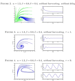
In this section, we present some numerical simulations to illustrate our theoretical analysis. In the first example we show that when the time delay passes the critical time, the system experiences the periodic behavior.
Figure 2. α= 1.3, β= 0.8, δ= 0.4, without harvesting, without delay.
0 0.5 1 1.5
0 0.2 0.4 0.6 0.8 1 1.2 1.4
0 5 10 15 20
0 0.5 1 1.5 t−time x (prey)
0 5 10 15 20
0.2 0.4 0.6 0.8 1 t−time y (predator)
Figure 3. α= 1.3, β= 0.8, δ= 0.4, without harvesting, τ = 1.
0.2 0.25 0.3 0.35 0.4 0.45 0.5 0.55 0.6 0.65 0.25 0.3 0.35 0.4 0.45 0.5 0.55 0.6 x (preys) y (predators)
0 50 100 150 200 0.32 0.34 0.36 0.38 0.4 t−time x (prey)
0 50 100 150 200 0.32 0.34 0.36 0.38 0.4 t−time y (predator)
Figure 4. α= 1.3, β= 0.8, δ= 0.4, without harvesting, τ = 9.
−0.1 0 0.1 0.2 0.3 0.4 0.5 0.6 0.7 −0.1 0 0.1 0.2 0.3 0.4 0.5 0.6 x (preys) y (predators)
0 50 100 150 200 0 0.2 0.4 0.6 0.8 t−time x (prey)
0 50 100 150 200 0.1 0.2 0.3 0.4 0.5 t−time y (predator)
0.1, C =−0.26, D= 0.078. We have A+C > 0 andB+D > 0 and B2−D2 <0, so the conditions (C1), (C2) and (C4) hold on. Hence Eq. (4.7) has a positive root ω+ = 0.202492344and the critical time delay isτ+ = 1
ω+∗arccos(0.75668594)≃3.5.
In FIGURE 3, the phase portrait of the unharvested system with time delayτ = 1 is shown. In FIGURE 4, the phase portrait of the unharvested system with time delay τ= 9 is shown. Sinceτ+<9the system undergoes the oscillatory behavior.
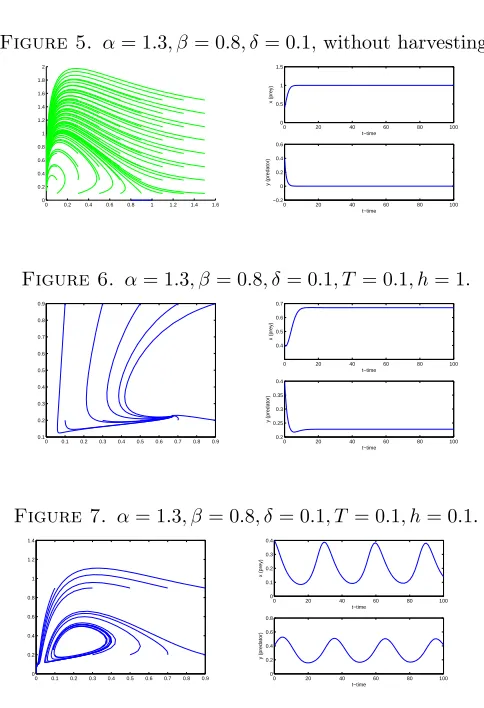
Figure 5. α= 1.3, β= 0.8, δ= 0.1,without harvesting.
0 0.2 0.4 0.6 0.8 1 1.2 1.4 1.6 0 0.2 0.4 0.6 0.8 1 1.2 1.4 1.6 1.8 2
0 20 40 60 80 100 0 0.5 1 1.5 t−time x (prey)
0 20 40 60 80 100 −0.2 0 0.2 0.4 0.6 t−time y (predator)
Figure 6. α= 1.3, β = 0.8, δ= 0.1, T = 0.1, h= 1.
0 0.1 0.2 0.3 0.4 0.5 0.6 0.7 0.8 0.9 0.1 0.2 0.3 0.4 0.5 0.6 0.7 0.8 0.9
0 20 40 60 80 100 0.4 0.5 0.6 0.7 t−time x (prey)
0 20 40 60 80 100 0.2 0.25 0.3 0.35 0.4 t−time y (predator)
Figure 7. α= 1.3, β= 0.8, δ= 0.1, T = 0.1, h= 0.1.
0 0.1 0.2 0.3 0.4 0.5 0.6 0.7 0.8 0.9 0 0.2 0.4 0.6 0.8 1 1.2 1.4
0 20 40 60 80 100 0 0.1 0.2 0.3 0.4 t−time x (prey)
0 20 40 60 80 100 0 0.2 0.4 0.6 0.8 t−time y (predator)
Example 5.2. In FIGURE 5, the phase portrait of the system with the parameter values α= 1.3, β = 0.8, δ= 0.1 without harvesting has been shown. The system has no co-existence equilibria sinceβ−αβ+αδ <0. Then in FIGURE 6, the threshold harvesting function with the parameter valuesh= 1, T = 0.1 is added to the system. In this case, the system has a stable interior equilibrium. Finally in FIGURE 7, the system experience periodic behavior with the harvesting parametersh= 0.1, T = 0.1.
6. Conclusions
equilibria. The system undergoes a Hopf bifurcation when it passes a critical time delay.
7. Acknowledgment
The authors would like to thank the anonymous reviewers for their useful com-ments. The first author would like to acknowledge the funding support of Islamic Azad University, Hashtgerd Branch. This paper is partial result of the project ”On limit cycles of differential equation of damaged DNA by cancer”.
References
[1] S. Aanes, S. Engen, B. Saether, T. Willebrand, and V. Marcstr¨om, Sustainable harvesting
strategies of willow ptarmigan in a fluctuating environment, Ecological Applications, 12(1)
(2002), 281–290.
[2] R. Arditi and A. A. Berryman,The biological control paradox, Trends Ecol. Evol.,6(1)(1991),
32–32.
[3] R. Arditi and L. R. Ginzburg,Coupling in predator-prey dynamics: ratio-dependence, J.
The-oret. Biol.,139(3)(1989), 311–326.
[4] O. Arino, A. El abdllaoui, J. Mikram, and J. Chattopadhyay,Infection in prey population may
act as a biological control in ratio-dependent predator-prey models, Nonlinearity,17(3)(2004), 1101–1116.
[5] F. Berezovskaya, G. Karev and R. Arditi,Parametric analysis of the ratio-dependent
predator-prey model, J. Math. Biol.,43(2001), 221-246.
[6] J. S. Collie and P. D. SpencerManagement strategies for fish populations subject to long term
environmental variability and depensatory predation, Technical Report 93-02, Alaska Sea Grant College 1993; 629–650.
[7] R. Datko, A procedure for determination of the exponential stability of certain differential
difference equations, Quart. Appl. Math.,36(1978), 279–292.
[8] J. Dieudonn´e,Foundations of modern analysis, Academic Press, New York, 1960.
[9] R. Fluck,Evaluation of natural enemies for biological control: a behavioral approach, Trends
Ecol. Evol.,5(6)(1990), 196–199.
[10] N. G. Hairston, F. E. Smith, and L. B. Slobodkin,Community structure, population control
and competition, American Naturalist,94(1960), 421–425.
[11] S. B. Hsu, T. W. Hwang, and Y. Kuang, Global analysis of the Michaeli-Menten-type
ratio-dependent predator-prey system, J. Math. Biol.,42(6)(2001), 489–506.
[12] S. B. Hsu, T. W. Hwang, and Y. Kuang, Rich dynamics of a ratio-dependent one prey two
predator model, J. Math. Biol.,43(5)(2001), 377–396.
[13] R. Lande, S. Engen, and B. Saether,Optimal harvesting of fluctuating populations with a risk
of extinction, Am. Nat.,145(5)(1995), 728–745.
[14] R. Lande, B. Saether, and S. Engen, Threshold harvesting for sustainability of fluctuating
resources, Ecology,78(5)(1997), 1341–1350.
[15] B. Leard, C. Lewis, and J. Rebaza Dynamics of ratio-dependent predator-prey models with
nonconstant harvesting, Disc. Cont. Dynam. Syst.,1(2)(2008), 303–315.
[16] P. Lenzini and J. RebazaNonconstant predator harvesting on ratio-dependent predator-prey
models, Applied Mathematical Sciences,4(16)(2010), 791–803.
[17] A. J. Lotka,Elements of physical biologyWaverly Press, Williams & Wilkins Company,
Balti-more, MD, USA, 1925.
[18] A. F. Nindjin, M. A. Aziz Alaoui, and M. Cadivel, Analysis of a predator-prey models with
modified Leslie-Gower and Holling-type II schemes with time delay, Nonlinear Anal. Real World
[19] M. Rayungsari, W. M. Kusumawinahyu, and Marsudi, Dynamical analysis of predator-prey model with ratio-dependent functional response and predator harvesting, Applied Mathematical
Sciences,8(29)(2014), 1401–1410.
[20] M. L. Rosenzweig,Paradox of enrichment: destabilization of exploitation ecosystems in
ecolog-ical time, Science,171(1971), 385–387.
[21] K. A. Saleh,ratio-dependent predator-prey system with quadratic predator harvesting, Asian
Transactions on Basic and Applied Sciences,2(4)(2013), 21–25.
[22] V. Volterra,Variations and fluctuations of the number of individuals in animal species living
together, ICES J. Cons. int. Explor. Mer.,3(1928), 3–51.
[23] D. Xiao, Jennings L.S.,Bifurcations of a ratio-dependent predator-prey system with constant
rate harvesting, J. Appl. Math.,65(3)(2005), 737–753.
[24] M. Xiao and J. Cao, Hopf bifurcation and non-hyperbolic equilibrium in a ratio-dependent
predator-prey model with linear harvesting rate:analysis and computation, Mathematical and
Computer Modelling,50( 2009), 360–379.
[25] R. Yuan R, W. Jiang, and Y. Wang,Saddle-node-Hopf bifurcation in a modified Leslie-Gower