https://doi.org/10.5194/gmd-11-1293-2018 © Author(s) 2018. This work is distributed under the Creative Commons Attribution 4.0 License.
Estimating criteria pollutant emissions using the California Regional
Multisector Air Quality Emissions (CA-REMARQUE) model v1.0
Christina B. Zapata1, Chris Yang2, Sonia Yeh2, Joan Ogden2, and Michael J. Kleeman1
1Department of Civil and Environmental Engineering, University of California – Davis, Davis, California, USA 2Institute of Transportation Studies, University of California – Davis, Davis, California, USA
Correspondence:Michael J. Kleeman ([email protected]) Received: 16 July 2017 – Discussion started: 8 August 2017
Revised: 24 January 2018 – Accepted: 26 January 2018 – Published: 11 April 2018
Abstract. The California Regional Multisector Air Quality Emissions (CA-REMARQUE) model is developed to predict changes to criteria pollutant emissions inventories in Cal-ifornia in response to sophisticated emissions control pro-grams implemented to achieve deep greenhouse gas (GHG) emissions reductions. Two scenarios for the year 2050 act as the starting point for calculations: a business-as-usual (BAU) scenario and an 80 % GHG reduction (GHG-Step) scenario. Each of these scenarios was developed with an energy eco-nomic model to optimize costs across the entire California economy and so they include changes in activity, fuels, and technology across economic sectors. Separate algorithms are developed to estimate emissions of criteria pollutants (or their precursors) that are consistent with the future GHG sce-narios for the following economic sectors: (i) on-road, (ii) rail and off-road, (iii) marine and aviation, (iv) residential and commercial, (v) electricity generation, and (vi) biore-fineries. Properly accounting for new technologies involving electrification, biofuels, and hydrogen plays a central role in these calculations. Critically, criteria pollutant emissions do not decrease uniformly across all sectors of the econ-omy. Emissions of certain criteria pollutants (or their pre-cursors) increase in some sectors as part of the overall opti-mization within each of the scenarios. This produces nonuni-form changes to criteria pollutant emissions in close proxim-ity to heavily populated regions when viewed at 4 km spa-tial resolution with implications for exposure to air pollution for those populations. As a further complication, changing fuels and technology also modify the composition of reac-tive organic gas emissions and the size and composition of particulate matter emissions. This is most notably apparent through a comparison of emissions reductions for different
size fractions of primary particulate matter. Primary PM2.5
emissions decrease by 4 % in the GHG-Step scenario vs. the BAU scenario while corresponding primary PM0.1emissions
decrease by 36 %. Ultrafine particles (PM0.1) are an
emerg-ing pollutant of concern expected to impact public health in future scenarios. The complexity of this situation illustrates the need for realistic treatment of criteria pollutant emissions inventories linked to GHG emissions policies designed for fully developed countries and states with strict existing envi-ronmental regulations.
1 Introduction
Many countries around the world are debating cost-effective candidate strategies to mitigate threats to long-term prosper-ity including climate change and threats to public health. These specific issues are at least partially linked through re-gional air quality. Realistic mitigation plans for greenhouse gas (GHG) emissions (CO2, CH4, N2O, etc.) usually
in-clude measures encouraging reduced energy consumption or changes to energy sources leading to reduced GHG emis-sions. These measures also impact emissions of criteria pol-lutants or their precursors (particulate matter (PM), NOx, SOx, volatile organic compounds (VOCs), NH3, etc.) that
influence regional air quality. Air quality influences pub-lic health through impacts on mortality (primarily related to PM2.5) and morbidity (primarily related to PM2.5and O3).
also usually performed calculations for large geographic ar-eas without resolving details at regional scales appropriate for California (Bollen et al., 2009; Garcia-Menendez et al., 2015; Rafaj et al., 2012; Shindell et al., 2012; van Aardenne et al., 2010; West et al., 2013). These studies represent Cal-ifornia with only a small number of grid cells or they use simplistic representations of California’s energy economy.
More recent studies addressing interactions between cli-mate policies, emissions, and air quality in the US (Ke-shavarzmohammadian et al., 2017; Loughlin et al., 2011; Ran et al., 2015; Rudokas et al., 2015; Trail et al., 2015; Zhang et al., 2016) have allocated future emissions using en-hanced population surrogates (Ran et al., 2015) and federal climate policies (Trail et al., 2015). The current study builds on this previous work to explicitly account for California’s ambitious climate regulations broken down into detailed sec-tors including realistic siting of biofuel facilities. The cur-rent study also considers the effects of regenerative braking and exhaust particulate size and speciation changes from the heavy use of alternative and renewable fuels across multiple economic sectors. These enhancements support the desired level of detailed analysis for the intersection of air, climate, and energy choices in California.
The purpose of this paper is to describe the Cali-fornia Regional Multisector Air Quality Emissions (CA-REMARQUE) model that can translate complex GHG miti-gation scenarios into criteria pollutant emissions inventories with sufficient detail to support fine-scale air quality mod-els and public health analysis. Here we emphasize solutions that optimize statewide total GHG emissions across the entire California economy, with potential trade-offs between differ-ent source types to achieve this objective. The complex opti-mization problem requires an energy economic model and so we focus on scenarios predicted by the CA-TIMES energy economic model as the starting point for the analysis. The detailed algorithms within the CA-REMARQUE model are then developed to translate predicted changes in GHG emis-sions associated with source activity, fuels, and technology into criteria pollutant emissions that are spatially resolved (4 km) for each sector of the California economy. Changing emissions profiles caused by fuel substitutions are also ac-counted for. Final results are compared to an expert-analysis method developed for a previous global analysis to illustrate why the complex methods described in this study are needed when analyzing developed regions like California that have major diversified economies and a long history of environ-mental regulations.
2 Methodology
Energy scenarios are translated to criteria pollutant emissions inventories by the CA-REMARQUE model in a multistep process with unique algorithms developed for each major sector of the economy that emits air pollution precursors. All
calculations start with energy scenarios developed by the en-ergy economic model CA-TIMES. The details needed to pro-duce criteria pollutant emissions inventories are discussed in the following sections.
2.1 CA-TIMES energy model and energy scenarios CA-TIMES (McCollum et al., 2012; Yang et al., 2014, 2015) is a bottom-up energy–economic model originally based on the TIMES (The Integrated MARKAL-EFOM Sys-tem) model (Loulou et al., 2016). CA-TIMES is a cost-minimization optimization model that balances energy sup-ply and demand system-wide from all energy sectors of the economy. Demand includes the transportation, industrial, residential, commercial, and agricultural sectors. Fuel and electricity supply includes electric, biofuel, hydrogen pro-duction plants, and biofuel and petroleum refineries. De-mand was assumed fixed for the scenarios considered (Yang et al., 2014, 2015). CA-TIMES allows imports from out of state, such as oil, natural gas, and electricity. Renewables and biomass are handled separately and modeled explicitly as located in or out of state and imports are determined on a cost basis. CA-TIMES contains capital and operation costs for each technology and diverse fuel and energy carriers, and it calculates GHG emissions for CO2, CH4, and N2O.
Figure 1.Greenhouse gas emissions in California under the BAU and GHG-Step scenarios.
(California Air Resources Board, 2012b, c, d, e, f), Low Car-bon Fuel Standard (LCFS) (California Air Resources Board, 2009c, 2011c), Cap-and-Trade Program (California Air Re-sources Board, 2011d, 2017), and federal and state incentives (tax credits and subsidies). CA-TIMES predicts total annual energy consumption in California for the year 2050 to be 8763 PJ in the BAU scenario and 7679 PJ in the GHG-Step scenario (reference value for 2010 is approximately 7500 PJ) (Yang et al., 2015).
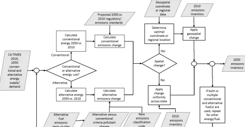
The methods to estimate criteria emissions for different sources developed in the current paper take advantage of the best available information describing future energy and emis-sions as a function of location. The quality of this informa-tion varied considerably for each major source category and so the details of the methodology also varied. Figure 2 illus-trates an overview of the general procedure. The changes in energy consumption and GHG emissions produced by CA-TIMES for each energy sector in the year 2050 were trans-lated into changes in criteria pollutant emissions by account-ing for changaccount-ing energy activity levels or fuel switchaccount-ing. Literature searches were conducted to identify any previ-ous studies describing spatial locations of future emissions within California. Altered emissions for the year 2050 were then projected from a 2010 emissions inventory with 4 km spatial resolution provided by the California Air Resources Board (CARB). Additional details for each major source type are discussed below.
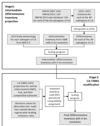
2.2 CA-REMARQUE on-road mobile algorithms On-road mobile sources include passenger cars, light-duty trucks (LDTs), medium-duty trucks (MDTs), heavy-duty trucks (HDTs), buses, motorcycles, and motor homes. On-road emissions were generated in a multistep process sum-marized in Fig. 3. In the first step, 2010–2035 emissions projection trends from the Emission Factor (EMFAC) 2011 model (California Air Resources Board, 2011a) were used
to extrapolate further to 2050. In the second step, an inter-mediate 4 km vehicular emissions inventory was generated by combining EMFAC 2050 projections with a 2010 4 km emissions inventory as a spatial surrogate. In the third step, the 2050 fossil fuel vehicular emissions rates that were pro-jected from EMFAC as well as new emissions rates gathered from alternative fuel emissions literature were used to scale the 4 km intermediate mobile emissions inventory based on the vehicle miles traveled (VMTs), trips, and vehicle class and (conventional and alternative) fuel consumption output produced for each CA-TIMES scenario.
2.2.1 EMFAC emissions and activity projections Criteria pollutant emissions for on-road mobile sources in future years were forecast using the EMFAC 2011 model developed by the California Air Resources Board (CARB) (California Air Resources Board, 2011a). EMFAC 2011 ac-counts for annual VMT trends and vehicle fleet composi-tion turnover using Department of Motor Vehicles (DMV) data. EMFAC incorporates the latest on-road mobile poli-cies including the Low-Emission Vehicle emissions stan-dards, LCFS, Pavley Clean Car Standard, and the Truck and Bus ruling (California Air Resources Board, 2011a). EMFAC 2011 predicts past, present, and future year (up to 2035 or 2040) emissions including anticipated future emissions stan-dards and regulations specific to California. EMFAC predicts emissions and energy activity (VMT, trips, vehicles, gallons of fuel) for 69 geographical area indexes (GAIs) which rep-resent the intersection of air basins and counties (listed in Table S1 in the Supplement).
In the current study, EMFAC was run for each calendar year from 2020 to 2035 to infer the emissions trends that could then be extrapolated to 2050. A simple linear regres-sion model was used to represent VMT over the period 2020– 2035, while a logarithmic regression model was fit to pollu-tant emissions for each vehicle type over the same time pe-riod. Future studies will use EMFAC 2014, which directly predicts emissions in 2050, making this step unnecessary. 2.2.2 Spatial allocation of mobile source emissions in
an intermediate 2050 inventory
An existing on-road mobile emissions inventory for the year 2010 with 4 km spatial resolution served as the starting point for the projection of an intermediate emissions inventory in 2050. Scaling factors to account for VMT growth and adop-tion of existing policies were first calculated as the ratios between EMFAC emissions from 2010 and (extrapolated) 2050 within each of the 69 GAI regions. Separate scaling factors were developed for each pollutant emitted from dif-ferent vehicle classes and control technologies as represented by unique emissions inventory codes (EICs). The combined intermediate emissions (em) scaling factor SFact+met
Figure 2.Process diagram of emissions inventory generation for each sector or mode.
(Eq. 1) and meteorology (met) (Eq. 2). Future 2054 tem-perature and relative humidity generated at 4 km resolution with WRF3.2 (Zhang et al., 2014) were averaged to GAI regions used by EMFAC to produce hour-specific reactive organic gas (ROG) emissions rates that vary from the an-nual average emissions rates. Activity is either defined as VMTs or vehicle trips, depending on the emissions pro-cess. For example, activity equals VMT for tailpipe emis-sions rates (e.g., g NO mile−1) or tire- and brake-wear emis-sions (g PM mile−1). Otherwise, activity equals the number of vehicles within each type, fuel, and aftertreatment cate-gory such as for evaporative emissions of non-methane hy-drocarbons (g NMHC vehicle−1) from the fuel system (non-tailpipe emissions). Emissions rates are highly dependent on the emissions process (evaporative, exhaust, tire or brake wear), fuel (gasoline or diesel), and the aftertreatment device (catalytic or non-catalytic).
Emissions within each 4 km grid cell of the 2010 inventory are multiplied by the 2050 to 2010 scaling factor SFact+metto
estimate the “intermediate” 2050 emissions that will be fur-ther modified according to various additional policy choices represented in CA-TIMES.
SFact=
em(act2050,met2010)
em(act2010,met2010)
(1) SFmet=
em(act2010,met2050)
em(act2010,met2010)
(2)
SFact+met=SFact·SFmet (3)
2.2.3 CA-TIMES modification of intermediate 2050 on-road mobile emissions
Statewide CA-TIMES scaling factors were applied to the 2050 intermediate emissions inventory described in the pre-vious section uniformly at all locations to produce the fi-nal 2050 emissions inventory. EMFAC accounts for popu-lation growth and emissions changes that are required by existing air quality rules and regulations through 2050. CA-TIMES accounts for additional changes that will be required to comply with state GHG targets but which have not yet been placed into emissions rules and regulations. The final inventory retains the spatial and temporal features inherent in the intermediate emissions inventory but incorporates up-dated information about new fuels, technologies, and emis-sions rates based on statewide predictions from CA-TIMES (Fig. 4).
Figure 3.Simplified sequence of algorithms, calculations, and inputs used in developing the CA-TIMES alternative fuel on-road mobile emissions inventory per scenario. EIC is emissions inventory code.
The use of new fuels in the on-road fleet required special consideration during preparation of the 2050 emissions in-ventory. As a starting point, emissions rates from EICs repre-senting conventionally fueled vehicles were calculated from 2050 EMFAC output by dividing each pollutant emissions by the respective vehicle activity indicator (either VMT, ve-hicle number, or fuel consumption) to serve as a baseline for CA-TIMES scenario adjustments. Next, the 181 combi-nations of alternative fuels and electric hybrid, dedicated or single/multi-fueled applications, and vehicle weight classes were mapped to EMFAC by vehicle class and reference fuel (see Tables S2 and S3 in the Supplement). CA-TIMES pre-dicts the amount of alternative fuel consumed, not the VMT associated with that alternative fuel. The VMT associated with each alternative fuel was therefore estimated as the
VMT associated with the conventional fuel divided by the energy content of the consumed conventional fuel (Ev)
mul-tiplied by the energy content of the alternative fuel (Ev, f)
output by CA-TIMES. This calculation assumes that vehi-cle weight and aerodynamics do not change significantly as alternative fuels are adopted. Finally, the emissions rate for each alternative fuel was estimated based on a literature re-view of emissions factors for conventionally vs. alternatively fueled vehicles. Reference emissions rates (erv, ref) and
alter-native to conventional scaling factors (erv, f/erv, ref) for the
vehicle fuels of interest are listed in Table 1.
Equation (4) illustrates how the total emissions (emv) were
CAR LDT MDT HDT MOT BUS CAR LDT MDT HDT MOT BUS CAR LDT MDT HDT MOT BUS 2010 2050 BAU 2050 GHG-step
Hydrogen 0.0 0.0 0.0 0.0 0.0 0.0 21.9 11.8 0.0 0.0 0.0 0.0 159.4 71.6 0.0 0.0 0.0 0.0 Electricity 0.0 0.0 0.0 0.0 0.0 0.4 0.0 0.0 0.0 0.0 0.0 0.0 108.8 38.2 15.2 0.0 0.0 1.5 Biodiesel 0.0 0.0 0.0 0.0 0.0 0.8 0.0 0.0 0.0 0.0 0.0 12.8 6.9 0.0 0.0 227.8 0.0 19.9 E85 0.0 0.0 0.0 0.0 0.0 0.0 98.3 288.0 0.0 0.0 0.0 0.0 0.0 0.0 0.0 0.0 0.0 0.0 Natural gas 0.0 0.0 0.0 0.0 0.0 21.2 0.0 0.0 254.4 0.0 0.0 52.9 0.0 0.0 94.5 0.0 0.0 0.0 Diesel 1.4 0.3 198.4 291.4 0.0 19.1 0.0 0.0 0.0 564.2 0.0 0.0 0.0 0.0 0.0 142.3 0.0 0.1 Gasoline 835 921 124 1.5 5.2 11.7 574.7 502.3 172.4 18.7 7.2 16.1 4.1 10.0 131.7 0.0 5.4 9.1
0 100 200 300 400 500 600 700 800 900 1000
En
er
gy
co
n
su
m
p
ti
o
n
(
P
J)
Figure 4.CA-TIMES energy consumption by vehicle weight class, fuel, and scenario for on-road sources. Vehicle categories include car, light-duty truck (LDT), medium-duty truck (MDT), heavy-duty truck (HDT), motorcycles (MOT), and bus.
Figure 5.Particle emissions size and composition distribution for catalyst-equipped gasoline vehicles(a)and catalyst-equipped ethanol (E85) vehicles(b).
that vehicle as defined by each CA-TIMES scenario. emv=
n X
f
erv, ref·
erv, f
erv, ref
| {z }
·
Alternative fuel/energy emissions rate
actv· Ev, f
Ev ,
| {z }
Proportion of activity by fuel/energy for vehicle
(4)
where v is vehicle type by weight; f is unconventional or al-ternative fuel type fromf1,f2,f3. . .n; ref is reference
(con-ventional) fuel, typically gasoline or diesel; emvis emissions
(t per day) of ROG, CO, NOx, PM10, and SOx for a given vehicle type; erv, ref is pollutant emissions rate for a
vehi-cle using the reference (conventional) fuel based from EM-FAC (t of pollutant VMT−1or t of pollutant vehicle−1); erv, f
Figure 6. Particle emissions size and composition distribution for diesel vehicles(a), biodiesel vehicles(b), and CNG catalyst-equipped vehicles(c).
Figure 7.Particle emissions size and composition distribution for jet-fueled aircraft(a)and biomass-based kerosene jet-fueled aircraft(b).
fuel based from EMFAC (t of pollutant VMT−1or t of pol-lutant vehicle−1); actvis total vehicular activity (not divided
by fuel) (VMT or vehicles);ev, f is energy consumption for
a given fuel by vehicle given by CA-TIMES scenario (PJ); andev is total energy consumed for vehicle for all fuels by
CA-TIMES scenario (PJ).
Alternative fuels considered by CA-TIMES include 95 % volume blend methanol (M95), 85 % volume blend ethanol (E85), compressed natural gas (CNG), liquid petroleum gas (LPG), biodiesel, compressed or liquid hydrogen, and elec-tric drivetrains. Elecelec-tric vehicles include hybrid, plug-in hy-brid, and plug-in or battery hybrid. CA-TIMES often selected the use of multiple technologies and fuels within the same vehicle weight class (see Tables S4 through Table S12 in the Supplement for complete lists). For example, in the case of a hybrid diesel–electric vehicle which runs on three energy sources, diesel, biodiesel, and electricity (e.g., a biodiesel plug-in hybrid MDT), three sets of emissions rates (one for each fuel) were estimated to replace the single emissions rate for the traditional compression ignition (CI) engine for this vehicle class (diesel MDT).
Only approximately 10 % of the possible vehicle type– fuel–engine combinations considered by CA-TIMES (see
Tables S4 to S12 in the Supplement) were actually used in the 2050 BAU and GHG-Step scenarios as the model was optimized for low-cost and low-carbon solutions. The main alternative liquid or gaseous fuels projected by CA-TIMES were E85, biodiesel, and CNG. CA-TIMES predicted that E85 would displace gasoline while biodiesel and CNG would displace diesel based on the dominant fuel consumed for the same vehicle weight class counterpart. This fuel substitution alters emissions rates for criteria pollutants as shown in Ta-ble 1. For battery electric or fuel cell vehicles, the conven-tional fuel displaced was based on the dominant fuel for that vehicle class, e.g., gasoline for LDVs.
2.2.4 On-road mobile particulate matter and gas speciation and size profile changes
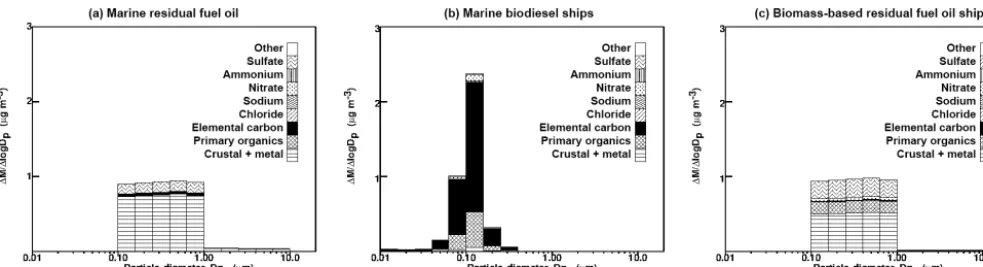
Figure 8. Particle emissions size and composition distribution for ships powered by marine residual oil (a), marine biodiesel (b), and biomass-based residual fuel oil(c).
new VOC and PM emissions profiles (summarized in Ta-bles S14 – S16) for this purpose.
Multiple measurements are available in the literature for the composition of exhaust from ethanol-fueled vehicles. In the present study, the average VOC profiles measured using the Federal Test Procedure, Unified Cycle, and US06 high-speed drive cycles were used for the hot-running E85 VOC exhaust (Haskew and Liberty, 2011). The Federal Test Proce-dure phase 1 profile was applied for the cold-start E85 VOC emissions (Haskew and Liberty, 2011). E85 PM size distribu-tions are summarized in Table S15 in the Supplement (Szy-bist et al., 2011) while PM composition information is sum-marized in Table S16 in the Supplement (Ferreira da Silva et al., 2010; Hays et al., 2013). Figure 5 illustrates the size and composition distribution of PM emitted from catalyst-equipped gasoline vehicles and catalyst-catalyst-equipped vehicles fueled by 85 % ethanol and 15 % gasoline (E85) as an ex-ample.
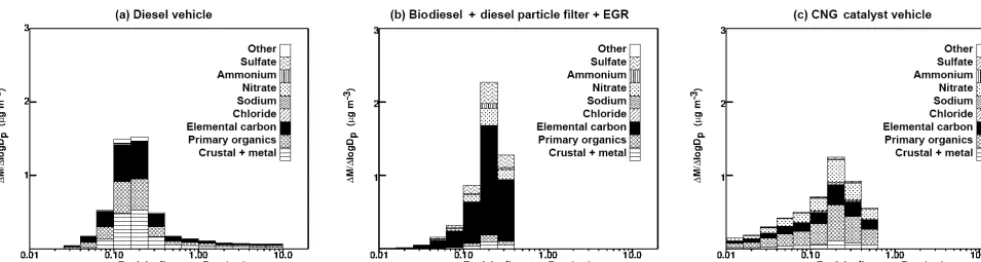
Aftertreatment devices were found to be more influential on biofuel exhaust rates (Alleman et al., 2005; Alleman et al., 2004; Frank et al., 2007; Hasegawa et al., 2007; Rounce et al., 2012; Tsujimura et al., 2007) than changes to fuel prop-erties and feedstock origin (Durbin et al., 2007; Graboski et al., 2003). Diesel particulate filters, exhaust gas recircu-lation, selective catalytic reduction, and oxidation catalyst (OC) were assumed to be deployed on diesel- and biodiesel-powered vehicles by 2050. PM size distributions for vehi-cles equipped with diesel particle filters were obtained from Rounce et al. (2012) (Table S15 in the Supplement), and trace element, carbonaceous, and inorganic ion fractions of PM distributions were obtained from Cheung et al. (2010) and Cheung et al. (2009) (see Table S16 in the Supplement). Gas-phase VOC emissions profiles for biodiesel were not up-dated from fossil diesel profiles in the current study, but this change will be considered in future work.
The CNG VOC profile and PM size distribution was con-structed based on Gautam (2011) (Tables S14 and S15). PM emissions of carbonaceous compounds, metals, and ions were measured from CNG vehicles running on the Urban
Dynamometer Drive Schedules (UDDS) driving cycle (Yoon et al., 2014) (see Table S16 in the Supplement). Figure 6 il-lustrates the size and composition distribution of PM emit-ted from diesel vehicles, biodiesel vehicles equipped with a diesel particle filter and exhaust gas recirculation, and catalyst-equipped CNG vehicles.
All fully electric vehicles, such as battery electric vehicles and H2fuel cell vehicles, were assumed to have zero tailpipe
exhaust and evaporative emissions rates. Brake-wear emis-sions rates were reduced by 59 % (Antanaitis, 2010) for all partial or fully electric vehicles equipped with regenerative breaking, such as hybrid, electric battery, or fuel cell vehi-cles. Tire-wear emissions were assumed to be independent of fuel or technology type.
2.3 CA-REMARQUE aviation, rail, and off-road algorithms
Aviation sources include commercial, civil, agricultural, or military use and primarily run on jet fuel or aviation gaso-line. The rail emissions sources include passenger, com-muter, switching, and hauling trains, which currently run pri-marily on diesel-fueled generators powering an electric driv-etrain. Off-road equipment includes industrial, agricultural, and construction equipment; port and rail operations; and lawn and garden equipment. The list of aviation, rail, and off-road emissions source categorizations are based on the EICs listed in Table S17 in the Supplement (including new EICs created to represent sources operating on alternative fu-els previously not in the CARB inventory).
2.3.1 VISION model
Table 1. Emissions rate changes for alternative fuels in on-road vehicles. Alternative fuels include an 85 % ethanol and 15 % gasoline mixture (E85), biodiesel (B100), and compressed natural gas. Conventional fuels include gasoline, diesel, or ultra-low-sulfur diesel (USLD). Aftertreatment devices include a three-way catalyst (TWC), a diesel oxidation catalyst (DOC), a diesel particle filter (DPF), exhaust gas recirculation ( EGR), and selective catalytic reduction (SCR).
Alternative fuel
Reference conventional
fuel
After-treatment
Pollutant Alt/ conv ratio
Conv % change
Data source
E85 Gasoline Same
(TWC)
CO 1.00 0.0 % Graham et al. (2008)
NOx 0.55 −45 % Graham et al. (2008)
SOx 1.00 0.0 % Assumed
ROG 1.00 0.0 % Graham et al. (2008)
PM 0.25 −75 % Hays et al. (2013)
B100 Diesel or
ULSD
DOC+
DPF+
EGR+
SCR
CO 0.03 −97 % Alleman et al. (2004),
Alleman et al. (2005), Hasegawa et al. (2007)
NOx 0.85 −15 % Alleman et al. (2004), Alleman et al. (2005), Tsujimura et al. (2007)
SOx 1.00 0.0 % Assumed
ROG 0.03 −97 % Alleman et al. (2004), Alleman et al. (2005), Hasegawa et al. (2007)
PM 0.03 −97 % Alleman et al. (2004),
Alleman et al. (2005), Hasegawa et al. (2007), Rounce et al. (2012)
CNG Diesel or
ULSD
TWC CO 0.67 −33 % Cooper et al. (2012)
NOx 0.19 −81 % Cooper et al. (2012)
SOx 1.00 0.0 % Assumed
ROG 0.34 −66 % Cooper et al. (2012)
PM 0.08 −92 % Cooper et al. (2012)
project to the year 2050 while incorporating some future standards for criteria pollutant emissions rates. These include the implementation of Tier 4 130–560 kW compression-ignition diesel engine emissions standards for PM, CO, and NMHC+NOx (California Air Resources Board, 2010a), leading to 90 % reduction in PM emissions rates and an 85 % reduction in NMHC and NOxemissions rates.
Aviation, rail, and off-road 2010 emissions at 4 km reso-lution (em2010cell,I) were scaled to produce an intermediate
esti-mate prior to CA-TIMES adjustments using Eq. (5). em2050cell, i, intermediate= em
2050 i
em2010i
!
·
| {z }
Statewide emissions growth
scaling from 2010 to 2015
em2010cell, i, (5)
em2050i is statewide 2050 emissions of a transport source (kg h−1 or t day−1), em2010
i is statewide 2010 emissions of
a transport source (kg h−1 or t day−1), and em2010 cell, i is grid
cell 2010 emissions of a transport source (kg h−1). 2.3.2 CA-TIMES modification of intermediate 2050
off-road mobile emissions
The portion of energy consumed for each fuel (Ei, f/6fEi, f)
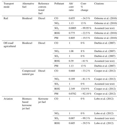
as projected by CA-TIMES was applied to the intermedi-ate 2050 emissions inventory for each transport mode (f) and source type (i) using Eq. (6). The consumption of dif-ferent fuels relative to total fuel consumption for a given mode is shown in Figs. S1–S3 for rail, off-road, and avia-tion modes, respectively. Alternatives to convenavia-tional scaling factors were applied to account for the adoption of alternative fuels as summarized in Table 2. Equation (6) also includes an aftertreatment or control device factor (1−η) where appro-priate.
SFi, f=
Ei, f
P
f Ei, f
·
| {z }
Portion of alternative fuel energy consumption
em2050i, f
em2050 i, intermediate
!
| {z }
Alternative fuel emissions scaling
relative to conventional
· (1−ηi)
| {z }
, Fraction of pollutant not removed by aftertreatment device (6)
where SFi, fis the emissions scaling factor for a given new
or alternative or nonconventional or non-reference fuel for a transport source (dimensionless), Ei, f is new or
alterna-tive fuel or energy consumed by a transport source (e.g., biodiesel for commuter rail) (PJ),P
fEi, fis total fuel or
en-ergy consumed by a transport source (e.g., biodiesel+diesel for commuter rail) (PJ), em2050i, f is statewide 2050 emissions of a transport source consuming a new or alternative fuel (kg h−1 or t day−1), em2050i, intermediate is statewide 2050 inter-mediate emissions of a transport source consuming a new or alternative fuel (kg h−1or t day−1), andηiis efficiency of
re-moval from a control or aftertreatment device (fraction from 0.00 to 1.00).
The final emissions for each specific off-road source con-suming each specific fuel in 2050 (em2050cell, i, f) are then cal-culated by combining the effects of the VISION and CA-TIMES updates as shown in Eq. (7).
em2050cell, i, f=SFi, f·em2050cell, i, intermediate (7)
Aviation biomass-based kerosene jet fuel (KJF) emissions changes are based on Fischer–Tropsch gas-to-liquid biofuel aviation emissions tests (Lobo et al., 2011, 2012). These studies found minor changes to CO and NOxemissions due to the adoption of biofuels. SOxreduction was assumed pro-portional to the fuel sulfur content (Lobo et al., 2012), lead-ing to reductions of 99 % as shown in Table 2.
Off-road equipment (other than trains) operating on biodiesel instead of ultra-low-sulfur diesel (ULSD) was as-sumed to emit HC and NOxwith scaling factors (relative to
conventional diesel emissions) of 0.39 and 1.08, respectively (Durbin et al., 2007). No significant changes in CO, SOxand PM due to the adoption of biodiesel vs. ULSD were identi-fied in the literature and so these emissions were assumed to remain at levels estimated for conventional diesel en-gines. This approach inherently assumes that the sulfur con-tent of biodiesel will not exceed the current limit of 15 ppm for ULSD. Off-road or agricultural emissions changes from switching from diesel to CNG are also found to have large re-ductions in most pollutants except for ROGs (Cooper et al., 2012).
Military aviation emissions were held constant at 2010 levels in the current study due to an assumption of contin-ued exemptions for military activity.
2.3.3 Off-road mobile PM and gas speciation and size profile changes
PM mass size distributions for E85, biodiesel, and CNG are assumed to be similar for off-road and on-road vehicles (Ta-ble S15 in the Supplement). The new PM mass size distribu-tion for biomass-based KJF is shown in Table S18 in the Sup-plement (Lobo et al., 2011). Figure 7 illustrates the size and composition distribution of PM emitted from conventional jet-fuel aircraft and biomass-based KJF aircraft. The conven-tional profile is based on old source profile measurements that assumed uniform distribution of particles between the diameters of 0.1 and 1.0 µm. This conventional profile will be updated with more recent literature values in future work. 2.4 CA-REMARQUE marine algorithms
The marine emissions source category includes all ocean-going vessels (OGVs), commercial harbor craft, and recre-ational boats (see Table S19 in the Supplement). An interme-diate OGV emissions inventory was predicted for the year 2050 based on the extrapolation of Port of Los Angeles and Port of Long Beach 2020 trends (Starcrest Consulting Group, 2009; The Port of Los Angeles and The Port of Long Beach, 2010) (see Table S20 in the Supplement). All other OGV emissions (not listed in Table S20 in the Supplement) in Cal-ifornia were held constant at 2010 levels in the intermediate 2050 inventory prior to modifications from CA-TIMES. 2.4.1 CA-TIMES modification of intermediate 2050
marine emissions
biomass-Table 2.Emissions rate changes for alternative fuels in off-road vehicles.
Transport mode
Alternative fuel
Reference conven-tional fuel
Pollutant Alt/ conv ratio
Conv % change
Citations
Rail Biodiesel Diesel CO 0.655 −34.5 % Osborne et al. (2010)
NOx 1.13 13 % Osborne et al. (2010)
SOx 0.0005 −99.95 % Assumed (see text)
ROG 0.775 −22.5 % Osborne et al. (2010)
PM 0.805 −19.5 % Osborne et al. (2010)
Off-road/ agricultural
Biodiesel Diesel CO 1 0 % Durbin et al. (2007)
NOx 1.08 8 % Durbin et al. (2007)
SOx 1 0 % Durbin et al. (2007)
ROG 0.39 −61 % Assumed (see text)
PM 1.13 13 % Durbin et al. (2007)
Compressed natural gas
Diesel CO 0.668 −33.2 % Cooper et al. (2012)
NOx 0.189 −81.1 % Cooper et al. (2012)
SOx 1 0 % Assumed (see text)
ROG 2.349 134.9 % Cooper et al. (2012)
PM 0.0782 −92.18 % Cooper et al. (2012)
Aviation Biomass-based kerosene jet fuel
Kerosene jet fuel
CO 1 0 % Lobo et al. (2012)
NOx 1 0 % Lobo et al. (2012)
SOx 0.007 −99.3 % Assumed (see text)
ROG 0.605 −39.5 % Lobo et al. (2012)
PM 0.38 −62 % Lobo et al. (2011)
based residual fuel oil (BRFO) in the future, then a third of the RFO marine vessel emissions near California boundaries would also be converted to BRFO. As indicated by Fig. S4 in the Supplement, CA-TIMES finds that other approaches in addition to biofuel adoption for ships are more cost ef-fective for meeting the GHG target in 2050. CA-TIMES de-termined that it will be more economical to substitute some RFO with a lighter petroleum (diesel) to decrease carbon in-tensity rather than using BRFO.
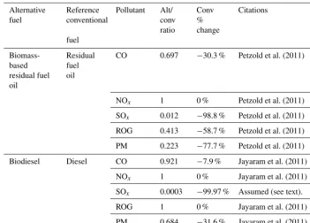
Alternative fuels used in marine sources will modify cri-teria pollutant emissions. Biomass-based alternatives for ma-rine RFO were estimated to be similar to the average of B100 from palm oil, animal fat, soybean oil, and sunflower oil op-erating at 75 % load (Petzold et al., 2011). NOxwas the only
regulated pollutant observed to remain constant during emis-sions testing. Emisemis-sions of all other pollutants decreased as summarized in Table 3.
Assuming biodiesel and BRFO has about 1 ppm of sulfur content, and that by 2010 the sulfur content regulations en-sured that marine diesel oil (MDO) and RFO had 1.5 ppm and 2.5 ppm of S, respectively, then the switch to biofuels would reduce SOxemissions by 33.3 % (relative to conven-tional MDO) and 60 % (relative to convenconven-tional RFO). Ad-ditional reductions in CO, total organic gas (TOG), and PM were also projected based on Jayaram et al. (2011) and Pet-zold et al. (2011) as summarized in Table 3.
summa-Table 3.Emissions rate changes from ships changing from conventional fuels to biofuels.
Alternative fuel
Reference conventional
fuel
Pollutant Alt/ conv ratio
Conv % change
Citations
Biomass-based residual fuel oil
Residual fuel oil
CO 0.697 −30.3 % Petzold et al. (2011)
NOx 1 0 % Petzold et al. (2011)
SOx 0.012 −98.8 % Petzold et al. (2011)
ROG 0.413 −58.7 % Petzold et al. (2011)
PM 0.223 −77.7 % Petzold et al. (2011)
Biodiesel Diesel CO 0.921 −7.9 % Jayaram et al. (2011)
NOx 1 0 % Jayaram et al. (2011)
SOx 0.0003 −99.97 % Assumed (see text).
ROG 1 0 % Jayaram et al. (2011)
PM 0.684 −31.6 % Jayaram et al. (2011)
rized in Tables S21 and S22. At-berth or hotelling container, passenger (cruise), and refrigeration OGVs will use shoreline power instead of auxiliary engines for 80 % of their berthing hours by 2020 (California Air Resources Board, 2007). It was also assumed that MDO or marine gasoline oil used within 24 nautical miles of the California shore will have a sulfur content of<0.1 % by 2050 (California Air Resources Board, 2011e). Further offshore, all marine fuels used within 100 nautical miles of North America were assumed to have a sulfur content<1 % after the year 2012 (leading to the re-ductions shown in Table 3).
2.4.2 Marine PM and gas speciation and size profile changes
PM size distribution changes caused by the switch to alter-native marine fuels were based on Jayaram et al. (2011) (see Table S23 in the Supplement). The size and composition dis-tribution profiles used to represent marine emissions associ-ated with different fuels are displayed in Fig. 8.
2.5 CA-REMARQUE residential and commercial algorithms
Major emissions sources within the residential and com-mercial sectors include natural gas combustion (space heat-ing and water heatheat-ing), biomass combustion (fireplaces and stoves), and food cooking (especially charbroiling and fry-ing). The residential and commercial emissions associated with natural gas and food cooking were assumed to scale according to population growth projected for each county
(Table S24 in the Supplement) (State of California, 2013) to produce an intermediate emissions inventory. These inter-mediate residential and commercial gridded emissions were then scaled to reflect 2010 vs. 2050 results from CA-TIMES (Fig. 9).
Natural gas consumption in the commercial sector was re-duced by half (325 to 162 PJ) in the GHG-Step scenario rela-tive to the BAU scenario in 2050. Most of commercial energy reduction is due to efficiency gains and switch from natu-ral gas to electrification of end uses. Natunatu-ral gas consump-tion in the residential sector also decreases (615 to 507 PJ) under the GHG-Step scenario relative to the BAU scenario. Much of the energy that would have been supplied by natural gas is replaced by renewable sources such as solar (155 PJ), which was assumed to have no criteria pollutant emissions in California. Improved energy efficiency and conservation also plays a role, with residential electricity consumption decreas-ing (402 to 313 PJ) in the GHG-Step scenario. Other combus-tion sources, including wood burning and distillate oil fuel consumption, were allowed to compete in CA-TIMES sub-ject to the constraint that they could not increase above the 2010 levels in order to maintain compliance with current air quality regulations.
2010 2050 BAU 2050
GHG-step 2010 2050 BAU
2050 GHG-step
Commercial Residential
Solar - - 155
Wood 20 -
-Liquid petroleum gas - - - 19 77 76
Natural gas 289 325 162 507 615 224
Electricity 398 361 355 313 402 307
Electricity Electricity Electricity
Electricity Electricity Electricity Natural gas Natural gas
Natural gas
Natural gas
Natural gas
Natural gas Solar
200 400 600 800 1000 1200
En
er
gy
co
n
su
m
p
ti
o
n
(
P
J)
Figure 9.CA-TIMES energy consumption by energy resource and scenario for commercial and residential use.
extracted from national power plant data (US Energy Infor-mation Administration Independent Statistics and Analysis, 2012; US Environmental Protection Agency, 2014). Emis-sions rates per unit of fuel burned were estimated for each power plant described in the base case 2010 emissions in-ventory.
CA-TIMES finds that non-hydro renewable (geother-mal, tidal, solar, wind, and biomass) increases from 10 % (22 938 GWh) of the electricity generation mix in 2010 (144 825 GWh) to 35 and 76 % (489 493 GWh) in the 2050 BAU and 2050 GHG-Step scenarios, respectively (see Fig. 10). However, total in-state and out-of-state electricity generation in the GHG-Step scenario is one-third larger than the BAU scenario (416 219 GWh vs. 643 373 GWh) to meet the increased demand from sectors such as the on-road ve-hicles with growing hybridization and electrification needed to meet the 2050 carbon constraint. Statewide scaling fac-tors for electricity generation in the 2050 BAU scenario vs. 2010 and the 2050 GHG-Step scenario vs. 2010 are listed in Table S25 in the Supplement.
CA-TIMES calculates aggregated statewide energy totals but energy resources (especially for renewables) are not uni-formly distributed across the state. In the current study, re-newable electricity production in 2050 was spatially allo-cated in a manner that was consistent with the energy re-source potential in 12 regions (Fig. S5 in the Supplement) as projected in 15 scenarios by the grid load distribution model SWITCH (Fripp, 2012; Johnston et al., 2013; Nelson et al., 2013). Table S26 in the Supplement lists the electrical
gen-eration by energy source for each SWITCH region averaged across these 15 scenarios. This profile of resource potential was then applied to the CA-TIMES predictions summarized in Table S25 in the Supplement yielding the 2050 and 2010 scaling factors for the BAU scenario (Table S27 in the plement) and the GHG-Step scenario (Table S28 in the Sup-plement).
The scaling factors summarized in Tables S27 and S28 as-sume that the out-of-state portion of electricity generation for a given fuel or energy resource in the year 2050 remained constant at 2010 levels. CA-TIMES does not provide addi-tional information describing out-of-state generation except for a few renewables. This out-of-state portion of the elec-tricity generation was subtracted from the CA-TIMES totals prior to scaling emissions from each power plant in Califor-nia. Table S29 in the Supplement summarizes the out-of-state portion of electricity generation for each fuel in 2010 and as-sumed portions in each of the 2050 scenarios.
Lab-Natural gas
Natural gas
Natural gas Nuclear
Geothermal
Geothermal Hydro
Hydro
Hydro Solar Wind
Wind
Biomass
0.0E+00 1.0E+02 2.0E+02 3.0E+02 4.0E+02 5.0E+02 6.0E+02 7.0E+02
2010 2050 BAU 2050 GHG-step
El
ec
tr
ic
it
y
ge
n
er
at
io
n
(
TW
h
)
Electricity generation
Figure 10.CA-TIMES electricity generation resource mix by scenario.
oratory, 2010). Future biomass IGCC emissions in Califor-nia were estimated using several models that incorporate biomass IGCC, such as GREET, CA-GREET (Argonne Na-tional Laboratory Transportation Technology R&D Center, 2014; California Air Resources Board, 2009a, 2015), and a National Renewable Energy Laboratory analysis (Mann and Spath, 1997). Ultimately, biomass IGCC power plant emis-sions were estimated from conversion of conventional steam turbines in the 2010 CARB inventory based on emissions rates inferred from CA-GREET1.8 for 2050 (Table S33 in the Supplement). An inter-comparison study among GREET1.8, GREET 2014, and GREET2.0 showed that the CA-GREET1.8b model had the best agreement with emissions rates from approximately 30 biomass plants operating on wood residue in California (California Air Resources Board, 2011b; US Environmental Protection Agency, 2014). 2.7 CA-REMARQUE industrial and agricultural
algorithms
The industrial and agricultural emissions category covers many manufacturing industries such as metal, wood, glass, textiles, mining, and chemicals. Food and agricultural sectors
include farming livestock, crops, food production, bakeries, and breweries. Most of these industries were unchanged in the CA-TIMES energy scenarios, with the notable exception that biofuel and hydrogen fuel production replaced some tra-ditional petroleum production, causing changes in refinery and storage emissions (shown in Figs. S6–S8).
2.7.1 Fossil and renewable fuel production
the state rather than extracted locally. This can be seen by the reduction of crude oil supply in California from 1510 PJ in 2010 to 426.5 PJ in the 2050 BAU scenario and 0.0 PJ in the GHG-Step scenario (see Fig. S6 in the Supplement). Re-fining is also projected to decline slightly between the 2010 and 2050 scenarios, with reductions of 25 % in the BAU sce-nario and 44 % in the GHG-Step scesce-nario. This suggests that it is more cost effective or less carbon intensive to import fuel than to extract oil and gas in or around California. The total (imported and in-state) oil supply also decreases in 2050, by −26 % in the BAU (3200 PJ) and−44 % in the GHG-Step scenario (2400 PJ) relative to 2010 (4300 PJ). This reflects the adoption of electrification and alternative fuels to replace petroleum consumption in the presence of growing energy demand in 2050.
Hydrogen (H2) production increased in both 2050
CA-TIMES scenario results, but the increases in the GHG-Step scenario are much larger (Fig. S7 in the Supplement). It was assumed that new hydrogen production facilities would be located at current H2production facilities or existing
re-fineries. Overall 32 new natural gas steam methane reform-ing (SMR) H2facilities and 15 new biomass gasification
fa-cilities were projected to meet the demand summarized in Fig. S7 in the Supplement. In the current study, criteria pollu-tant emissions rates from SMR H2production (summarized
in Table 4) were calculated from the top three SMR H2
pro-duction facilities (California Air Resources Board, 2010c, 2014). Few studies have been published describing crite-ria pollutant emissions from biomass gasification H2
pro-duction and so emissions rates for this propro-duction pathway were obtained from the CA-GREET model (California Air Resources Board, 2015). Direct criteria pollutant emissions from hydrogen production using electrolysis were zero since this process uses electricity to split water molecules into H2
and oxygen (emissions from these facilities appear under electricity generation).
The CA-TIMES model determined that biofuel consump-tion and producconsump-tion will be high in California in the year 2050 (Fig. S8 in the Supplement). Biofuel refineries for dif-ferent feedstock classes (wood, municipal solid waste, herba-ceous crops, yellow grease or tallow, or corn ethanol) (see Tables S34 and S35) were located using a spatial biomass optimization model which seeks to minimize cost within re-source and regulatory constraints (Tittmann et al., 2010). Biofuel refineries were prohibited in NAAQS non-attainment areas, an added constraint based on the high feedstock case described by Parker (2012). Production rates at in-state biore-fineries were scaled to match the in-state volumes produced in CA-TIMES for each type of biofuel. Out-of-state imports and refining were assumed for crops that could not be grown at a large enough scale to meet the demand in California, such as herbaceous crops and the bulk of corn ethanol (see Tables S34 and S35). Emissions for each biofuel refinery were estimated using CA-GREET1.8b emissions rates per unit of fuel produced.
2.7.2 Biogas capture and use
CA-TIMES assumes that landfill gas reduces over time due to better management of organic matter in landfills and the consumption of existing landfill stock material over many decades. All biogas in CA-TIMES is converted to biomethane through removal of CO2and impurities and
fur-ther blended with natural gas so that it is undistinguishable from extracted fossil natural gas.
Dairy biogas is a significant renewable energy source in CA-TIMES. California produced a fifth of the milk in the US in 2010 (California Department of Food and Agricul-ture, 2011) and an exponential regression using 2001–2013 CFDA data estimates the number of dairy cows in Cali-fornia may increase by a factor of 1.5 by the year 2050. Methane emissions rates were estimated from GHG inven-tory documentation (California Air Resources Board, 2014) for each manure management practice: liquid/slurry, anaer-obic lagoon, anaeranaer-obic digester, daily spread, deep pit, pas-ture, and solid storage. The increase in the cow population was assumed to occur uniformly across all management prac-tices except for the systems used in biogas capture. These systems, including anaerobic digester, anaerobic lagoon, and liquid/slurry management practices, were adjusted to meet the quantities of biogas specified by each CA-TIMES sce-nario. The amount of waste produced by each dairy cow each year was used to estimate the annual biomethane production and energy potential of each animal. The electricity poten-tial from biomethane is then calculated using AgSTAR con-version rates (Environmental Protection Agency, 2010; US Environmental Protection Agency AgSTAR Program, 2011). The overall fugitive VOC emissions from animal waste de-clines in the biogas production scenarios since a large frac-tion of the waste is treated. Overall, fugitive dairy manure VOC emissions increased by 50 % due to cow population growth in the BAU scenario and decreased by 33 % for the GHG-Step scenario relative to 2010.
Table 4.Pollutant emissions rate associated with hydrogen production. Units are micrograms of pollutant per kilojoule of hydrogen produced.
SMR – average of Gasification – CA- Electrolysis top CA H2SMR GREET 2015 gasification
facilities vs. SMR scaling
CO 4.079 0.997 0
NOx 1.612 0.34 0
SOx 0.087 0.406 0
VOC 2.208 1.118 0
PM10 0.410 0.048 0
3 Results and discussion 3.1 On-road mobile emissions
Figure 11 illustrates PM emissions of tire and brake wear from on-road vehicles under the BAU and GHG-Step sce-narios. The fine spatial distribution of the emissions reflects the spatial distribution of tire- and brake-wear emissions in the base 2010 inventory that is updated using EMFAC pre-dictions to produce the intermediate 2050 emissions inven-tory. The technology changes inherent in the CA-TIMES BAU and GHG-Step scenarios are then applied uniformly across the state, yielding virtually identical spatial distribu-tions for the final 2050 BAU and GHG-Step scenario emis-sions. Tire- and brake-wear emissions patterns illustrated in Fig. 11 essentially follow predicted vehicle activity patterns in the state. Predicted emissions are highest in major urban centers and along major transportation corridors. Although increase in vehicular activity was part of this study, expan-sion of roadways between 2010 and 2050 was not consid-ered in this study and may be updated in newer versions of the model.
California’s environmental regulations apply uniformly across the state, which supports the assumption of uniform GHG emissions reductions for on-road vehicles. Despite the uniform regulatory landscape, some of the measures de-scribed in the CA-TIMES GHG-Step scenario rely on mod-ified behavioral patterns and willingness or ability to adopt new technologies, which may change by region. Education levels, personal wealth, and environmental attitudes vary sharply across California. Capturing these trends in subre-gions of the state will require surveys of consumer choice and predictions of future behavior that are beyond the scope of the current paper.
Figure 12 illustrates the PM emissions from tailpipe ex-haust under the 2050 BAU scenario and the 2050 GHG-Step scenario. Similar to the tire- and brake-wear emissions, the spatial pattern for mobile sources is identical under both sce-narios because the technology changes specified by the CA-TIMES model are applied uniformly over the entire state. Tailpipe PM emissions once again follow patterns of vehi-cle activity as predicted by EMFAC. Of greater interest is the prediction that tire- and brake-wear emissions (Fig. 11) will
exceed tailpipe emissions (Fig. 12) in both the 2050 BAU and GHG-Step scenarios due to the adoption of increasingly clean vehicle technology. Tailpipe emissions in the GHG-Step scenario are a factor of∼1.8 lower than tailpipe emis-sions in the BAU scenario. In contrast, tire- and brake-wear emissions are predicted to decrease by a factor of+3 under the GHG-Step scenario. This reflects the fact that BAU gaso-line and diesel tailpipe emissions already incorporate signif-icant emissions control technology yielding fewer opportu-nities for further improvement. Tire- and brake-wear emis-sions have almost no control technology in the BAU scenario, which makes the widespread adoption of electric or hybrid drivetrains using regenerative braking particularly effective at reducing emissions.
The current analysis assumes that no new major highways will be built in California and population growth is accom-modated partially through increased urban density such that traffic volumes increase uniformly across the transportation network. These assumptions are simplistic but a previous study of smart growth in the San Joaquin Valley indicated that more detailed accounting of population growth had min-imal impact on air quality (Hixson et al., 2010).
3.2 Rail and off-road emissions
PM emissions from off-road and rail sources are plotted in Fig. 13 for the BAU and GHG-Step scenarios examined in the current study. Maximum statewide PM emissions for this source category are centered at the location of major construction projects with lower emissions rates for “rou-tine” off-road emissions distributed more broadly according to typical activity patterns for smaller construction projects, rail, etc. The 2010 emissions inventory that acts as the ba-sis for the 2050 projections in the current project correctly identified replacement of the east span of the Bay Bridge in the San Francisco Bay Area as the leading construction project with the highest overall emissions in the state. This ∼USD 6.5 billion project spanned more than 10 years, with the new bridge completed in 2013 and final decommissioning and demolition of the old eastern span scheduled for 2018.
Candi-(a) 2050 BAU (μg m min )-2 -1 (b) 2050 GHG-step minus BAU (μg m-2min-1)
Central/ northern CA domain
Southern CA domain
Figure 11.Particulate matter emissions from vehicle tire and break wear in the BAU scenario(a)and emissions change in the GHG-Step scenario(b). Units are µg m−2min−1.
Central/ northern CA domain
Southern CA domain
(a) 2050 BAU (μg m min )-2 -1 (b) 2050 GHG-step minus BAU (μg m-2min-1)
Figure 12.Particulate matter emissions of vehicle tailpipe exhaust in the BAU scenario(a)and emissions change in the GHG-Step scenario (b). Units are µg m−2min−1.
date projects currently under discussion include additional replacement of California’s numerous highways and bridges, upgrading California’s water conveyance systems to better withstand earthquakes, development of high-speed rail lines, reinforcement or expansion of seawalls to protect property, etc. Each of these projects will potentially emit criteria
en-Central/ northern CA domain
Southern CA domain
(a) 2050 BAU (μg m min )-2 -1 (b) 2050 GHG-step minus BAU (μg m-2min-1)
Figure 13.Particulate matter emissions from rail and other off-road sources in the BAU scenario(a)and emissions change in the GHG-Step scenario(b). Units are µg m−2min−1.
sure that the assumed placement of this example major con-struction project does not influence the overall conclusions of the study.
Maximum PM emissions shown in Fig. 13 decrease by a factor of approximately 1.64 in the GHG-Step scenario rel-ative to the BAU scenario. Adoption of biomass-based fuels was also found to reduce emissions of SOx, HC, PM, and oc-casionally CO from off-road and rail sources, but NOx emis-sions increased for some fuel choices.
3.3 Marine and aviation emissions
PM emissions from marine and aviation sources are shown in Fig. 14 for the BAU and GHG-Step scenarios considered in the present study. The highest PM emissions rates occur in offshore shipping lanes that converge on the Port of Los Angeles, the Port of Long Beach, and the Port of Oakland. Emissions rates change with proximity to California shores due to regulations governing sulfur content of marine fuel or ship speed. Emissions patterns at inland locations reflect shipping activity on inland waterways or activity surrounding small regional airports.
Maximum PM emissions rates from marine sources in-crease under the GHG-Step scenario as illustrated most clearly in the right panels of Fig. 14. CA-TIMES determined that the available biofuel capacity could be more efficiently used to offset traditional fossil fuels for on-road transporta-tion sources and so the GHG-Step scenario is predicted to incorporate additional fossil fuels for marine sources under the GHG-Step scenario vs. the BAU scenario. The net re-sult of the disbenefits associated with increased marine
emis-sions vs. the benefits of the decreased on-road emisemis-sions will be considered in future studies that include analysis with re-gional air quality models.
3.4 Residential and commercial emissions
Central/ northern CA domain
Southern CA domain
(a) 2050 BAU (μg m min )-2 -1 (b) 2050 GHG-step minus BAU (μg m-2min-1)
Figure 14.Particulate matter emissions from marine and aviation sources in the BAU scenario(a)and emissions change in the GHG-Step scenario(b). Units are µg m−2min−1.
Central/ northern CA domain
Southern CA domain
(a) 2050 BAU (μg m min )-2 -1 (b) 2050 GHG-step minus BAU (μg m-2min-1)
Figure 15.Particulate matter emissions from residential and commercial sources in the BAU scenario (a)and emissions change in the GHG-Step scenario(b). Units are µg m−2min−1.
3.5 Electricity generation emissions
Figure 16 illustrates predicted emissions of PM from com-bustion processes used to generate electricity. These emis-sions are represented as point sources and so only the grid cells containing an electrical generation unit are colored. The highest emissions rates for individual grid cells are associ-ated with a small number of major electrical generation
Central/ northern CA domain
Southern CA domain
Fi 16 P i l i i f l i i i ( i i 6) i h BAU
(a) 2050 BAU (μg m min )-2 -1 (b) 2050 GHG-step minus BAU (μg m-2min-1)
Figure 16.Particulate matter emissions from electricity generation (emissions source category type 6) in the BAU scenario(a)and emissions change in the GHG-Step scenario(b). Units are µg m−2min−1.
scenario. This fuel switch has a modest impact on total emis-sions given the low utilization of these units.
Peak emissions rates of PM decrease by a factor of∼1.7 in the GHG-Step scenario primarily due to a reduction in fossil fuel electricity generation in favor of a shift to so-lar and wind sources (see Fig. 10). All generating stations are assumed to continue operation at a reduced rate in the GHG-Step scenario rather than selectively decommissioning some stations. The age and efficiency of existing natural-gas-generating stations will likely be key factors determining how they are operated in the future scenarios. Solar and wind electricity generation does not emit criteria pollutants and so the location of these facilities is not shown in Fig. 16. 3.6 Biorefinery emissions
Figure 17 shows the locations of refineries producing bio-fuels (biorefineries) in California under the BAU and GHG-Step scenarios considered in the present study. The location of future biorefineries was chosen to minimize transportation costs for the raw materials feeding into the refinery and the delivery of fuel to the final point of end use. Additional zon-ing constraints were considered to prevent the placement of biorefineries near schools, hospitals, or other locations with sensitive populations. More generally, a constraint was con-sidered to restrict the placement of new biorefineries in re-gions that currently violate the NAAQS. The top panels of Fig. 11 therefore do not allow the placement of biorefineries in either the San Joaquin Valley or the South Coast Air Basin (SoCAB), while the less constrained scenarios illustrated in the lower panels of Fig. 17 do not impose this restriction. In
practice, biorefineries were generally sited near landfills or industrial or agricultural areas within each city selected as economically optimal within the specified constraints. The enforcement of NAAQS constraints on biorefineries led to a smaller number of larger refineries under both the BAU and GHG-Step scenarios. Note that overall biorefining output is higher in the BAU scenario than in the GHG-Step scenario. Biofuels have lower associated GHG emissions than tradi-tional fossil fuels but their carbon intensity is still too high to meet the GHG emissions target represented in the GHG-Step scenario. The CA-TIMES model therefore predicts that a portion of the energy supplied by biofuels in the BAU sce-nario will instead be supplied by wind and solar in the GHG-Step scenario.
3.7 Summary of statewide emissions
(a) BAU scenario (b) GHG-step scenario
With
air q
uali
ty non-attain
ment c
ons
tr
aint
Wi
th
out
ai
r
qu
al
it
y n
on
-a
tt
ai
n
men
t c
ons
trai
n
t (c) (d)
Figure 17.Biorefinery locations under the BAU scenario(a)and the GHG-Step scenario(b). Legend shows PM2.5mass emissions rates per facility (µg m−2min−1). Panels(a)and(b)represent the constrained case in which biorefineries cannot be located in air basins out of compliance with National Ambient Air Quality Standards (NAAQS). Panels(c)and(d)are not constrained by NAAQS status.
in Fig. 18a are not uniform for all pollutants. Maximum re-ductions of ∼60 % are observed for CO2 and particulate
copper (Cu) emissions. In contrast, emissions of particulate SO24−, gaseous CO, and gaseous SOxactually increase under the GHG-Step scenario due to trade-offs in the technologies adopted in the off-road mobile categories (rail, marine, avi-ation, etc.) needed to optimize the overall GHG emissions across the state. Emissions of pollutants that experience creasing trends in Fig. 18a are minor in the present-day in-ventory and so they do not currently trigger NAAQS viola-tions. Changes in key highly emitted pollutants fall in be-tween the extreme cases described above (see results for par-ticulate elemental carbon (EC), parpar-ticulate OC, and gaseous NOx). Each of these pollutants experiences a net decrease in total emissions averaged across California, but emissions changes are not uniform across all categories. Some tech-nology and fuel changes cause higher emissions, which are offset by savings in other categories. This complex mixture of trade-offs reflects the optimal economic approach to GHG reductions determined by the CA-TIMES model.
The changing activity patterns, fuels, and technologies in-cluded in the GHG-Step scenario lead to changes in the emitted particle size and composition distribution. This leads
to differences in the response of primary PM with aerody-namic diameter less than 2.5 µm (PM2.5) and less than 0.1 µm
(PM0.1; ultrafine particles). Ultrafine particles are an
emerg-ing pollutant of concern expected to influence public health (Delfino et al., 2005; Hoek et al., 2010; Knol et al., 2009). The results shown in Fig. 18a illustrate that the GHG-Step scenario leads to only a 4 % decrease in primary PM2.5
emis-sions but a much larger 36 % reduction in PM0.1emissions.
Recent epidemiology results indicate that PM0.1is associated
with mortality in the California Teachers Study (Ostro et al., 2015). Likewise, toxicology studies indicate that ultrafine particles are more toxic than larger particles per unit mass (Donaldson et al., 2001, 2002; Elder et al., 2006; Kreyling et al., 2004; Oberdorster et al., 2002). Enhanced PM0.1
emis-sions reductions could amplify the potential health benefits of the future GHG-Step scenario beyond the level expected from PM2.5emissions reductions.
-80 % -60 % -40 % -20 % 0 % 20 % 40 % 60 % 80 %
Em
is
si
o
n
ra
te
pe
rc
en
t
ch
an
ge
(
%
)
Pollutant
-80 % -60 % -40 % -20 % 0 % 20 % 40 % 60 % 80 %
Em
is
si
o
n
ra
te
pe
rc
en
t
ch
an
ge
(
%
)
Pollutant
Vehicle brake & tire wear
Vehicle exhaust & evaporative Rail & other off-road
Marine & aviation
Residential & commercial Electricity
Industrial & agricultural Miscellaneous
Net total Vehicle brake & tire wear
Vehicle exhaust & evaporative
Rail & other off-road
Marine & aviation
Residential & commercial
Electricity
Industrial & agricultural
Miscellaneous
Net total
(a)
(b)
Figure 18.Change in pollutant emissions rate relative to BAU scenario. Panel(a)represents GHG-Step analyzed in the current study using the CA-TIMES model. Panel(b)represents expert analysis presented by Shindell et al. (2012).
targeted for countries which are in the early stages of adopt-ing policies to reduce GHG emissions or mitigate regional air quality problems. As a result, the measures described by Shindell et al. have a large impact on global public health but they will have a very minor impact on California (or any other major state or country that has already implemented significant emissions controls).
Comparison of Fig. 18a and b illustrates that only re-ductions in particulate EC are comparable in the Shindell et al. and CA-TIMES scenarios due to the mitigation of emis-sions from off-road diesel engines. CA-TIMES accomplishes this reduction through a combined switch in fuels and adop-tion of diesel particle filters on remaining diesel and biodiesel sources to achieve a combined reduction in GHG emissions
and criteria pollutant emissions. Shindell et al. assume uni-form adoption of diesel particle filters on all off-road diesel engines with no fuel switching. Shindell et al. also specify the adoption of digesters for dairy waste and increased use of landfill gas as renewable methane sources. CA-TIMES predicts similar adoption resulting in a∼35–40 % reduction in ammonia (NH3) emissions from these sources. The
Residential and commercial
(a) NOx (ppb ᄹm min )-1 (b) OC (μg m min )-2 -1
Rail and off-road
(c) EC (μg m min )-2 -1 (d) OC (μg m min )-2 -1
Figure 19.Change in emissions in the GHG-Step scenario relative to the BAU scenario.(a)NOxfrom residential and commercial sources (ppb m min−1),(b)particulate OC from residential and commercial sources (µg m−2min−1),(c)particulate EC from off-road and rail sources (µg m−2min−1), and(d)particulate OC from off-road and rail sources (µg m−2min−1).
apparent savings associated with reduced agricultural burns shown in Fig. 18b are likely to have limited practical impact on air quality in the state. Shindell et al. do not consider the adoption of low-carbon fuels or electrification of on-road ve-hicles, which are necessary to achieve deep GHG reductions in CA.
Overall, the analysis presented by Shindell et al. (2012) is appropriately targeted at global health but the measures considered in this analysis do not achieve California’s GHG objectives and the criteria pollutant emissions changes asso-ciated with them will not support calculations for future air quality in California. Energy economic models such as CA-TIMES represent a more realistic tool for development of scenarios in regions like California that have already consid-ered all simple measures. Careful analysis is required to un-derstand the resulting complex pattern of trade-offs between emissions in different categories that result from these sce-narios.
Figure 19 illustrates examples of spatial patterns of emis-sions changes under the GHG-Step scenario predicted by CA-TIMES in the current study. The offsetting increasing and decreasing emissions changes illustrated in Fig. 18 do not occur uniformly over the state but instead appear as re-gions of localized increasing and decreasing emissions. As an even greater complication, the spatial pattern of increas-ing and decreasincreas-ing emissions changes for each pollutant. The top panels of Fig. 19 illustrate changes in the commercial and residential sector for NOxemissions (Fig. 19a) and OC emissions (Fig. 19b) in central California. Patterns of
emis-sions increases or decreases are similar in major urban cen-ters (San Francisco and Sacramento) but different patterns are predicted for emissions of NOx and OC in the heavily polluted San Joaquin Valley (Fresno and Bakersfield). The lower panels of Fig. 19 illustrate even stronger variation in the spatial pattern of emissions changes in the off-road and rail categories in southern California. The spatial pattern of the change in particulate EC emissions (Fig. 19c) differs strongly from the spatial pattern of the change in particulate OC emissions (Fig. 19d).
All of the emissions illustrated in Fig. 19 will produce regions of increased or decreased pollutant concentrations. Given that each region is highly populated, these emissions patterns will have a direct effect on population exposure. Detailed analysis with regional air quality models at a res-olution of 4 km or finer will be required to understand the health implications of these changing emissions. California requires this level of fine-scale emissions analysis to accu-rately predict the air quality impacts of future GHG mitiga-tion strategies in the state. Similar efforts will be required to analyze the effects of GHG mitigation strategies on criteria pollutants in other highly populated regions that have already moved beyond simple emissions regulations banning obvious sources of air pollution.